ANOMALOUS FLUXON PROPERTIES OF LAYERED SUPERCONDUCTORS

1 INTRODUCTION

Highly anisotropic layered superconductors can be considered as stacks of Josephson junctions (SJJ’s) [1, 2]. The key feature of SJJ’s is mutual coupling of junctions, which can be achieved via magnetic [3, 4], charging [5, 6] or non- equilibrium [7] coupling mechanisms. Properties of SJJ’s can be qualitatively different from that of single Josephson junctions (JJ’s) or anisotropic type-II superconductors. This is reflected in a structure of magnetic vortices parallel and perpendicular to superconducting (S) layers. A perpendicular vortex represent an array of 2D pancake vortices in S-layers [8]. Those are Abricosov type vortices with normal cores and with supercurrents flowing in S-layers at a characteristic length $\lambda_{ab}$. Properties of such vortices are well studied, see e.g. Ref. [9], and will not be considered here. For parallel or slightly tilted magnetic field, vortex system commensurates with the layered structure [10] due to intrinsic pinning [11], which tends to locate vortices between S-layers. Such vortices (fluxons) are of Josephson type. They have circulating currents both along and across layers and do not have normal cores.

Fluxon related properties of SJJ’s were extensively studied both analytically and numerically [3,4,12-32], especially in connection with High-$T_{c}$ superconductors (HTSC). Due to a high anisotropy, (weak Josephson coupling between layers), even small in-plane magnetic field causes penetration of fluxons. For Tl and Bi-based HTSC, the penetration field is $\sim$ few Oe [33-35]. Since fluxon energy is low, they can be easily created by thermal excitations [9, 10] or trapped during cooling down. Moreover, because fluxons can not move freely across layers, fluxon-antifluxon pairs in different junctions are stable and can exist even at zero magnetic field [30]. Clearly, a knowledge of fluxon structure is necessary for understanding transport and magnetic properties of layered superconductors. From application point of view, it is particularly interesting to consider SJJ’s with finite number layers, which is the case for HTSC mesas [30,36-43] and low-$T_{c}$ SJJ’s [30,44-54].

Here I will review anomalous single and multi-fluxon properties of SJJ’s. Throughout the paper I will compare analytical, numerical and experimental results both for intrinsic HTSC and artificial low-$T_{c}$ SJJ’s.

2 GENERAL RELATIONS

The most common type of coupling in SJJ’s is magnetic coupling. It appears when S-layers are thinner than London penetration depth, so that magnetic induction is not screened in one junction. SJJ’s are coupled via shared magnetic induction and currents flowing along common electrodes. Properties of magnetically coupled SJJ’s are described by a coupled sine-Gordon equation (CSGE), which was phenomenologically introduced in Ref. [3] and later rigorously derived in Ref. [4]

First, I will briefly describe the formalism of CSGE, following notations of Ref. [20]. Let’s consider a stack of $N$ junctions with the following parameters: $J_{ci}$ -the critical current density, $C_{i}$ and $R_{i}$- the capacitance and the quasiparticle resistance per unit area, respectively, $t_{i}$- the thickness of tunnel barrier, $d_{i}$ and $\lambda_{Si}$ - the thickness and London penetration depth of $S-$layers, respectively, and $L$- the in-plane lengths of the stack. Elements of the stack are numerated from the bottom to the top, so that JJ $i$ consists of S-layers $i$, $i+1$ and a tunnel barrier $i$. The CSGE can be written in a compact matrix form [4]:

$${\bf\varphi}^{\prime\prime}={\bf A\cdot J}_{z}-{\bf J}_{b}$$ (1)

Here ${\bf\varphi}$ is a column of gauge invariant phase differences $\varphi_{i}$, ’primes’ denote in-plane spatial derivatives, ${\bf A}$ is a symmetric tridiagonal $N\times N$ matrix with nonzero elements: $A_{i,i-1}=-S_{i}/\Lambda_{l}$; $A_{i,i}=\Lambda_{i}/\Lambda_{l}$; $A_{i,i+1}=-S_{i+1}/\Lambda_{l}$, where $\Lambda_{i}=t_{i}+\lambda_{Si}coth\left(\frac{d_{i}}{\lambda_{Si}}\right)+\lambda_{Si+1}coth\left(\frac{d_{i+1}}{\lambda_{Si+1}}\right)$, $S_{i}=\lambda_{Si}cosech\left(\frac{d_{i}}{\lambda_{Si}}\right)$. Current density across layers, ${\bf J}_{z}$, consists of supercurrent, displacement current and normal current components:

$$J_{zi}=j_{ci}sin\left(\varphi_{i}\right)+\tilde{C}_{i}\ddot{\varphi}_{i}+\alpha_{i}\dot{\varphi}_{i}.$$ (2)

Here $j_{ci}=\frac{J_{ci}}{J_{cl}}$, $\tilde{C}_{i}=\frac{C_{i}}{C_{l}}$, ’dots’ denote time derivatives, $\alpha_{i}=\sqrt{\frac{\Phi_{0}}{2\pi cJ_{cl}C_{l}R_{i}^{2}}}$ are damping parameters, $\Phi_{0}$ is the flux quantum and $c$ is the velocity of light in vacuum. ${\bf J}_{b}$ is a bias term [20]. Space and time are normalized to Josephson penetration depth, $\lambda_{jl}=\sqrt{\frac{\Phi_{0}c}{8\pi^{2}J_{cl}\Lambda_{l}}}$, and the inverse plasma frequency $1/\omega_{pl}=\sqrt{\frac{\Phi_{0}C_{l}}{2\pi cJ_{cl}}}$ of JJ $l$, respectively.

Magnetic induction in a stack is given by:

$${\bf B}=\frac{H_{0}}{2}{\bf A}^{-1}{\bf\varphi}^{\prime}.$$ (3)

Here $H_{0}=\Phi_{0}/(\pi\lambda_{jl}\Lambda_{l})$.

Table 1: Parameters of LD model in terms of CSGE and estimations for Bi2212 HTSC

LD	$\lambda_{ab}$	$\lambda_{c}=\gamma\lambda_{ab}$	$\lambda_{J}=\gamma s$
CSGE	$\lambda_{s}\sqrt{\frac{s}{d}}$	$\sqrt{\frac{\Phi_{0}c}{8\pi^{2}J_{c}s}}$	$\sqrt{\frac{\Phi_{0}cd}{16\pi^{2}J_{c}\lambda_{s}^{2}}}=\frac{\lambda_{J}(\text{LD})}{\sqrt{2}}$
Bi2212	0.15-0.2 $\mu m$	130-184 $\mu m$	$\lambda_{J}($CSGE$)=$0.6-1.1 $\mu m$

For $d/\lambda_{s}\ll 1$, equations analogous to Eq.(1) were derived from Lawrence-Doniach (LD) [1] model [14, 16]. The LD-CSGE conversion is shown in Table 1, along with estimations for Bi2212 HTSC ($d$=3 Å, $t$ =12 Å, $J_{c}$=500-1000 A/cm², $\lambda_{s}$=750-1000 Å).

In static case, CSGE reduces to

$${\bf\varphi}^{\prime\prime}={\bf A\cdot}j_{c}sin({\bf\varphi}).$$ (4)

For non-dissipative fluxon motion with a velocity $u$, the phase distribution remains unchanged in a coordinate frame moving along with the fluxon, $\xi=x-ut$, and CSGE can be simplified [32]

$${\bf D\cdot\varphi}^{\prime\prime}={\bf A\cdot}j_{c}sin({\bf\varphi}),$$ (5)

where ${\bf D}={\bf E}-u^{2}\tilde{C}{\bf A}$, and ${\bf E}$ is the unitary matrix.

The first integral: CSGE has a first integral [20]

$$\frac{1}{2}\varphi^{\prime*}{\bf G}\varphi^{\prime}+\sum{j_{ci}[cos(\varphi_{i})-1]}={\bf C},$$ (6)

where ${\bf C}$ is a constant of the first integral, $\varphi^{\prime*}$ is a string of $\varphi^{\prime}_{i}$ and a matrix ${\bf G}={\bf A}^{-1}$ in static case and ${\bf DA}^{-1}$ for soliton-like fluxon motion.

The free energy of the stack is a sum of magnetic, kinetic and Josephson energies. Using the first integral, Eq.(6), a simple expression for the free energy density is obtained in static case [20]:

$${\bf F}={\bf C}+2\sum{j_{ci}[1-cos(\varphi_{i})]}.$$ (7)

Here $\bf F$ is measured in units of $\Phi_{0}J_{cl}\lambda_{J}/2\pi c$. From Eq.(7) it follows that the energy of any isolated solution (${\bf C}=0$) is twice the Josephson energy, just like in single JJ.

3 A SINGLE FLUXON

Despite considerable theoretical efforts, there is still no exact fluxon solution for SJJ’s. However, several approximate solutions were proposed. For infinite layered superconductor ($N=\infty$) the first approximate solution was obtained within LD model [1]. It was suggested that far from the fluxon center, current stream lines are elliptical with different London penetration lengths along and across the layers [12]. The elliptic solution was extended by Clem and Coffey [14, 15] to explicitly take into account discreteness of layers and consider fluxon ”core” region. Extension for superconductors with different layers was made in Ref. [17]. The first approximate solution for finite SJJ’s was derived for the case of two weakly coupled SJJ’s [13]. However, since coupling strength was used as a perturbation parameter, that solution does not apply for strongly coupled SJJ’s, which is the most interesting case. A ”multi-component” solution, valid for arbitrary double SJJ’s was obtained in Ref. [20], using phase differences in fluxon-free junctions as a perturbation [25]. Such solution was shown to be in a good agreement with numerical simulations both for static and dynamic cases [26]. Recently, the ”multi-component” solution was extended for SJJ’s with arbitrary number of junctions [29, 32].

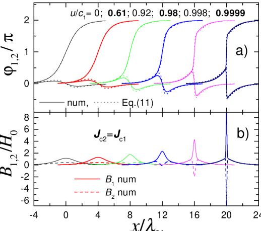
Figure 1: Fluxon shapes in double SJJ’s for different fluxon velocities: a) Solid and dotted lines represent numerical and analytic solutions, respectively, for $\varphi_{1,2}$. b) Magnetic inductions $B_{1,2}$ obtained numerically. The existence of contracted and uncontracted components and the sign inversion of $B_{2}(0)$ at $u\rightarrow c_{1}$ is clearly seen. From Ref. [25].

Apart from the multi-component, two other solutions were predicted in Ref. [20] for double SJJ’s: (i) the single component solution, $sin(\varphi_{1})\simeq\kappa sin(\varphi_{2})$; and (ii) a combination of the single component solution with a traveling plasma wave. Numerical modeling showed [26] that both solutions can be realized at high fluxon velocities. The latter solution was independently discovered in Ref. [55] and was interpreted as ”Cherenkov radiation” from a rapidly moving fluxon.

3.1 Approximate fluxon solution

Let’s consider arbitrary stack of $N$ junctions with a single fluxon in junction $i_{0}$. The problem with solving CSGE, Eq.(4), is coupling of nonlinear $sin(\varphi_{i})$ terms in the right-hand side. Partial linearization with respect to $\varphi_{i\neq i_{0}}$ was proposed in Refs.[25, 32] for decoupling of CSGE. First Eq.(4) is diagonalized to

$$\lambda_{m}^{2}F_{m}^{\prime\prime}=sin(F_{m})+Er_{m},$$ (8)

$$F_{m}=\varphi_{i_{0}}+\sum\kappa_{m,i}\varphi_{i\neq i_{0}},$$ (9)

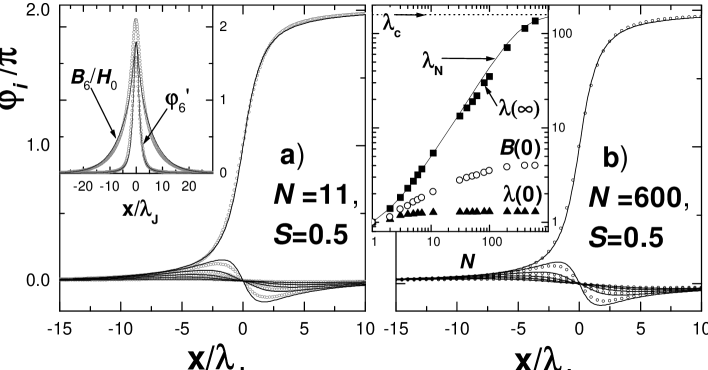
Figure 2: Phase distribution for a fluxon in a) $N$=11 and b) 600 SJJ’s. Circles and lines represent numerical and analytic solutions, respectively. Insets show a) variation of magnetic induction and the derivative of phase in the central JJ; b) variation of characteristic parameters of the fluxon vs. the number of SJJ’s. Data from Ref. [32]

where $Er_{m}=sin(\varphi_{i_{0}})+\sum\kappa_{m,i}sin(\varphi_{i\neq i_{0}})-sin(\varphi_{i_{0}}+\sum\kappa_{m,i}\varphi_{i\neq i_{0}})$. Characteristic lengths, $\lambda_{m}^{-2}$ and coefficients $\kappa_{m,i}$ are given by eigenvalues and eigenvectors of ${\bf A}$, respectively. The diagonalization procedure minimizes error functions, $Er_{m}$ far from the center. In this case $Er_{m}\sim\varphi_{i}^{3}$, while any other linear combination would yield $\sim\varphi_{i}$. Therefore, $Er_{m}$ have a form of small ripple and vanish both inside and far from the fluxon center. In the first approximation $Er_{m}$ terms in Eq.(8) can be neglected, leading to a set of decoupled sine-Gordon equations for $F_{m}$ with well known solutions:

$$F_{m}=4arctan\left(e^{x/\lambda_{m}}\right).$$ (10)

Finally, inverting Eq.(9) we obtain the approximate fluxon solution [25, 32] :

$${\bf\varphi}={\bf K}^{-1}F_{m}(\lambda_{m}),$$ (11)

where ${\bf K}$ is the $N\times N$ matrix with elements equal to $\kappa_{m,i}$. For identical SJJ’s eigenvalues/vectors are given by [19, 24],

$$\lambda_{m} = \lambda_{J}\left[1+2Scos\left(\frac{\pi m}{N+1}\right)\right]^{-1/2},\ m=1,2,\ldots N,$$ (12)

$$\kappa_{m,i} = \left(-1\right)^{i-i_{0}}\frac{sin\left[\pi mi/\left(N+1\right)\right]}{sin\left[\pi mi_{0}/\left(N+1\right)\right].}$$ (13)

Here $S=S_{i}/\Lambda_{i}$ is the coupling parameter, $S=0\div 0.5$. Normalization of eigenvectors in Eq.(13) follows from Eq.(9) and ensures that the total phase shift is $2\pi$ for $i=i_{0}$ and zero for the rest of the junctions.

For SJJ’s with odd $N$ and a fluxon in the middle junction, $i_{0}=N/2$, the number of components reduces to $n=(N+1)/2$, due to a symmetry relation, $\varphi_{i_{0}-j}=\varphi_{i_{0}+j}$, and the solution becomes particularly simple:

$$\varphi_{i_{0}} = \frac{2}{N+1}\sum F_{m}\text{ }\left(m=1,3,\ldots N\right),$$ (14)

$$B_{i_{0}} = \frac{H_{0}}{N+1}\sum\lambda_{m}^{2}F_{m}^{\prime}.$$ (15)

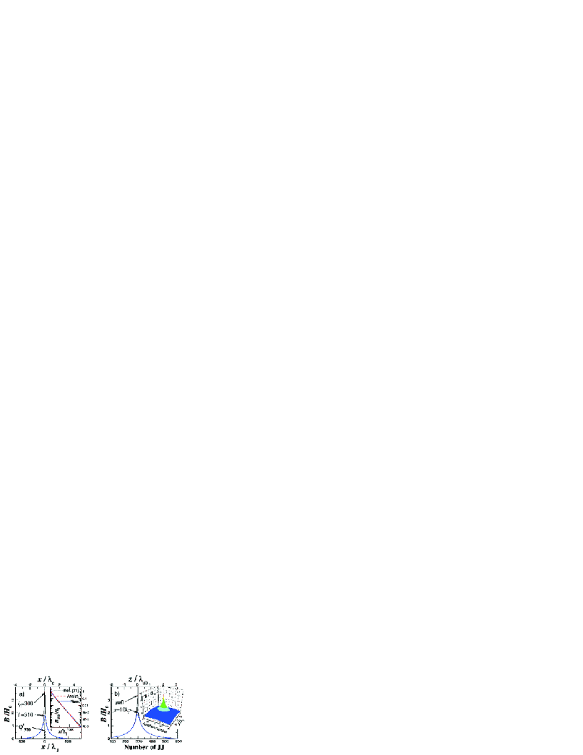
Figure 3: Numerically simulated distributions of magnetic induction for the fluxon in $N$=600 SJJ’s: a) $B(z=const)$ along the $ab$-plane. Dashed line shows the derivative of phase in the central junction. Inset represents comparison between numerical, multi-component and elliptic[14] solutions in the central junction. b) $B(x=const)$ along the $c$-axis. Inset represents a 3D plot of $B(x,z)$ in the fluxon core region. From Ref. [32]

Here are examples of fluxon solutions for small $N$:

$$N=2:\left\{\begin{array}[]{c}\varphi_{1}=\frac{F_{1}+F_{2}}{2},\lambda_{1}=\lambda_{J}\left(1+S\right)^{-1/2}\\ \varphi_{2}=\frac{-F_{1}+F_{2}}{2},\lambda_{2}=\lambda_{J}\left(1-S\right)^{-1/2}\end{array}\right.$$

$$N=3:\left\{\begin{array}[]{c}\varphi_{2}=\frac{F_{1}+F_{3}}{2},\lambda_{1}=\lambda_{J}\left(1+\sqrt{2}S\right)^{-1/2}\\ \varphi_{1,3}=\frac{-F_{1}+F_{3}}{2\sqrt{2}},\lambda_{3}=\lambda_{J}\left(1-\sqrt{2}S\right)^{-1/2}\end{array}\right.$$

$$N=5:\left\{\begin{array}[]{c}\varphi_{3}=\frac{F_{1}+F_{3}+F_{5}}{3},\lambda_{1}=\lambda_{J}\left(1+\sqrt{3}S\right)^{-1/2}\\ \varphi_{2,4}=\frac{-F_{1}+F_{5}}{2\sqrt{3}},\lambda_{3}=\lambda_{J}\\ \varphi_{1,5}=\frac{F_{1}-2F_{3}+F_{5}}{6},\lambda_{5}=\lambda_{J}\left(1-\sqrt{3}S\right)^{-1/2}\end{array}\right.$$

A characteristic feature of the multi-component solution is that the fluxon is characterized by $N$ lengths, $\lambda_{m}$, different from the two lengths of the in elliptic solution [12, 14, 15]. The approximate fluxon solution for the dynamic CSGE, Eq.(5), is given by the same expression, Eq.(11), but with renormalized characteristic lengths,

$$\tilde{\lambda}_{m}^{2}=\lambda_{m}^{2}(1-(\frac{u}{c_{m}})^{2}),$$ (16)

with characteristic velocities [19, 24]

$$c_{m}=c_{0}\left[1+2Scos\left(\frac{\pi m}{N+1}\right)\right]^{-1/2},\ m=1,2\ldots N.$$ (17)

Here $c_{0}=c\sqrt{t/\varepsilon_{r}\Lambda}$ is Swihart velocity for a single junction.

In Fig. 1 spatial distributions of a) phase and b) magnetic induction are shown for a fluxon in two strongly coupled ($S=0.495$) identical SJJ’s at different velocities. Parameters of the stack are: $d_{1-3}=t_{1,2}=0.01\lambda_{J}$, $\lambda_{S1-3}=0.1\lambda_{J}$. A quantitative agreement between ”exact” and approximate solutions is seen. For identical double SJJ’s exactly one half of the fluxon belongs to each of the components, $F_{1,2}$. Indeed, from Fig. 1 a) it is seen that for $u\simeq c_{1}$ there is a Lorentz contracted core at $x=0$ with one-$\pi$ step in $\varphi_{1}$. On both sides of the core, there are two $\pi/2$ tails, decaying at distances $\sim\widetilde{\lambda}_{2}\gg\widetilde{\lambda}_{1}$. Fig. 1 b) represent numerically simulated profiles of $B_{1,2}(x)$. It is seen that the fluxon shape becomes unusual in dynamic state: a dip in $B_{2}$ develops in the center of the fluxon with increasing velocity and at $u\rightarrow c_{1}$ $B_{2}(0)$ changes sign. At $u=c_{1}$, $B_{2}(0)=-B_{1}(0)$, in agreement with the multi-component solution.

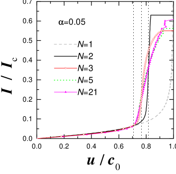
Figure 4: Numerically simulated current-velocity characteristics for a single JJ $N=1$ (dashed line), and for SJJ’s with different $N$: $N=2$ (solid line), $N=3$ (open circles), $N=5$ (dotted line) and $N=21$ (filled triangles). From Ref.[32]

Numerically simulated fluxon profiles for $N=$11 and 600 SJJ’s are shown in Figs. 2 and 3. Parameters are typical for Bi2212: $d$=3 Å, $t$ =12 Å, $\lambda_{J}=1\mu m$ ($J_{c}\simeq 675A/cm^{2}$), $\lambda_{s}$=750 Å($\lambda_{ab}\simeq 0.17\mu m$). It was shown that the multi-component solution correctly describes the fluxon shape in static case for arbitrary SJJ [20, 25, 26, 32].

3.2 Decoupling of phase and field

Inset in Fig. 2 a) shows spatial variation of $B$ and $\varphi^{\prime}$ in the central JJ $i_{0}$=6 of $N=11$ SJJ’s. It is seen that length scales for variation of $\varphi$ and $B$ are different: $\varphi$ varies at distances $\simeq\lambda_{J}$, while the characteristic length for variation of $B$ at large distances, $\lambda(\infty)$, is $\lambda_{11}=5.4\lambda_{J}$, Eq.(12). The discrepancy between $\varphi_{i_{0}}^{\prime}$ and $B_{i_{0}}$ becomes dramatic for large $N$, see Fig. 3 a). This is in sharp contrast with behavior of Josephson vortices in single JJ’s or Abricosov vortices in type-II superconductors, in which spatial variations of both phase/current and magnetic induction are given by the same length scale. Existence of one and the same length scale for $I$ and $B$ is viewed as a natural consequence of Ampere’s law.

So, how could phase/current decouple from magnetic induction in SJJ’s? This can be understood from the multi-component fluxon solution: (i) Magnetic induction in SJJ’s is non-local, $B_{i}$ depends on $\varphi_{i}$ in all junctions, see Eq.(3), which is an essence of magnetic coupling. (ii) If the fluxon has a multi-component structure, then distribution of phase is determined by the shortest, while magnetic induction - by the longest characteristic length. Indeed, according to Eq. (14), the effective Josephson penetration depth in the center of the fluxon is

$$\lambda(0)=\frac{2}{\varphi_{i_{0}}^{\prime}(0)}\simeq\frac{n}{\sum\lambda_{m}^{-1}},$$ (18)

which is obviously dominated by the shortest length $\lambda_{1}\sim\lambda_{J}$. On the other hand, from Eq. (15), variation of $B$ is dominated by the longest length, $\lambda_{N}$, which according to Eq. (12) increases rapidly with $N$ for strongly coupled SJJ’s, $S\rightarrow 0.5$.

3.3 N-dependence and assymptotics

Fluxon shape strongly depends on the number of junctions in a stack. Inset in Fig. 2 b) summarizes variation of the fluxon shape for different $N$. Open circles represent magnetic induction at the center of the fluxon $B(0)$. $B(0)$ increases with $N$ and saturates at $B(0)\simeq 4H_{0}$ for $N>\lambda_{ab}/s$. Triangles represent numerically obtained $\lambda(0)$, which characterize variation of phase/current in the fluxon core. In agreement with Eq. (18), $\lambda(0)$ increases only slightly with $N$ and saturates at $\simeq 1.3\lambda_{J}$ for $N>10$. On the other hand, the effective magnetic length far from the core, $\lambda(\infty)$, increases dramatically with $N$. $\lambda(\infty)$ is determined by the largest characteristic length $\lambda_{N}$, as shown by the solid line. For large $N>\lambda_{ab}/s$, $\lambda_{N}\rightarrow\lambda_{c}$, see dotted line in inset of Fig.2 b), and the multi-component solution approaches the elliptic solutions [12, 14]. This is demonstrated in inset of Fig. 3 a). Top axes in Figs. 3 a) and b) show that $B(x,z)$ varies at length scales $\sim\lambda_{c}$ and $\lambda_{ab}$ along and across layers, respectively. It is also seen that the most spectacular feature of the fluxon is a sharp peak $B(0,0)$, representing the ”Josephson core” of the fluxon $\sim\lambda_{J}\times s$ in $ab$-plane and $c$-axis, respectively, as shown in inset of Fig. 3 b).

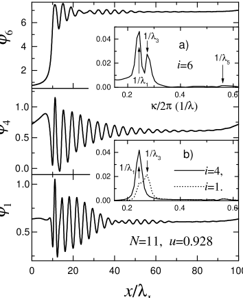
Figure 5: Phase distributions for the fluxon moving with velocity $u\simeq 0.928c_{0}$ in $N=11$ SJJ’s are shown for the central junction, $i=6$, (top panel); $i=4$ (middle panel); and $i=1$ (bottom panel). Spectra of Cherenkov radiation are shown in insets a) for $i=6$ and b) for $i=4$ (solid line) and $i=1$ (dotted line). From Ref. [32].

Since the fluxon has several characteristic lengths, a question may arise, what is the effective Josephson penetration depth, $\lambda_{J(eff)}$. This is important to know, because behavior of SJJ’s changes drastically when $L>\lambda_{J(eff)}$. Roughly speaking, fluxons can exist only in ”long” JJ’s, $L\gg\lambda_{J(eff)}$, causing a large difference in behavior of ”short” and ”long” JJ’s. Length scales somewhat different from that in [14] were derived in Ref. [18], based on simulations for $N=15$. In general, different conclusions about the fluxon size could be made from numerical simulations for different $N$: short scale $\sim\lambda_{J}$ for $N$=7 [4], and $N$=19 [19]; and long scale $\sim\lambda_{c}$ for $N$=50 [21]. Long scale, $\sim\lambda_{c}$, variation of $B$ for $N>1000$, was deduced from experimental observations of the fluxon in HTSC [56]. From the analysis above it is clear that such ”discrepancy” is a consequence of strong $N-$ dependence of the fluxon shape, however, $\lambda_{J(eff)}=\lambda(0)$ is always $\simeq\lambda_{J}$, as shown in inset of Fig. 2 b).

3.4 Flux-flow characteristics

Variation of fluxon shape in dynamic state is particularly interesting both because it has a direct impact on $c-$axis transport properties and because fluxon shape becomes very unusual at high propagation velocities, see Fig. 1. When bias current is applied, a fluxon starts moving along the junction with a velocity determined by the balance between Lorentz and viscous friction forces. This results in appearance of a flux-flow branch in current-voltage characteristics (IVC’s) with average DC voltage $V_{i_{0}}/V_{0}=u/c_{0}$, ($V_{0}=\frac{\hbar\pi c_{0}}{2eL}$) in the JJ containing the fluxon and zero for $i\neq i_{0}$. Therefore, current-velocity characteristics are equivalent to IVC’s. In a single JJ, fluxon is a relativistic object. It gets Lorentz contracted [57] when the fluxon velocity approaches Swihart velocity, i.e. the phase velocity of electromagnetic waves in the transmission line formed by the junction. However, in SJJ’s according to the multi-component solution, only $F_{1}$ component of the fluxon gets Lorentz contracted at the lowest velocity $c_{1}$. The weight of this component decreases with $N$, i.e., there is less contraction for larger $N$.

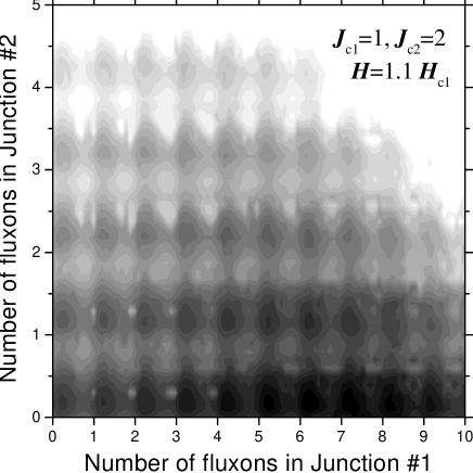
Figure 6: Gray scale plot of Gibbs free energy versus the number of fluxons in double SJJ’s at $H=1.1H_{c1}$. Darker regions correspond to smaller Gibbs energy. The existence of multiple quasi-equilibrium states is seen. From Ref. [20].

So, what happens with the fluxon in SJJ’s: does it gets contracted at $u=c_{1}$ or not? Systematic analysis of the double SJJ’s showed that the answer strongly depends on parameters of SJJ’s [26]. From Fig. 1 it is seen that the fluxon in identical double SJJ’s is well described by the multi-component solution up to $u=c_{1}$. However, in general, partial linearization procedure fail at $u=c_{1}$ because $\varphi_{i\neq i_{0}}$ is no longer small. It was found [26], that for $\frac{J_{c2}\Lambda_{2}}{J_{c1}\Lambda_{1}}>1$ and $\kappa_{2}>1$, a ”single component” ($F_{2}$) solution [20] is realized in double SJJ’s. This solution was anticipated in Ref. [20] and is characterized by relationship $sin(\varphi_{1})\simeq\kappa_{2}sin(\varphi_{2})$. Note, that it becomes exact at $u=c_{1}$ for the above mentioned parameters. Apparently, the single $F_{2}$ component fluxon does not contract at $u=c_{1}$.

In Fig. 4, numerically simulated IVC’s are shown for a single junction $N=1$, and SJJ’s with $N=$2, 3, 5 and 21. Simulations were done for annular junction geometry with $L=100\lambda_{J}$, parameters typical for Bi2212 HTSC and damping coefficient $\alpha_{i}=0.05$. Vertical dotted lines represent lowest characteristic velocities: $c_{1}(N=2)\simeq 0.8165$, $c_{1}(N=3)\simeq 0.7653$ and $c_{1}(N=21)\simeq 0.7071c_{0}$. Clear velocity matching step at $u\rightarrow c_{0}$ is seen for a single junction [58]. Vertical portions of IVC’s at $u\rightarrow c_{1}$ are also seen for $N=$ 2 and 3, as a result of partial Lorentz contraction of the fluxon, see Fig. 1. However, for $N=5$ and 21 there is no peculiarity in IVC’s at a velocity matching condition $u=c_{1}$, indicating absence of fluxon contraction. In Ref. [32] it was found out that Lorentz contraction at $u=c_{1}$ is absent for SJJ’s with $N>3$. Note that there are very little changes in IVC’s for $N\geq 5$ (the IVC’s for $N=5$ and 21 are almost indistinguishable in Fig. 4). This is due to the fact that dissipation is mostly determined by the fluxon core region, which remains almost unchanged for $N\geq 5$, see $N-$dependence of $\lambda(0)$ in inset of Fig. 2 b).

3.5 Cherenkov radiation

Due of the lack of Lorentz contraction, the fluxon can propagate with a velocity larger than $c_{1}$ as independently proposed in Refs. [55, 20]. Such super-relativistic motion is accompanied by ”Cherenkov” radiation [13, 55, 26, 31, 32, 59]. An important insight to Cherenkov radiation can be obtained from the multi-component solution. For $u>c_{n}$, characteristic lengths $\tilde{\lambda}_{m<n}$ become imaginary, characteristic for ”wave” solutions. Indeed, far from the fluxon center we can further linearize Eq.(8), and obtain that the solution for $F_{m<n}$ is a traveling wave with the dispersion relation [20, 32]:

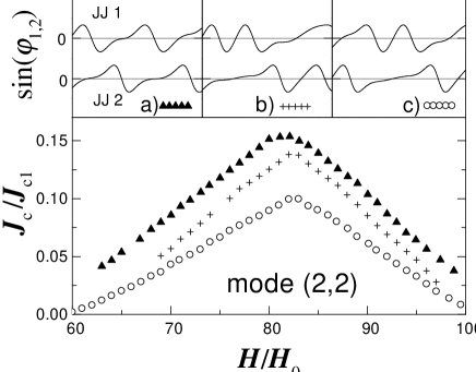
Figure 7: Three simulated $I_{c}(H)$ sub-branches of double SJJ’s, corresponding to submodes of the (2,2) mode with different fluxon sequence. Insets a-c) show spatial current distributions in junctions 1 and 2 for each submode at $H/H_{0}=80$. From Ref. [23]

$$\kappa_{m}^{-2}=u^{2}/\tilde{\omega}_{p}^{2}-\lambda_{m}^{2},\ \omega=u\kappa_{m},$$ (19)

where $\tilde{\omega}_{p}^{2}=\omega_{p}^{2}\sqrt{1-J_{b}^{2}}$. Those are Josephson plasma waves [19, 24] moving along with the fluxon at velocity $u$ [20].

In Fig. 5, numerically simulated phase distributions for a rapidly moving fluxon ($c_{6}>u\simeq 0.928c_{0}>c_{5}$) in $N=11$ SJJ’s are shown for a central junction, containing the fluxon, $i_{0}=6$ (top panel); $i=4$ (middle panel); and the outmost junction $i=1$ (bottom panel). Parameters of SJJ’s are the same as in Fig. 4. The six lowest characteristic velocities for $N=11$ are $c_{1}=0.7132c_{0}$, $c_{2}=0.7320c_{0}$, $c_{3}=0.7653c_{0}$, $c_{4}=0.8165c_{0}$, $c_{5}=0.8913c_{0}$, $c_{6}=c_{0}$. Well defined oscillations are seen behind the fluxon (the fluxon is moving from right to left). The spectra of oscillations are shown in insets a) for $i=6$ and b) for $i=4$ (solid line) and $i=1$ (dotted line). Clear beatings of oscillations are seen in JJ’s 6 and 1, which is a signature of coexistence of multiple wave lengths. Indeed, spectra of oscillations exhibit several maxima corresponding to odd plasma modes, as indicated by arrows in insets a and b).

Numerical simulations support the assumption [20] that Cherenkov radiation at $u>c_{n}$ is due to degeneration of fluxon components $F_{m<n}$ into Josephson plasma waves [26, 32]. Namely, it was observed that: (i) Plasma mode $m$ is generated when $u>c_{m}$. (ii) Only those modes which constitute the fluxon, appear in Cherenkov radiation. E.g., for a fluxon in the central junction of a stack with odd $N$ there are no even modes, see Eq. (14) and Fig. 5. (iii) Relative amplitudes of oscillations are related to weights coefficients of the corresponding fluxon component. For the case of Fig. 5, weight coefficient of mode 3 in junction 4, $K^{-1}_{4,3}=0$, and plasma mode 3 is absent in the spectrum. On the contrary, for the outmost junction, the weight coefficient of mode 3, $K^{-1}_{1,3}\simeq 0.118$, is significantly larger than for mode 1, $K^{-1}_{1,1}\simeq-0.043$, and the maximum of amplitude corresponds to plasma mode 3, see inset b) in Fig. 5.

4 MULTI-FLUXON CONFIGURATIONS

Due to repulsive fluxon interaction, fluxons are believed to form a regular fluxon lattice (FL) at large parallel magnetic field. Since magnetic induction of a fluxon is spread over many layers, see Fig. 3, it is not favorable to have a perfect translational symmetry along the $c-$axis, and FL is expected to be rhombic [60]. However, the perfect FL can be achieved only when fluxons strongly interact with each other, i.e., when spacing between fluxons along the $ab$-plane is $\sim\lambda_{J}$. For Bi and Tl based HTSC, the corresponding magnetic field, $\Phi_{0}/\lambda_{J}s\sim$ 1T is three orders of magnitude larger than the lower critical field $H_{c1}^{\mid\mid}\sim$mT [33, 34].

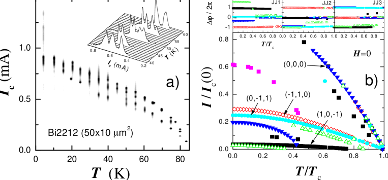
Figure 8: a) A gray scale plot of the probability distribution of $I_{c}(T)$ for a Bi2212 mesa. Inset demonstrates multiple-peak structure of $P\left(I_{c}\right)$ for several $T$. b) Simulated $I_{c}(T)$ for three SJJ’s with Bi2212 parameters at $H$=0. Multiple $I_{c}(T)$ branches are clearly seen. Branches corresponding to (0,0,0) and simplest fluxon-antifluxon modes are marked. Insets show distribution of fluxons in the stack. From Ref. [30]

Fluxon distribution in layered superconductors at low fields, $H_{c1}^{\mid\mid}<H<\Phi_{0}/\lambda_{J}s$, is still a matter of controversy. Levitov [60] have found ”phyllotaxis” and bifurcations in the FL at low fields, due to existence of multiple metastable FL’s with approximately equal energies. In Ref. [61], this approach was extended using a ”growth” algorithm, allowing variation of the FL along the $c$-axis. Although restricted to constant space periodicity along layers, the model showed the existence of a large variety of quasi-periodic or aperiodic fluxon configurations in the $c$-axis direction. At low fields, the fluxon system becomes completely frustrated and tends to be chaotic [61]. Recent numerical simulations revealed that fluxons in SJJ’s may form buckled chains [21, 22] instead of the regular FL. Clearly, the lattice description of multi-fluxon distribution becomes unappropriate at low magnetic fields.

4.1 Quasi-equilibrium fluxon modes and submodes

Recently it was shown that multiple quasi-equilibrium fluxon configurations (modes) exist in long, $L\gg\lambda_{J}$, strongly coupled SJJ’s [20]. Fig. 6 shows a numerically simulated gray scale plot of Gibbs free energy versus the number of fluxons in double SJJ’s for applied parallel field slighltly above the lower critical field, $H=1.1H_{c1}$. Parameters of the stack are $J_{c2}=2J_{c1}$, $\lambda_{Si}=0.1\lambda_{J1}$, $t_{i}=d_{i}=0.01\lambda_{J1}$, $L=50\lambda_{J1}$. Darker regions correspond to smaller Gibbs energy. The absolute minimum, representing a thermodynamic equilibrium, correspond to 7 fluxons in junction 1 and zero fluxons in junction 2. However, it is seen that there is a number of other fluxon configurations (modes) for which local minima of Gibbs free energy is achieved. All those modes are stable and represent quasi-equilibrium states of the stack. The modes are characterized by different fluxon distributions in the stack and do not have $a-priori$ any translational symmetry. We will use a string $(n_{1},...n_{i},...n_{N})$ as a short notation of fluxon modes, where $n_{i}$ is a number of fluxons in junction $i$ and $N$ is the number of junctions in the stack. E.g., the equilibrium state in Fig. 6 corresponds to (7,0) mode.

In Ref. [23] existence of fluxon submodes was demonstrated, which have the same number of fluxons but are different with respect to fluxon sequences and symmetry of phase differences in the junctions (along the planes). Insets a-c) in Fig. 7, show three different submodes of (2,2) mode for a double stack with the same parameters as in Fig. 6. Those submodes have nearly equal self energies, i.e. nearly equal probability, however, correspond to distinctly different $I_{c}(H)$ sub-branches.

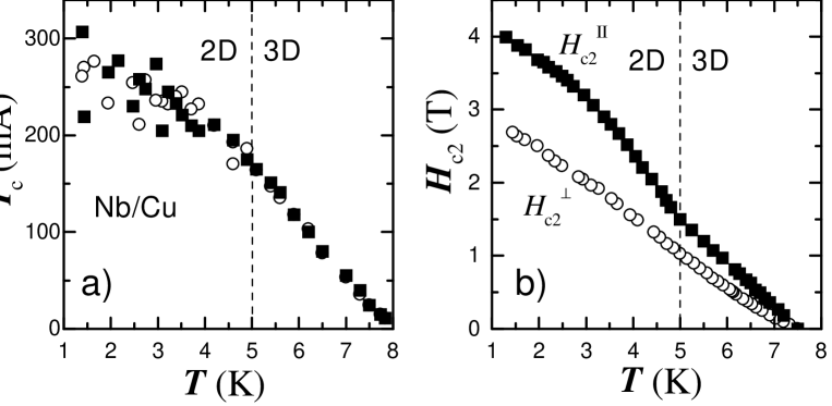
Figure 9: a) $I_{c}\left(T\right)$, for Nb/Cu multilayer. Different symbols correspond to different runs. It is seen that strong fluctuations of $I_{c}$ take place in the 2D state. b) The upper critical field parallel (solid rectangles) and perpendicular (open circles) to layers. A kink in $H_{c2}^{\mid\mid}$ represents the 3D-2D crossover. Data from Ref. [30]

The number of fluxon modes and submodes increases rapidly with increasing number of junctions and fluxons. From mathematical statistics it follows that for a stack with N non-identical junctions with M fluxons, the total number of fluxon modes (indistinguishable fluxon sequences) is

$$N_{modes}=\frac{(N+M-1)!}{(N-1)!M!},$$ (20)

and the number of submodes (distinguishable fluxon sequences) is

$$N_{submodes}=N^{M}.$$ (21)

A specific feature of SJJ’s is existence of stable fluxon-antifluxon pairs [30]. Due to attractive interaction between fluxons and antifluxons, they tend to collapse both in a single junction or type-II superconductor. However, in SJJ’s fluxons can not move across S-layers. Therefore, a fluxon and an antifluxon in neighbor junctions do not collapse, but form a bound pair. Furthermore, once in the stack, such pair can not be removed (unless destroyed) by transport current because there is no net Lorentz force on the pair. Fluxon-antifluxon pairs are likely to be present in SJJ’s at $H<H_{c1}$ and can dominate transport properties at zero field [30, 31].

Due to existence of multiple quasi-equilibrium fluxon (and fluxon-antifluxon) modes/ submodes, the state of SJJ’s is not well defined. It can be described only statistically with a certain probability of being in any of the modes. Neither the number of fluxons in each junction nor even the total number of fluxons in the stack is fixed for given $H$ and $T$. Moreover, since different fluxon modes/submodes may have similar energies, the system is frustrated and exhibit strong fluctuations. This may account for unusual $c$-axis transport properties of both HTSC mesas [62, 23, 30] and low-$T_{c}$ SJJ’s [53, 30].

4.2 Multiple-valued critical current

Statistical analysis is crucial for probing multiple quasi-equilibrium states in SJJ’s. Fig. 8 a) presents in a gray scale a probability distribution of critical current $P\left(I_{c}\right)$ vs. $T$ for 50 $\mu$m long Bi2212 mesa with $N=5$ intrinsic SJJ’s, at earth magnetic field. Darker regions correspond to a larger probability. To obtain $P\left(I_{c}\right)$, 5120 switching events from zero-voltage state were measured at each $T$ [62, 30]. Inset in Fig. 8 a) shows $P\left(I_{c}\right)$ for 40 K $<T<$ 60 K. It is seen that $P\left(I_{c}\right)$ is very wide and consists of several superimposed peaks, attributed to different fluxon modes [62, 30].

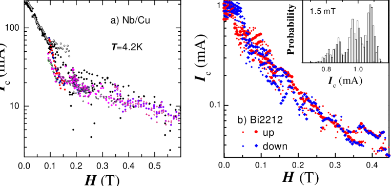
Figure 10: $I_{c}(H)$ dependencies for a) Nb/Cu multilayer, and b) Bi2212 mesa. Symbols correspond to maxima in $P(I_{c})$, shown in inset. Data from Ref. [30]

In Fig. 8 b) simulated $I_{c}(T)$ dependencies are shown for $N=3$ long ($L=10\lambda_{J}$) SJJ’s with Bi2212 parameters, at $H$=0. Different symbols represent separate runs with increasing or decreasing $T$ and/or different initial conditions. It is seen that $I_{c}(T)$ consists of multiple distinct branches, in qualitative agreement with experiment. Insets in Fig. 8 b) show amount of fluxons in the junctions. It can be seen that each $I_{c}(T)$ branch corresponds to a particular fluxon or fluxon-antifluxon mode. I want to emphasize that $I_{c}$ is multiple valued even at $H=0$. This is due to stability of fluxon-antifluxon pairs in SJJ’s as discussed above. Branches corresponding to simplest fluxon-antifluxon modes (-1,1,0), (0,-1,1) and (1,0,-1) are marked in Fig. 8 b).

Fig. 9 a) shows $I_{c}\left(T\right)$ for a Nb/Cu (20/15 nm $N=$ 10) multilayer. Different symbols correspond to different runs. Measurements were done at $H\sim$ 10 mT along layers. It is seen that $I_{c}$ strongly fluctuates below $\sim$5 K. Fig. 9 b) shows the upper critical field $H_{c2}(T)$ parallel (solid rectangles) and perpendicular (open circles) to layers. A kink in $H_{c2}^{\mid\mid}(T)$ reflects dimensional 3D-2D crossover, which is well studied in those systems [48,53,63-66]. The 3D-2D crossover is one of peculiar properties of superconducting multilayers [67]. In the 3D state a multilayer behaves as a bulk superconductor, while in the 2D state - as a stack of Josephson junctions [48, 53]. Dashed lines in Fig. 9 show, that strong fluctuations of $I_{c}$ appear in the 2D state reflecting appearance of SJJ’s. This unambiguously demonstrates that multiple valued critical current is a genuine feature of SJJ’s, due to existence of multiple fluxon modes.

4.3 Magnetic field dependence of the critical current

The dependence of $I_{c}$ on in-plane magnetic field is a crucial test for dc Josephson effect. In a single JJ, Fraunhofer modulation of $I_{c}(H)$ occurs as a result of flux quantization [68]. For SJJ’s it was predicted that the periodicity of $I_{c}(H)$ is [69]

$$\Delta H=\Phi_{0}/Ls.$$ (22)

However, experimental $I_{c}(H)$ both for HTSC [70, 71, 23] and low-$T_{c}$ [45, 49, 72, 53] SJJ’s do not show such periodicity. So, what’s wrong with dc-Josephson effect in SJJ’s?

Experimental $I_{c}(H)$ for Nb/Cu multilayer ($N$=10, $L=$20 $\mu$ m) and Bi2212 mesa ($N=$5, $L=$ 20 $\mu$m) are shown in Fig. 10 a) and b), respectively, at $T=$ 4.2 K. Note a logarithmic scale of $I_{c}$. In Fig. 10 a), different symbols represent different zero- field-cooled runs with increasing field. Fig. 10 b) shows a result of statistical analysis. Large and small symbols in Fig. 10 b) represent main and secondary peaks in $P(I_{c})$, respectively, for increasing (circles) and decreasing (diamonds) field. The probability distribution with several maxima is shown in inset. It is seen that $I_{c}$ is multiple valued and, even though one could probably recognize certain branches, there is no periodic Fraunhofer modulation.

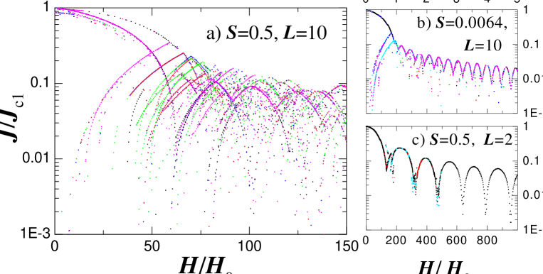
Figure 11: Simulated $I_{c}(H)$ for a) long, strongly coupled b) long, weakly coupled and c) short, strongly coupled double SJJ’s. It is seen that Fraunhofer modulation is obscured in long, strongly coupled SJJ’s due to existence of multiple quasiequilibrium fluxon modes. However, periodicity of $I_{c}(H)$ is restored either in weakly coupled or short SJJ’s. Data from Ref. [23]

Fig. 11 presents numerically simulated $I_{c}(H)$ patterns for a) long strongly coupled ($L=10\lambda_{J1}$, $S=0.495$, $d/\lambda_{S}=0.1$); b) long weakly coupled ($L=10\lambda_{J1}$, $S=0.0064$, $d/\lambda_{S}=5$) and c) short strongly coupled ($L=2\lambda_{J1}$, $S=0.495$, $d/\lambda_{S}=0.1$) double SJJ’s with $J_{c2}=2J_{c1}$. Note logarithmic scale for $I_{c}$. Plots contain several runs for increasing or decreasing field with different initial conditions. From Fig. 11 a) it is seen that the $I_{c}(H)$ pattern for long, strongly coupled SJJ’s consists of multiple closely spaced branches. Each branch is characterized by a certain fluxon distribution, i.e., corresponds to a certain fluxon mode or submodes, see Fig. 7. The $I_{c}(H)$ pattern does not exhibit clear periodicity because $I_{c}$ switches randomly between closely spaced branches. This does not mean that something is wrong with dc Josephson effect, but rather is a consequence of magnetic coupling between junctions.

From Figs. 11 b) and c) it is seen that periodicity of $I_{c}(H)$ is restored either when the coupling is decreased or a stack becomes short compared to $\lambda_{J}$. For weakly coupled SJJ’s, $I_{c}(H)$ is simply determined by the smallest critical current of individual JJ’s, while in short SJJ’s there are no fluxons and, consequently, no fluxon modes. A transition from aperiodic to periodic modulation of $I_{c}(H)$ with decreasing $L/\lambda_{J}$ was observed both for Nb/Cu multilayers [53] and for YBa₂Cu₃O_7-x [73] close to $T_{c}$.

4.4 Multiple flux-flow sub-branches

In sec. 3.4 we considered viscous motion of a single fluxon. For a multi-fluxon configuration, time averaged flux-flow voltage is proportional to the number of fluxons in SJJ’s and a fluxon velocity. For large $H$, the ratio $V/H$ is:

$$V/H\simeq Nsu.$$ (23)

Note that it is independent on the junction length. A characteristic feature of SJJ’s is splitting of Swihart velocities, see Eq.(17), and corresponding splitting of flux-flow IVC’s [4, 19, 24]. Flux-flow phenomenon was intensively studied both for HTSC [30,37-41,74,75] and low-$T_{c}$ [47, 50, 54] SJJ’s due to possible application as a source of microwave radiation [27]. From application point of view, the most interesting is coherent (in-phase) fluxon propagation [4] at the highest characteristic velocity $c_{N}$, because it could generate narrow linewidth radiation with large amplitude [27]. However, so far the measured radiation linewidth from SJJ’s was much wider than expected [76, 55].

In Fig. 12 a) flux-flow IVC’s of long ($L=50\mu$m, $N=5$) Bi2212 mesa are shown for $H=0.148-0.396$ T with a step $\simeq$ 0.025 T, at $T$=4.2 K. Magnetic field was applied along the $ab$-plane and perpendicular to the longest side of the mesa. It is seen, that a low resistance branch develops in IVC’s with increasing $H$. The 20 $\mu$m long mesa on the same single crystal showed the same $V/H$ value, in agreement with Eq. (23). However, IVC’s were more complicated due to presence of Fiske steps [41]. The maximum flux-flow velocity is close to the lowest characteristic velocity $c_{1}\simeq 2.5-3\times 10^{7}cm/s$. This value is consistent with observations by different groups [37-41,74,75] and is in agreement with the Fiske step voltage observed in Bi2212 mesas [41].

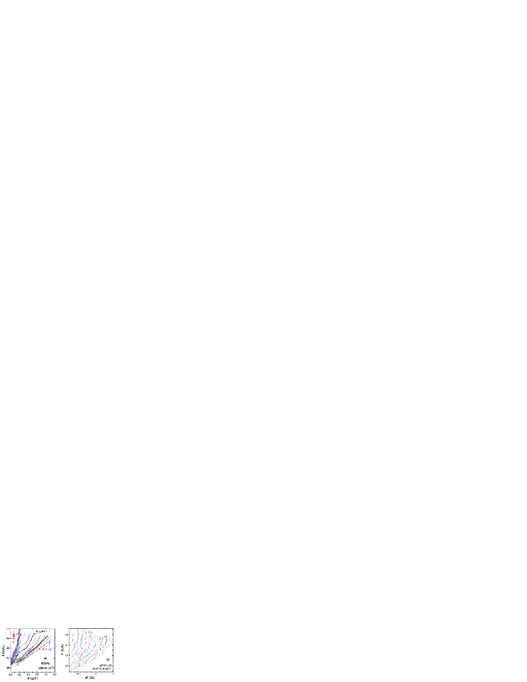
Figure 12: a) Flux-flow IVC’s of 50 $\mu$m long Bi2212 mesa with $N=5$ intrinsic SJJ’s at $T$=4.2 K are shown for $H$ from 0.148 to 0.396 T with a step $\simeq$0.025 T. b) Enlarged top parts of $I$ vs. $R=V/I$ curves are shown for $H$ varying with a small step $\simeq$5 mT in the range $H$=0.351$\div$0.396 T, at $T$=4.2 K. Closely spaced flux-flow sub-branches are seen. Data from Ref. [30]

From Fig. 12 a) it is seen that flux-flow branches exhibit strong fluctuations. At small voltages, the spread in IVC’s reflects fluctuations in $I_{c}$, as discussed in sec. 4.2. In Fig. 12 b) enlarged top parts of $I$ vs. $R=V/I$ curves for the same mesa are shown at magnetic fields in the range 0.351 - 0.396 T, varying in small steps $\simeq$ 5 mT, at $T$=4.2 K. The characteristic feature of IVC’s from Fig. 12 is that the curves are not just uniformly wide, but rather consist of multiple closely spaced but distinct sub-branches. The IVC’s switch hysteretically between sub-branches when current is swept back and forth. Varying $H$, we only change the set of available sub-branches but do not change the shape of a particular sub-branch.

Similar multiple flux-flow sub-branches were observed for Nb/Cu multilayers [53] and HTSC mesas [74, 77]. In the latter two papers it was suggested that sub-branching is due to splitting of Swihart velocities. Indeed such splitting was observed for low-$T_{c}$ SJJ’s [47, 50, 54] and possibly for HTSC mesas [75]. In those cases branches revealed different $V/H$ scaling, corresponding to different $c_{n}$, see Eq.(23). On the contrary, tiny sub-branches shown in Fig.12 b) (as well as those observed in Refs. [74, 77]) have approximately the same $V/H$ scaling corresponding to the lowest velocity $c_{1}$. Furthermore, because of small $N$=5, splitting of $c_{n}$ should correspond to almost two orders of magnitude larger splitting than that in Fig. 12 b) [75]. It should also be noted that the number of sub-branches is not limited by the number of SJJ’s in the mesa. All this rules out explanation of multiple flux-flow sub-branches, shown in Fig. 12 b), in terms of splitting of Swihart velocities.

In Refs. [53] it was proposed that multiple flux-flow sub-branches correspond to propagation of different quasi-equilibrium fluxon modes. This was supported by direct numerical simulations [28, 30, 31]. Fig. 13 presents numerical modeling of IVC’s for the mesa from Fig. 12 ( $N=5$, $J_{c}\sim 10^{3}A/cm^{2}$, $s=15\AA$, $d=3\AA$, $\lambda_{J}\simeq 1\mu m$, $L/\lambda_{J}=50$ and damping parameters $\alpha_{i}=0.05$). Junctions are identical, except for larger thickness of the bottom electrode, $d_{1}=6\AA$, in order to imitate the bulk crystal beneath the mesa. Two successive back-and-forth current sweeps are shown (denoted as A and B) at in-plane magnetic field $H=10^{4}H_{0}\simeq 2000$ Oe. Top three panels show overall IVC’s of the stack, $V=\sum V_{i}$, with successive ”zoom-in” to a small voltage region: panel a) demonstrates IVC’s in a large scale, panel b) presents the flux-flow branch, and panel c) shows details of switching between supercurrent ($V=0$) and flux-flow branches. In the bottom row, the left and right groups of plots represent data for sweeps A and B, respectively. In each group, the left plots represent individual IVC’s of all five junctions (successively shifted along $V-$ axis for clarity), while the right plots show amount of fluxons in each junction, determined as $[\varphi_{i}(L)-\varphi_{i}(0)]/2\pi$ (lines), and the total amount of fluxons in the stack (symbols). Despite nominally the same external conditions, the IVC’s A and B are apparently different. For the IVC-A only three ($i=$2, 3, and 4), while for the IVC-B all five junctions switch to the normal branch (shown by dotted lines in Fig. a)) at the end of the flux-flow branch.

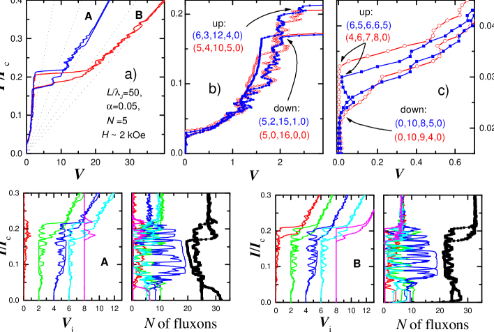
Figure 13: Simulated IVC’s are shown for two back-and-forth current sweeps (denoted as A and B) for the Bi2212 mesa from Fig. 12. Top three panels show overall IVC’s $V=\sum V_{i}$, with successive ”zoom-in” to a small voltage region from panel a) to c). Fluxon modes realized at the end and the beginning of flux-flow branches for both sweeps are specified. In the bottom row, IVC’s of individual junctions (successively offset along the $V-$ axis for clarity) and the number of fluxons in the junctions are shown. It is seen that fluctuation of the flux-flow voltage is due to switching between fluxon modes.

From Fig. 13 b) it is seen that flux-flow branches exhibit strong fluctuations, caused by variation of fluxon numbers in junctions, as shown in the bottom row of Fig.13. Each time fluxons leave the stack on one side, other fluxons entering the stack on the opposite side have freedom to choose between all possible quasi-equilibrium fluxon modes. Each fluxon mode is represented by a distinct flux-flow sub-branch, with slightly different $I_{c}$ and flux-flow voltage. Two of such sub-branches can be seen at $I/I_{c}=0.1-0.15$ in Fig. 13 b). Fluxon modes realized at the end and the beginning of flux-flow branches for both sweeps are specified in Figs. 13 b) and c), respectively. Note that in both cases the maximum fluxon velocity is close to the lowest characteristic velocity $\sim c_{1}$, i.e., splitting of $c_{n}$ is not the cause of sub-branching of IVC’s. Fig. 13 c) demonstrates that critical currents and return currents are also different for the two sweeps, i.e., $I_{c}$ is multiple valued. As discussed in sec. 4.2. different $I_{c}$’s correspond to different modes, indicated in Fig. 13 c).

Fig. 13 reproduces main features of experimental IVC’s from Fig. 12. In Ref. [31] it was shown that tiny sub-branches due to fluxon-antifluxon modes exist also at zero field. Switching between fluxon modes/submodes and correlated fluctuations of flux-flow voltage would cause extremely wide radiation line width, consistent with numerical simulations [27] and experimental radiation detection from HTSC SJJ’s [55].

5 CONCLUSIONS

In conclusion, single and multi-fluxon properties of layered superconductors and stacked Josephson junctions were analyzed. We have seen that behavior of SJJ’s can be qualitatively different from that of single Josephson junctions or type-II superconductors. To a large extent, anomalous properties are due to unusual fluxon shape and existence of multiple quasi-equilibrium fluxon modes in long, strongly coupled SJJ’s.

The single fluxon in the stack of $N$ junctions is described by $N$ characteristic lengths. With increasing velocity, magnetic induction in a fluxon can change sign. For large $N$ there is no Lorentz contraction of the fluxon at $u\rightarrow c_{1}$. This results in absence of velocity matching behavior and a possibility of ”super-relativistic” fluxon motion with $u>c_{1}$. Such motion is accompanied by generation of Josephson plasma waves moving along with the fluxon (”Cherenkov” radiation) due to degeneration of fluxon components with $c_{m}<u$.

Due to existence of multiple quasi-equilibrium fluxon modes/submodes the state of the stack is not well defined for given external conditions. It can only be described statistically with a certain probability of being in any of quasi-equilibrium states. This causes complicated and anomalous behavior of SJJ’s: (i) Characteristics of SJJ’s exhibit strong fluctuations. (ii) The $c$-axis critical current is multiple valued. The probability distribution $P(I_{c})$ has multiple maxima and $I_{c}(T,H)$ consist of multiple sub-branches. (iii) The $I_{c}(H)$ patterns are aperiodic. (iv) Flux-flow IVC’s consist of multiple closely spaced sub-branches.

References

- [1] W.E.Lowrence and S.Doniach, in Proc. LT-12, Kyoto, 1970, ed. by E.Kanada (Keigaku, Tokyo 1970), p.361
- [2] R. Kleiner, F.Steinmeyer, G.Kunkel, P.Müller, Phys. Rev. Lett. 68, 2394 (1992)
- [3] M.B.Mineev, G.S.Mkrtchyan, and V.V.Shmidt, J.Low Temp. Phys. 45, 497 (1981)
- [4] S.Sakai, P.Bodin and N.F.Pedersen, J. Appl. Phys. 73, 2411 (1993)
- [5] T.Koyama and M.Tachiki, Phys. Rev.B 54 (1996) 16183
- [6] C.Preis, C.Helm, J.Keller, A.Sergeev and R.Kleiner, Proc. SPIE 3480 (1998) 236
- [7] D.A.Ryndyk, Phys.Rev.Lett. 80, 3376 (1998)
- [8] J.Clem, Phys. Rev. B 43, 8737 (1991)
- [9] G.Blatter, M.V.Feigelman, V.B.Geshkenbein, A.I.Larkin, and V.M.Vinokur, Rev. Mod. Phys. 66, 1125 (1994)
- [10] L.Balents and D.R.Nelson, Phys.Rev.B 52, 12951 (1995)
- [11] M.Tachiki and S.Takahashi, Solid State Commun. 70, 291 (1989)
- [12] L.N.Bulaevskii, Sov.Phys.JETP 37, 1133 (1973)
- [13] Yu.S.Kivshar and B.A.Malomed, Phys.Rev.B 37, 9325 (1988)
- [14] J.Clem and M.Coffey, Phys. Rev. B 42, 6209 (1990)
- [15] J. R. Clem, M. W. Coffey, and Z. Hao, Phys.Rev.B 44, 2732 (1991).
- [16] L.Bulaevskii and J.R.Clem, Phys.Rev.B 44, 10234 (1991)
- [17] V.M.Krasnov, N.F.Pedersen and A.A.Golubov, Physica C 209, 579 (1993)
- [18] A.E.Koshelev, Phys. Rev. B 48, 1180 (1993)
- [19] R.Kleiner, Phys. Rev. B 50, 6919 (1994)
- [20] V.M. Krasnov and D. Winkler, Phys. Rev. B 56, 9106 (1997)
- [21] S.E.Shafranjuk, M.Tachiki, and T.Yamashita Phys.Rev.B. 57, 13765 (1998)
- [22] X.Hu and M.Tachiki, Phys.Rev.Lett. 80, 4044 (1998)
- [23] V.M.Krasnov, N.Mros, A.Yurgens and D.Winkler, Physica C 304, 172 (1998)
- [24] N.F.Pedersen and S.Sakai, Phys.Rev.B 58, 2820 (1998)
- [25] V.M. Krasnov, Phys. Rev. B 60, 9313 (1999)
- [26] V.M. Krasnov and D.Winkler, Phys. Rev. B 60, 13179 (1999)
- [27] M.Machida, T.Koyama, A.Tanaka, and M.Tachiki, Physica C 330, 85 (2000)
- [28] V.M.Krasnov, N.Mros, A.Yurgens, D.Winkler, Physica B 284-288, 1856 (2000)
- [29] V.M.Krasnov, Physica C 332, 308 (2000)
- [30] V.M.Krasnov, V.A.Oboznov, V.V.Ryazanov, N.Mros, A.Yurgens and D.Winkler, Phys.Rev.B 61, 766 (2000)
- [31] R.Kleiner, T.Gaber, and G.Hechtfisher, Phys.Rev.B 62, 4086 (2000)
- [32] V.M. Krasnov, Phys. Rev. B 63, 064519 (2001);
- [33] V.M.Krasnov, V.A.Larkin and V.V.Ryazanov, Physica C 174, 440 (1991)
- [34] N.Nakamura, G.D.Gu, and N.Koshizuka, Phys.Rev.Lett 71, 915 (1993)
- [35] M.Nideröst, R.Frassanito, M.Saalfrank,A.C.Mota, G.Blatter, V.N.Zavaritsky, T.W.Li, and P.Kes, Phys.Rev.Lett 81, 3231 (1998)
- [36] A.Yurgens, D.Winkler, T.Claeson, N.Zavaritsky, Appl.Phys.Lett. 70 1760 (1997)
- [37] J.U.Lee and J.E.Nordman, Physica C 277, 7 (1997)
- [38] Yu.I.Latyshev, P.Monceau and V.N.Pavlenko, Physica C 293, 174 (1997)
- [39] G.Hechtfisher, R.Kleiner, K.Schlenga, W.Walkenhorst, P.Müller and H.L.Johnson, Phys.Rev.B 55, 14638 (1997)
- [40] A.Irie, Y.Hirai, and G.Oya, Appl.Phys.Lett. 72, 2159 (1998)
- [41] V.M.Krasnov, N.Mros, A.Yurgens, and D.Winkler, Phys.Rev.B 59, 8463 (1999)
- [42] V.M.Krasnov, A.Yurgens, D.Winkler, P.Delsing, and T.Claeson, Phys. Rev. Lett. 84 (2000) 5860
- [43] V.M.Krasnov,A.Kovalev,A.Yurgens,D.Winkler, Phys.Rev.Lett. 86 (2001) 2657
- [44] M.G.Blamire,E.Kirk,J.E.Evetts,T.M.Klapwijk, Phys.Rev.Lett. 66 (1991) 220.
- [45] H.Amin, M.G.Blamire and J.E.Evetts, IEEE Trans.Appl.Sup. 3, (1993) 2204
- [46] H.Kohlstedt, G.Hallmanns, I.P.Nevirkovets, D.Guggi, and C.Heiden, IEEE Trans. Appl. Supercond. 3, (1993) 2197.
- [47] A.V.Ustinov, M.Cirillo, H.Kohlstedt, G.Hallmanns, C.Heiden and N.F.Pedersen, Phys.Rev.B 48 (1993) 10614
- [48] V.M.Krasnov, N.F.Pedersen, V.A.Oboznov, and V.V.Ryazanov, Phys.Rev.B 49, 12969 (1994)
- [49] I.P.Nevirkovets, J.E.Evetts and M.G.Blamire, Phys.Lett.A C 187, 119 (1994)
- [50] R.Monaco, A.Polcari and L.Capogna, J.Appl.Phys. 78, 3278 (1995)
- [51] S.N.Song, P.R.Auvil, M.Ulmer and J.B.Ketterson, Phys.Rev.B 53, R6018 (1996)
- [52] G.Carapella, G.Costabile, A.Petraglia, N.F.Pedersen, and J.Mygind, Appl.Phys.Lett. 69, 1300 (1996)
- [53] V.M.Krasnov,A.Kovalev,V.Oboznov,N.F.Pedersen Phys.Rev.B 54, 15448 (1996)
- [54] N.Thyssen, H.Kohlstedt, A.V.Ustinov, IEEE Trans. on Appl. Sup. 7, 2901 (1997); S.Sakai, A.V.Ustinov, N.Thyssen, H.Kohlstedt, Phys. Rev. B 58, 5777 (1998)
- [55] G.Hechtfisher, R.Kleiner, A.V.Ustinov, P.Müller, Phys. Rev. Lett. 79, 1365 (1997)
- [56] K.A.Moler, J.R.Kirtley, D.G.Hinks, T.W.Li, and M.Xu, Science 279,1193 (1998); A.A.Tsvetkov, et.al, Nature 395, 360 (1998); J.R.Kirtley, V.G.Kogan, J.R.Clem, and K.A.Moler, Phys. Rev. B 59, 4343 (1999)
- [57] A.Laub, T.Doderer, S.G. Lachenmann, R.P.Huebener, and V.A.Oboznov Phys.Rev.Lett. 75, 1372 (1995)
- [58] D.W.McLaughlin, and A.C.Scott, Phys.Rev.A 18, 1652 (1978)
- [59] E.Goldobin, A.Wallraff and A.V.Ustinov, J.Low.Temp.Phys. 119, (2000) 589
- [60] L.S.Levitov, Phys. Rev. Lett. 66, 224 (1991);
- [61] G.I.Watson and G.S.Canright, Phys.Rev.B 48, 15950 (1993)
- [62] N.Mros, V.M.Krasnov, A.Yurgens, D.Winkler and T.Claeson, Phys. Rev. B, 57, R8135 (1998)
- [63] I.Banerjee and I.K.Schuller, J.Low.Temp.Phys. 54, 501 (1984)
- [64] V.M.Krasnov, A.E.Kovalev, V.A.Oboznov, and V.V.Ryazanov, Physica C 215, 265 (1993)
- [65] V.M.Krasnov, N.F.Pedersen, and V.A.Oboznov, Phys. Rev. B 50, 1106 (1994)
- [66] P.Seng, R.Tidecks, K.Samwer, G.Yu.Logvenov, and V.A.Oboznov, J.Low.Temp.Phys. 106, 29 (1997)
- [67] S.Takahashi and M.Tachiki, Phys.Rev.B 33, 4620 (1986)
- [68] A.Barone and G.Paterno, Physics and Applications of the Josephson Effect (Wiley, New York, 1982)
- [69] L.N.Bulaevskii, J.R.Clem, and L.I.Glazman, Phys.Rev.B 46, 350 (1992)
- [70] R.Kleiner, and P.Müller, Phys. Rev. B 49, 1327 (1994)
- [71] Yu.I.Latyshev, J.E.Nevelskaya, and P.Monceau, Phys.Rev.Lett 77, 932 (1996)
- [72] R.Kleiner, P.Müller, H.Kohlstedt, N.F.Pedersen and S.Sakai, Phys. Rev. B 50 (1994) 3942
- [73] D.C.Ling, G.Yong, J.T.Chen, and L.E.Wenger, Phys.Rev.Lett. 75, 2011 (1995)
- [74] J.U.Lee, P.Guptasarma, D.Hornbaker, A.ElKortas, D.Hinks, K.E.Gray, Appl.Phys.Lett. 71, 1412 (1997)
- [75] V.M.Krasnov, N.Mros, A.Yurgens, and D.Winkler, IEEE Trans. on Appl. Supercond. 9, 4499 (1999)
- [76] S.V.Shitov, A.V.Ustinov, N.Iosad, and H.Kohlstedt, J.Appl.Phys. 80 (1996) 7134
- [77] Y.J.Doh, J.Kim, H.S.Chang, S.Chang, H.J.Lee, K.T.Kim, W.Lee, and J.H.Choy, Phys.Rev.B 63 (2001) 144523