[

Coherent transport in a two-electron quantum dot molecule

Abstract

We investigate the dynamics of two interacting electrons confined to a pair of coupled quantum dots driven by an external AC field. By numerically integrating the two-electron Schrödinger equation in time, we find that for certain values of the strength and frequency of the AC field the electrons can become localised within the same dot, in spite of the Coulomb repulsion between them. Reducing the system to an effective two-site model of Hubbard type and applying Floquet theory leads to a detailed understanding of this effect. This demonstrates the possibility of using appropriate AC fields to manipulate entangled states in mesoscopic devices on extremely short timescales, which is an essential component of practical schemes for quantum information processing.

]

A set of electrons held in a semiconductor quantum dot is conceptually similar to a set of atomic electrons bound to a nucleus, and for this reason these structures are sometimes termed “artificial atoms” [1]. To extend the atomic analogy further, we can consider joining quantum dots together to form “artificial molecules”. The simplest example consists of two coupled dots containing a single electron. The dynamical properties of this system when driven by an AC field have been extensively studied [2], and the technique of Floquet analysis [3] has proved to be particularly effective. The pioneering work in Ref.[4] first noted the dramatic effects on the tunneling rate arising from crossings and anti-crossings of the Floquet quasi-energies, and the term dynamical localisation was coined to describe the phenomenon in which the AC field appears to trap the electron within just one dot over long time scales. Subsequent analytic and numerical work [5], [6] showed that for high frequencies this localisation occurs when the ratio of the field strength to the frequency is a root of the Bessel function $J_{0}$.

Adding a second electron to the coupled dot system introduces considerable complications, as for realistic devices the Coulomb interaction between the electrons cannot be neglected, and a single-particle analysis is not applicable. Achieving an understanding of the dynamics of this system is, however, extremely desirable, as the ability to rapidly control the localisation of electrons using AC fields immediately suggests possible applications to quantum metrology and quantum information processing. In particular, manipulating a pair of entangled electrons on short timescales is of great importance in the rapidly developing field of quantum computation. Although numerical investigations have been made of the rich behaviour displayed by interacting electron systems driven by an AC field [7], there is, at present, little understanding of the observed effects beyond phenomenology and numerical experimentation.

We address this problem here by applying the Floquet formalism to a system of interacting particles. We initially consider a realistic model of two interacting electrons confined to a pair of coherently coupled quantum dots, and study its response to AC fields by a numerical method in which the Coulomb interaction is treated exactly. We find the surprising result that even in the presence of strong inter-electron repulsion, suitable AC fields can localise both electrons within the same dot. We further show that this effect is also exhibited by a simple two-site model, obtained as a reduced form of the quantum dot system. As in the case of the single-particle model, we find Floquet theory to be an extremely powerful tool, and we succeed in generalising the single-particle solution [2],[5] to include interactions, from which we can easily and accurately identify the parameters of the AC field for which localisation occurs.

We study a quasi-1D structure, in which the linear dimensions of the quantum dots in the $(x,y)$ plane are much smaller than their length. The energies associated with transverse excitations are thus much higher than for longitudinal motion, and can be neglected. The dots are separated by a potential barrier which regulates the degree of tunneling between the dots. Strongly coupling the dots allows the electrons to form extended states (“molecular orbitals”) over the entire double-dot system, which can be explicitly seen in transport experiments [8],[9]. Within the effective mass approximation, the Hamiltonian for the system is given by:

$$H= - \frac{\hbar^{2}}{2m^{\ast}}\left(\frac{\partial^{2}}{\partial z_{1}^{2}}+\frac{\partial^{2}}{\partial z_{2}^{2}}\right)+V(z_{1})+V(z_{2})$$ (1)

$$+ \frac{e^{2}}{4\pi\epsilon}V_{C}(|z_{1}-z_{2}|)\ -eE(t)(z_{1}+z_{2})$$ (2)

where $z_{1},\ z_{2}$ are the spatial coordinates of the two electrons, $m^{\ast}$ is the effective mass and $\epsilon$ is the effective permitivity. GaAs material parameters are used, with $m^{\ast}=0.067m_{e}$ and $\epsilon=10.9\epsilon_{0}$. $E(t)$ is the external AC field, $E(t)=E\cos(\omega t)$. To simplify the numerical treatment, the system was placed within an infinite square well of length $L$ to prevent the electronic wave-function from leaking out of the dot structure. So that these infinite barriers did not unduly influence the properties of the quantum dots, thick buffer zones were included between these barriers and the walls of the quantum dots so that the electronic wavefunction effectively decays to zero before reaching the barriers. The confining potential, $V(z)$, is plotted in Fig.1. The Coulomb potential used, $V_{C}(r)$, had the form:

$$V_{C}(r)=\frac{1}{\sqrt{r^{2}+\lambda^{2}}},$$ (3)

where $\lambda$ is a measure of the transverse width of the structure (taken to be 1 nm in this investigation). This form for $V_{C}$ reproduces the normal $1/r$ fall-off of the Coulomb potential, but is non-singular in the limit $r\rightarrow 0$.

To study the time evolution of the system we used the eigenstates of the static Hamiltonian, $H_{0}$, as a basis, since expanding in these states is a well-controlled procedure, and also ensures that correlation effects arising from the Coulomb interaction are automatically encoded within each basis function. We note that as Eq.2 contains no spin-flip terms, there is no mixing between the singlet and triplet sub-spaces. In particular, if the initial state has a definite parity this symmetry is retained throughout its time evolution, and consequently only basis functions of the same symmetry need to be included in the expansion. To obtain the eigensystem of either the singlet or triplet sub-spaces, we employed the Lanczos technique described in Ref.[10], which is particularly efficient for systems in which the interaction is diagonal in real-space.

The initial state used was the ground state of $H_{0}$ (a singlet). In the absence of the external electric field this would have a trivial time evolution, simply acquiring a phase. Applying the field, however, causes the initial state to evolve into a superposition of eigenstates: $|\psi(t)\rangle=\sum c_{n}(t)\ |E_{n}\rangle$. Substituting this expansion into the time-dependent Schrödinger equation yields a first-order differential equation for the expansion coefficients $c_{n}$:

$$i\hbar\frac{dc_{n}}{dt}=c_{n}(t)E_{n}-eE(t)\sum_{m=1}^{M}F_{nm}c_{m}(t),$$ (4)

where $E_{n}$ is the n-th eigenvalue of $H_{0}$, and $F_{mn}$ are the overlap integrals of the dipole operator, $F_{mn}=\langle E_{m}|(z_{1}+z_{2})|E_{n}\rangle$ . A fourth order Runge-Kutta method was used to time-evolve the expansion coefficients using Eq.4. The number of basis states used in the expansion, $M$, required for convergence depended on the strength of the electric field, and values of $M=50$ were required for the strongest field considered.

A similar model was studied recently in Ref.[7] for a larger system size of $L=100$ nm. An important advantage of considering a smaller system, however, is that finer structure can be resolved in the results due to the larger spacing between the energy levels. Following Ref.[7] we define a conditional probability function, which gives an extremely useful description of the state of the system. The probability that one particle is in the right dot while the other is in the left is given by $P^{RL}(t)$:

$$P^{RL}(t)=2\int_{R}dz_{1}\int_{L}dz_{2}|\psi(z_{1},z_{2})|^{2},$$ (5)

where the notation $R$ / $L$ signifies that the integration is taken over the right/left quantum dot. $P^{RL}$ takes a value of one for maximally delocalised states (when one electron is in the right dot and the other is in the left), and is zero for localised states when both electrons occupy the same dot. The initial state plotted in Fig.1 is highly delocalised, and has the value $P^{RL}=0.849$. Our investigation consists of evolving this state through a time period of 18 ps while measuring $P^{RL}(t)$. We term the minimum value of $P^{RL}$ attained during this period $P_{\mbox{{min }}}$, and use this to quantify the degree to which the AC field brings about localisation.

In Fig.2a we present a contour plot of $P_{\mbox{{min }}}$as a function of the parameters of the AC field. Dark areas correspond to low values of $P_{\mbox{{min }}}$, indicating a high probability that both electrons are occupying the same dot. Surprisingly this can occur even at weak field strengths, despite the presence of the Coulomb interaction. We note that the dark areas form horizontal bands, indicating that for various “resonant” values of $\omega$, localisation can be produced over a wide range of fields. The spacing of the bands decreases with $\omega$, and for values of $\hbar\omega<2.8$ meV the structure is too fine to be resolved. Between these bands strong localisation is not produced. These results are qualitatively similar to those of Ref.[7] but show finer detail, allowing us to additionally observe that these bands are punctuated by narrow zones in which the field does not create localisation. Their form can be seen more clearly in the cross-section of $P_{\mbox{{min }}}$given in Fig.3a, which reveals them to be narrow peaks. These peaks are approximately equally spaced along each resonance, the spacing increasing with $\omega$.

We emphasise that these results are radically different to those obtained for non-interacting particles. In this case an analogous plot of delocalisation shows a fan-like structure [6], [11], in which localisation occurs along lines given by $\omega=E/x_{j}$, where $x_{j}$ is the $j$-th root of the Bessel function $J_{0}(x)$. As a test of our method, we repeated our investigation for a quantum dot system in which the inter-electron Coulomb repulsion was set to zero, and found that the fan structure was indeed reproduced.

To account for these results it is thus necessary to go beyond the non-interacting case. We consider a highly simplified model in which each quantum dot is replaced by a single site. Electrons can tunnel between the sites, and importantly, we include interactions by means of a Hubbard $U$-term:

$$H=-{\tilde{t}}\sum_{\sigma}\left(c_{1\sigma}^{\dagger}c_{2\sigma}+\mbox{h.c.}\right)+\sum_{i=1}^{2}\left(Un_{i\uparrow}n_{i\downarrow}+E_{i}(t)n_{i}\right).$$ (6)

Here $\tilde{t}$ is the hopping parameter. In this analysis we set $\hbar=1$ and measure all energies in units of $\tilde{t}$. $E_{i}(t)$ is the external electric potential applied to site $i$. Clearly only the potential difference, $E_{1}-E_{2}$, is of importance, so we may choose the convenient parameterisation:

$$E_{1}(t)=\frac{E}{2}\cos\omega t,\qquad E_{2}(t)=-\frac{E}{2}\cos\omega t.$$ (7)

A numerical investigation of such a model was made recently in Ref.[12] for the case of very weak fields. The Hilbert space of Hamiltonian (6) is six-dimensional, comprising three singlet states and a triplet. As with the double-dot system, the singlet and triplet sub-spaces are completely decoupled, allowing us to study just the singlet space. In the absence of the AC field the eigenvalues of the singlet Hamiltonian can be found analytically, and for large $U$ they consist of two almost degenerate excited states, separated from the ground state by the Hubbard gap $U$. This mimics the eigenvalue structure of the lowest multiplet of states of the full double-dot system. We time-evolve the system following the same procedure as before, using the ground state as the initial state. As the singlet Hamiltonian is only three-dimensional, however, the computations can be done correspondingly more rapidly. In Fig.2b we show the results for $P_{\mbox{{min }}}$obtained by setting $U=8$, which clearly shows that this simplified model strikingly reproduces the behaviour of the full system of Eq.2.

As the driving field (7) is a periodic function of time, we can make use of Floquet analysis to describe the time evolution of the system in terms of its Floquet states and quasi-energies [3]. The Hamiltonian (6) is invariant under the combined parity operation $x\rightarrow-x;\ t\rightarrow t+T/2$, and so the Floquet states can also be classified into these parity classes. Close approaches of the Floquet quasi-energies as the system parameters are varied produce large modifications of the tunneling rate, and hence of the system’s dynamics. Quasi-energies of different parity classes may cross, but if they are of the same class they form an anti-crossing. Numerically the quasi-energies can be conveniently obtained by diagonalising the time evolution operator for one period of the driving field, $U(t+T,t)$. This is particularly suited to the numerical approach we have used, as $U(t+T,t)$ is simply the operator obtained by time-evolving the identity matrix $I_{3}$ over one period of the driving field.

We present in Fig.3a the Floquet quasi-energies as a function of the field strength for $\omega=2$, one of the resonant frequencies visible in Fig.2b. Below the spectrum we also plot the behaviour of $P_{\mbox{{min }}}$. We see that the system possesses two distinct regimes of behaviour. For weak fields, as studied in Ref.[12], the Floquet spectrum consists of one isolated state (which evolves from the ground state) and two states which make a set of exact crossings. In this regime $P_{\mbox{{min }}}$decays slowly to zero, showing little structure. As the field strength exceeds $U$, however, this abruptly changes to a novel, previously unseen, behaviour in which $P_{\mbox{{min }}}$remains close to zero except at a series of narrow peaks, corresponding to the close approaches of two of the quasi-energies. A detailed examination of these approaches (see Fig.3b) reveals them to be anti-crossings between the Floquet states which evolve from the ground state and the higher excited state, and have the same parity. The remaining state, of opposite parity, makes small oscillations around zero, but its exact crossings with the other two states do not correlate with any structure in $P_{\mbox{{min }}}$.

To interpret this behaviour we seek analytic expressions for the quasi-energies. We choose to use a perturbational approach [5], starting from the Floquet equation:

$$\left(H-i\frac{\partial}{\partial t}\right)|\phi_{j}(t)\rangle=\epsilon_{j}|\phi_{j}(t)\rangle.$$ (8)

Here $H$ is the full Hamiltonian (6), $\epsilon_{j}$ are the Floquet quasi-energies, and $|\phi_{j}(t)\rangle$ are the Floquet states. Our procedure is to first find the eigenstates of the operator $(H_{I}-i\frac{\partial}{\partial t})$, where $H_{I}$ is the second term in Eq.6 containing all the interaction terms, and then treat the tunneling component $H_{t}$ as a perturbation. An important advantage of this approach is that the Floquet states are stationary states of (8). Consequently, by working in an extended Hilbert space of $T$-periodic functions [13], the corrections can be evaluated easily by standard Rayleigh-Schrödinger perturbation theory, without requiring more complicated time-dependent methods.

In a real-space representation the interaction terms are diagonal, and so it can be readily shown that an orthonormal set of eigenvectors of $(H_{I}-i\frac{\partial}{\partial t})$ is given by:

$$| \epsilon {}_{0}(t)\rangle=(\exp\left[i\epsilon_{0}t\right],\ 0,\ 0)$$ (9)

$$| \epsilon {}_{+}(t)\rangle=(0,\ \exp\left[-i(U-\epsilon_{+})t+i\frac{E}{\omega}\sin\omega t\right],\ 0)$$ (10)

$$| \epsilon {}_{-}(t)\rangle=(0,\ 0,\ \exp\left[-i(U-\epsilon_{-})t-i\frac{E}{\omega}\sin\omega t\right])$$ (11)

Imposing $T$-periodic boundary conditions reveals the corresponding eigenvalues (modulo $\omega$) to be $\epsilon_{0}=0$ and $\epsilon_{\pm}=U$. These eigenvalues represent the zeroth-order approximation to the Floquet quasi-energies, and for frequencies such that $U=n\ \omega$ all three eigenvalues are degenerate. This degeneracy is lifted by the perturbation $H_{t}$, and to first-order the quasi-energies are obtained by diagonalising the perturbing operator $P_{ij}=\langle\langle\epsilon_{i}|H_{t}|\epsilon_{j}\rangle\rangle$, where $\langle\langle\dots\rangle\rangle$ denotes the inner product in the extended Hilbert space [5]. By using the identity:

$$\exp\left[-i\beta\sin\omega t\right]=\sum_{m=-\infty}^{\infty}J_{m}(\beta)\exp\left[-im\omega t\right],$$ (12)

to rewrite the form of $|\epsilon_{\pm}(t)\rangle$, the matrix elements of $P$ can be obtained straightforwardly, and its eigenvalues subsequently found to be $\epsilon_{0}=0$ and $\epsilon_{\pm}=\pm 2J_{n}(E/\omega)$. This solution clearly reduces to the well-known solution for non-interacting particles when $U=0$. Fig.3a demonstrates the excellent agreement between this result (with $n=4$) and the exact quasi-energies for strong and moderate fields, which allows the position of the peaks in $P_{\mbox{{min }}}$to be found by locating the roots of $J_{n}$. Similar excellent agreement occurs at the other resonances. For weak fields, however, the interaction terms do not dominate the tunneling terms and the perturbation theory breaks down, corresponding to the weak-field regime in which $P_{\mbox{{min }}}$decays smoothly to zero. Away from the resonances the first-order correction identically vanishes, resulting in the lack of structure seen between the resonant bands in Fig.2b, and it is necessary to go to higher orders in perturbation theory to obtain the quasi-energy behaviour.

In summary, we have investigated the dynamics of an interacting two-electron system driven by an AC field. We find that despite the Coulomb interaction a suitable AC field can nonetheless produce localised states. This localisation occurs over a range of field strengths at frequencies for which an integer number of quanta, $n$, is equal to the interaction energy. At high fields we find a novel regime of behaviour in which this localisation vanishes at the roots of $J_{n}(E/\omega)$, and explain this using perturbation theory. These results are of general applicability to AC-driven systems of interacting electrons, and hold out the exciting prospect of controlling and manipulating correlated quantum states on picosecond timescales by means of applying AC fields.

CEC thanks Sigmund Kohler for numerous stimulating discussions. This research was supported by the EU via contract FMRX-CT98-0180, and by the DGES (Spain) through grant PB96-0875.

FIG. 1.: Geometry of the double-dot system. The dotted line plots the charge density of the ground state wavefunction.

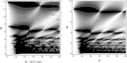
FIG. 2.: $P_{\mbox{{min }}}$as a function of the strength $E$ and energy $\hbar\omega$ of the AC field: (a) for the interacting quantum dot system ($\hbar\omega$ in units of meV) (b) for the Hubbard model with $U=8$ (both axes in units of $\tilde{t}$).

FIG. 3.: (a) Quasi-energy spectrum for the two-site model for $U=8$ and $\omega=2$, circles = exact results, lines = perturbation theory, (b) magnified view of exact results for a single anti-crossing. Beneath are the corresponding plots of $P_{\mbox{{min }}}$.

REFERENCES

- [1] M.A. Kastner, Phys. Today 46, 24 (1993); R.C. Ashoori, Nature 379, 413 (1996).
- [2] J.H. Shirley, Phys. Rev. 138, B979 (1965).
- [3] Space does not permit us to give a detailed explanation of the Floquet approach. Instead we refer the reader to the recent review article, M. Grifoni and P. Hänggi, Phys. Rep. 304, 219 (1998), for an in-depth exposition, and references within.
- [4] F. Grossmann, T. Dittrich, P.Jung and P. Hänggi, Phys. Rev. Lett. 67 516 (1991).
- [5] M. Holthaus, Z. Phys. B 59, 251 (1992).
- [6] F. Grossmann and P. Hänggi, Europhys. Lett. 18, 571 (1992).
- [7] P.I. Tamborenea and H. Metiu, Europhys. Lett. 53, 776, (2001).
- [8] R.H. Blick et al., Phys. Rev. Lett. 80, 4032 (1998).
- [9] T.H. Oosterkamp et al., Nature (London) 395, 873 (1998).
- [10] C.E. Creffield, W. Häusler, J.H. Jefferson and S. Sarkar, Phys. Rev. B 59, 10719 (1999).
- [11] H. Wang and X.-G. Zhao, J. Phys. Cond. Matt. 7, L89 (1995).
- [12] P. Zhang and X.-G. Zhao, Phys. Lett. A 271, 419 (2000).
- [13] H. Sambe, Phys. Rev. A 7, 2203 (1973).