The Local Minority Game

Abstract

Ecologists and economists try to explain collective behavior in terms of competitive systems of selfish individuals with the ability to learn from the past. Statistical physicists have been investigating models which might contribute to the understanding of the underlying mechanisms of these systems. During the last three years one intuitive model, commonly referred to as the Minority Game, has attracted broad attention. Powerful yet simple, the minority game has produced encouraging results which can explain the temporal behaviour of competitive systems. Here we switch the interest to phenomena due to a distribution of the individuals in space. For analyzing these effects we modify the Minority Game and the Local Minority Game is introduced. We study the system both numerically and analytically, using the customary techniques already developped for the ordinary Minority Game.

o

PACS: 02.50.Le; 05.40.+j; 64.60.Cn

In recent years statistical physicists have become increasingly interested in phenomena of collective behaviour related to populations of interacting individuals, typical of economic and biological systems. The aim is to find models that are easy to handle, but still describe the self organization of populations as accurately as possible. Such models can be found by applying the tools of game theory, that analyze the mechanisms of individuals reasoning in groups. Inspired by W. B. Arthur’s Farol Bar Problem [1], D. Challet and Y.-C. Zhang proposed the minority game (MG) [2]: it is a simple, but rich model describing a population of selfish individuals fighting for a common resource, as in the stock market, on roads or at waterholes. At a given time, each individual chooses between two opposing actions, that can be simplified as $a=\pm 1$. In the above examples, these options might be to buy or to sell, to take the highway or the backroad or to go to waterhole A or B. Since overall resources are limited the aim of each individual is to make the choice shared by the minority of the population. Each individual does not know what the others will choose; consequently, there is in general no best solution to the problem [3] and the individuals take their decisions using strategies, that is rules for choosing in each situation, based on the individual’s own beliefs. The only information on which an individual can base his decisions is the history $\mu$ of the game, that is the sequence of the last $M$ winning choices, e.g. $+1,+1,-1$ for $M=3$, where $M$ denotes the length of his memory. A strategy $s$ then defines which action to take in every situation, and hence consists in a sequence of $+1$s and $-1$s, one for each possible history $\mu$. Since there are two possible choices, the number of histories is $2^{M}$, which leads to a total number of $2^{2^{M}}$ possible strategies, $\{S_{i}\}$. In the original formulation of the MG, each individual was assumed to possess two strategies. These strategies are chosen by each player randomly from $\{S_{i}\}$, and never changed during the game. In general the assigned strategies differ from individual to individual: this reflects their different beliefs. Individuals do not choose a specific action, but rather a strategy that determines what action to take. At every turn of the game the strategies that would have won get a reward, and at the next turn the players choose the strategy with the highest score (this rule can be strict, or probabilistic: the strategy with the highest score has the greatest probability to be chosen). By this mechanism (reinforcement learning), players are able to learn whether they have a better strategy to use, and the system as a whole shows an extremely rich behavior.

The original MG has been studied extensively through numerical simulations, with the introduction of many different features [4], and then analytically solved through a clever mapping onto a spin glass-like model [5]. The exact solution shows that the MG undergoes a phase transition between a symmetric phase, in which all the individuals perform as if they were just acting randomly, and an asymmetric phase where some individuals always play the same strategy which turns out to be constantly the winning one. In this phase the system is the most efficient, in the sense that on the average there is always the possible maximum number of winners. Moreover, it has been shown that in the stationary state the histories may be replaced by random sequences without sensibly changing the properties of the game [6], suggesting that all the histories occur with almost the same probability (the system is almost ergodic in the history space). So far, the system has been considered as a population of individuals, each one interacting with all the others. In reality however an individual is often in contact with only a small part of the whole population. He has no information about how the members of his group interact with members of other groups, and he tries to perform optimally in his immediate surroundings.

In order to add this spatial aspect to the MG, we define a local MG (LMG) (a different local version of the MG has been introduced in  [7]). Here, every individual still has the possibility to choose one of his strategies (for simplification, a number of $S=2$ strategies is assigned to each individual) that dictates his next action. As in the global game, each individual always tries to be in the minority group by identifying the optimal strategy. The difference with respect to the MG lies in the definition of the region in which an individual is acting. In the MG every individual was interacting with all the others; in the LMG, instead, for each individual a small region is assigned, in which he attempts to be in the minority. To simplify, individuals occupy the sites of a $1d$ lattice, each one interacting with his two nearest neighbours. A region thus contains $l=3$ individuals. Each individual $i$ observes a different outcome $A_{i}$ of the game than do the others and reconstructs a different history $\mu_{i}$. His next action $a_{i}$ depends then on his own subjective local history $\mu_{i}$. The outcome $A_{i}(t)$ at time $t$ is defined as being the difference of the number of individuals that chose $a=+1$ and the number of those that chose $a=-1$. The sign of $A_{i}(t)$ then corresponds to the losing choice. Individual $i$ knows the outcome in region $i$ at time $t$, given by $A_{i}(t)=\sum_{j\in\Lambda_{i}}a_{j}^{\mu_{j}}(t)$ where $\Lambda_{i}$ denotes the set of individuals seen by player $i$. The reward for the players in the minority is then proportional to $A_{i}$ (the fewer they are, the higher the reward). The gain (or loss) individual $i$ makes at time $t$ can thus be defined as

$$u_{i}(t)=-a_{i,s_{i}}^{\mu_{i}(t)}(t)A_{i}(t),$$ (1)

where $s_{i}$ denotes the strategy he uses at time $t$, and his total profit up to $t$ is $U_{i}(t)=U_{i}(t-1)+u_{i}(t)$. The two strategies of individual $i$ are indicated with $s_{i,1}=\uparrow$ and $s_{i,2}=\downarrow$. For both his strategies individual $i$ knows the gain he would have made, if he had used that strategy. In accordance with its score, a strategy $s_{i}$ is then chosen by individual $i$ with probability

$$\pi_{i,s_{i}}(t)=\frac{e^{\beta U_{i,s_{i}}(t)}}{e^{\beta U_{i,\uparrow}(t)}+e^{\beta U_{i,\downarrow}(t)}},$$ (2)

where $\beta$ plays the role of an inverse temperature $\beta=1/T$. For a system of $N$ individuals, mean values can be written as

$$\langle A^{\mu}\rangle=\sum_{i=1}^{N}\sum_{s_{i}=\uparrow,\downarrow}\pi_{i,s_{i}}a_{i,s_{i}}^{\mu_{i}}.$$ (3)

The convention of writing $a_{i}^{\mu_{i}}=\omega_{i}^{\mu_{i}}+s_{i}\xi_{i}^{\mu_{i}}$, as it was introduced in the MG [5], leads to

$$\omega_{i}^{\mu_{i}}=\frac{a_{i,\uparrow}^{\mu_{i}}+a_{i,\downarrow}^{\mu_{i}}}{2} \xi_{i}^{\mu_{i}}=\frac{a_{i,\uparrow}^{\mu_{i}}-a_{i,\downarrow}^{\mu_{i}}}{2}.$$ and (4)

Defining $\Omega^{\mu_{i}}=\sum_{j\in\Lambda_{i}}{\omega_{j}^{\mu_{j}}}$ leads to the local outcome $A^{\mu_{i}}=\Omega^{\mu_{t}}+\sum_{j\in\Lambda_{i}}{\xi_{j}^{\mu_{j}}\,s_{j}}$. The evolution of the mean value becomes

$$m_{i}(t)=\langle s_{i}\rangle=\pi_{i,\uparrow}-\pi_{i,\downarrow}=\tanh\beta\left[U_{i,\uparrow}(t)-U_{i,\downarrow}(t)\right],$$ (5)

where for calculation we used $\uparrow=+1$ and $\downarrow=-1$. In analogy to the MG [5] the mean value is taken over all possible histories $\mu_{i}$ for each individual. Taking the time derivative of (5), and using (2), after some simple algebra the dynamics become

$$\frac{dm_{i}}{dt}=-2\beta\left[1-m_{i}^{2}\right]\frac{dH}{dm_{i}},$$ (6)

where

$$H=2\sum_{i=1}^{N}\overline{\Omega_{i}^{\mu_{i}}\xi_{i}^{\mu_{i}}}m_{i}+\sum_{i=1}^{N}\sum_{j\in\Lambda_{i}}\overline{\xi_{i}^{\mu_{i}}\xi_{j}^{\mu_{j}}}m_{i}m_{j}.$$ (7)

$\overline{O}$ denotes the mean value of a quantity $O$ over all possible histories of each region. A spin-glass hamiltonian $H=\sum_{i}h_{i}m_{i}+\sum_{i}\sum_{j\in\Lambda_{i}}J_{i,j}m_{i}m_{j}$ is thus found for spins with values $m_{i}\in\left[-1,+1\right]$ in a random field $h_{i}=\overline{\Omega_{i}^{\mu_{i}}\xi_{i}^{\mu_{i}}}$ and with random interactions $J_{i,j}=\overline{\xi_{i}^{\mu_{i}}\xi_{j}^{\mu_{j}}}$. The system minimizes $H$ for distributions $\{J_{i,j}\}$, which are given by the initial distribution of strategies among the individuals.

In the intuitive example of two anticorrelated strategies per individual, the action performed by strategy $\uparrow$ of individual $i$ is the opposite of the action performed by his strategy $\downarrow$ for every history, i.e. $a_{i,\uparrow}^{\mu_{i}}=-a_{i,\downarrow}^{\mu_{i}}$. As a result, $\omega_{i}^{\mu_{i}}=0\;\forall\;i,\mu_{i}$ and thus the field $h_{i}$ vanishes. In the simple case of $M=1$ the system behaves like an antiferromagnet. This is straightforward, since the best configurations are individuals taking alternative actions ($\uparrow\downarrow\uparrow\downarrow\uparrow$ etc.). For $M=1$, chosing a strategy is equivalent to choosing an action. For periodic boundary conditions and an even number $N$ of individuals, everyone wins. Analytically this can be understood by calculating $J_{i,j}=\overline{\xi_{i}^{\mu_{i}}\xi_{j}^{\mu_{j}}}$. On the one hand $\overline{\xi_{i}^{\mu_{i}}\xi_{j}^{\mu_{j}}}=1\;\forall\;i,j$ for which $a_{i,\uparrow}^{\mu_{i}}=a_{j,\uparrow}^{\mu_{j}}$ and on the other hand $\overline{\xi_{i}^{\mu_{i}}\xi_{j}^{\mu_{j}}}=-1\;\forall\;i,j$ for which $a_{i,\uparrow}^{\mu_{i}}=a_{j,\downarrow}^{\mu_{j}}$, independent of the history. This corresponds to an antiferromagnetic spin system at $T=0$. The individuals build clusters in which everyone is frozen to one of his strategies and therefore constantly wins. Between two incompatible clusters there is a boundary on which individuals are frustrated. Unlike the MG where the maximum number of winners is $(N-1)/2$, the LMG shows configurations where every individual can win, depending on the nature of the regions. For increasing $M$ the number of frozen individuals decreases until the system reaches the state of random individuals, a behavior which is confirmed by simulations. This example shows clearly how the LMG differs from the MG. In the MG, the case of two anticorrelated strategies is inefficient, which can be clearly understood since it corresponds to an antiferromagnet in infinite dimensions, while in the LMG it can lead to situations where everyone wins.

The LMG is generalized to two dimensions by placing the individuals on a square lattice with periodic boundary conditions. Now each individual has four nearest neighbours and the regions are chosen to consist of $l=5$ individuals. Strategies are still taken as anticorrelated, thus implying a vanishing random field $\{h_{i}\}$. Analogous to the one-dimensional case, a mapping on a spin system can be performed, which leads to the partition function

$$Z[\{J_{i,j}\}]=\int_{-1}^{+1}{\prod_{i}dm_{i}e^{-\beta H[\{J_{i,j},m_{i},m_{j}\}]}}.$$ (8)

In order to calculate the free energy, the average over the distribution of the interactions $\{J_{i,j}\}$ needs to be taken. Still we do not know whether we should take the average of the partition function itself (8) or of the free energy. The choice depends on whether in (7) the interactions are annealed or quenched random variables. Numerical simulations determine the distributions $P\left(J_{i,j}\right)$ to be nearly gaussian at high temperatures, where the system is disordered ($m\simeq 0$; players randomly switch between their strategies) and bimodal at low temperatures, where almost all players are frozen ($|m|\simeq 1$; each player always plays the same stategy). In the latter case $J_{i,j}=\pm 1$. Since both the spins and the distribution of the interactions change during the dynamics, the disorder is annealed, at variance with the ordinary MG, where disorder is quenched. The origin of this behavior is in the dynamics in history space: whereas the MG is (quasi)ergodic, so that the averages in (7) do not change in time, the players of the LMG in the stationary state see just one single history, and ergodicity is broken. Moreover they always choose a strategy that allows them to be in the minority of their local environemnt, which leads to an effective aniferromagnet. Temperature is not the only parameter affecting the distribution $P\left(J_{i,j}\right)$: increasing $M$, a sudden change from a bimodal to a gaussian distribution takes place (see Fig.1).

Actually, the dependence of the state of the system and of the distribution of the interactions on $T$ and $M$ is not accidental. The $\{m_{i}\}$ as well as the interactions $\{J_{i,j}\}$ are free to take values which minimize the Hamiltonian $H[\{J_{i,j},m_{i},m_{j}\}]$ of the system, which therefore is identified as an annealed system with the partition function

$$Z_{\rm{ann}}=\int_{-\infty}^{+\infty}\prod_{i,j\in\Lambda_{i}}dJ_{i,j}P[J_{i,j}]\int_{-1}^{+1}{\prod_{i}dm_{i}e^{-\beta H[\{J_{i,j},m_{i},m_{j}\}]}}.$$ (9)

Before thermalization (i.e. before the dynamics), the distribution $P\left(J_{i,j}\right)$ is nearly gaussian (implying that all histories are equiprobable),

$$P(J_{i,j})=\frac{1}{\sqrt{2\pi}\sigma_{J}}e^{-\frac{J_{i,j}^{2}}{2\sigma_{J}}}\;\;.$$ (10)

As a consequence, the hamiltonian of the system can be written as

$$H_{\rm{ann}}[\{J_{i,j},m_{i},m_{j}\}]=\sum_{i=1}^{N}\sum_{j\in\Lambda_{i}}\left(\frac{J_{i,j}^{2}}{2\beta\sigma_{J}^{2}}-J_{i,j},m_{i},m_{j}\right).$$ (11)

After an integration over the disorder the partition function becomes

$$Z_{\rm{ann}} = \int_{-1}^{+1}{\prod_{i}dm_{i}e^{\frac{\beta^{2}\sigma_{J}^{2}}{2}\sum_{i,j\in\Lambda_{i}}{m_{i}^{2}m_{j}^{2}}}}$$ (12)

$$= \int_{-1}^{+1}{\prod_{i}dm_{i}e^{-\tilde{\beta}H_{eff}}}$$

where $\tilde{\beta}\equiv\frac{\beta^{2}\sigma_{J}^{2}}{2}$ and $H_{eff}=-\sum_{i,j\in\Lambda_{i}}m_{i}^{2}m_{j}^{2}$ is the effective hamiltonian, which no longer depends explicitly on $\{J_{i,j}\}$.

At low temperatures the system tends to $<m_{i}^{2}>=1$, while at high temperatures $<m_{i}^{2}>=\int_{-1}^{+1}\frac{m_{i}^{2}}{2}dm_{i}=\frac{1}{3}$, because in this case all possible values of $m_{i}$ occur with uniform probability in $[-1,+1]$. In between, a critical temperature $\tilde{T}_{c}$ is observed, which separates the two cases, and obeys $T_{c}^{2}\propto\tilde{T}_{c}\sigma_{J}^{2}$. An approximative calculation of the variance $\sigma_{J}^{2}=<J_{I,j}^{2}>$ depending on $M$ confirms a phase boundary at $T_{c}\sim\sigma_{J}\sim 2^{-M}$. This last result can be obtained assuming that the histories of the neighbors $i$ and $j$ are independent (which of course is an approximation). Fig.1 shows the distribution $P[\{J_{i,j}\}]$ in the stationary phase for three values of $M$ at a given temperature $T=1.0$. As can be seen, there is a sharp transition from a bimodal distribution for $M=2$ and $M=3$ to a nearly gaussian distribution for $M=4$. In Fig.2 the stationary state of the system for $M=3$ and $T=1.0$ is represented, clearly showing that the system is ordered (white squares represent frozen players, black squares unfrozen ones), with a bimodal distribution of the interactions. For small values of $M$, all the individuals always use only one of their strategies and win. The histories therefore do not change over time, which clearly breaks the ergodicity of the dynamics in history space. For $M=4$, however, the system is in the disorderd phase and all the histories occur with roughly the same probability. This confirms the calculated phase transition at a critical temperature $T_{c}$ which is proportional to $\sigma_{J}\propto\frac{1}{2^{M}}$. At higher temperature, the phase transition from the bimodal to the gaussian distribution takes place at lower values of $M$. The phase diagram is displayed in Fig.3.

In the case of small regions, as considered in the above calculations, the influence of the individual agents on the outcome cannot be neglected; indeed, if one agent had chosen his unused strategy in the last step, the winning choice could have easily been the other one. When an agent does not know the effective impact of both his strategies in the last step, but only the outcome while using one of them, he overestimates his second, unused strategy considerably [8]. A clearly higher efficiency is thus observed in a population with complete information, meaning the agents know about the influence that both their strategies have on the outcome. In such a system nearly all the agents win at low temperature and only at very high temperature and for large $M$ does decreasing efficiency occur. Even for $T=1000$ and $M=8$ the system is clearly in the ordered phase with $99.9\%$ of all the individuals frozen to one of their strategies. If the histories are replaced by random sequences of winning choices, the system with complete information is still more efficient than the one with partial information, but not as clearly as for real histories. The case of partial information, however, is the most realistic.

Although the basic principles of the LMG are the same as for the MG, the behaviors of the two systems have considerable differences in important features. Unlike in the MG, where all the individuals interact with each other, the interactions in the LMG are only local. The system nevertheless shows a global, collective behavior, because it benefits from the spatial arrangement of the individuals. The dynamics minimize a hamiltonian that still depends on the $m_{i}$, as in the MG. Yet in the LMG also the interactions change during the dynamics: the disorder is annealed, while in the MG it is quenched. Whereas the case of two anticorrelated strategies per individual is inefficient in the MG, in the LMG it is highly efficient and there are cases where all the individuals can win. On the other hand, random strategies are disadvantageous in the LMG, because here every individual has his own, subjective information. In a magnetic system language, random strategies are in general incompatible with $J_{i,j}=\pm 1$, that is the best interaction in the ordered case, and some residual disorder will still be present even at low temperatures. Moreover, random strategies give rise to a non-vanishing random fields $h_{i}$. In two-dimensionsit is known that the random-field Ising model is disordered down to $T=0$. Hence, we would need a three dimensional system to recover the phase transition described above.

Our analysis has therefore shown, analytically and numerically, that despite their similar structure, the MG and the LMG are significantly different: whereas in the MG players organize in time, in the LMG space correlations become important. It is concievable that reality sits in between these two extreme cases: players could gather information both from their local environments and from some distant sources: a small-world type of connections could be a good modelization ofsuch a scenario; alternatively, histories could be formed mixing both the local and the global information, with weigths mimicking the relevance of each of them to the players. It is appealing to think that both time and space coordinations could become important in such mixed games.

The authors thank the University of Fribourg (CH), where this work was begun. This work has been supported by the Swiss National Science Foundation under contract FNRS 21-61397.00 and by the EU Network ERBFMRXCT980183. A Java Applet to play with the LMG can be found at
http://www.unifr.ch/perso/moelbert/lmg_nn_fro/lmg_nn_hole_not_fro.html

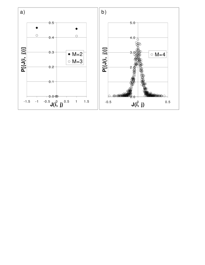
Figure 1: Distribution $P[\{J_{i,j}\}]$ at temperature $T=1.0$ for the two dimensional LMG with nearest neighbor interaction and anticorrelated strategies. a) For $M=2,3$ the system is in the ordered phase, b) while for $M=4$ it is in the disordered phase.

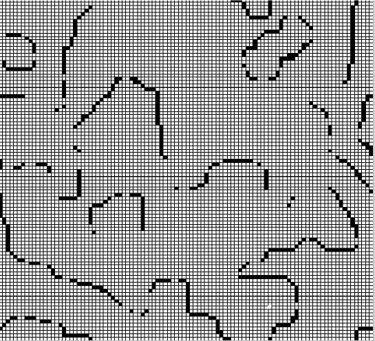
Figure 2: The system for $M=3$ and $T=1.$: white squares correspond to frozen players, black squares to players that have not yet frozen.

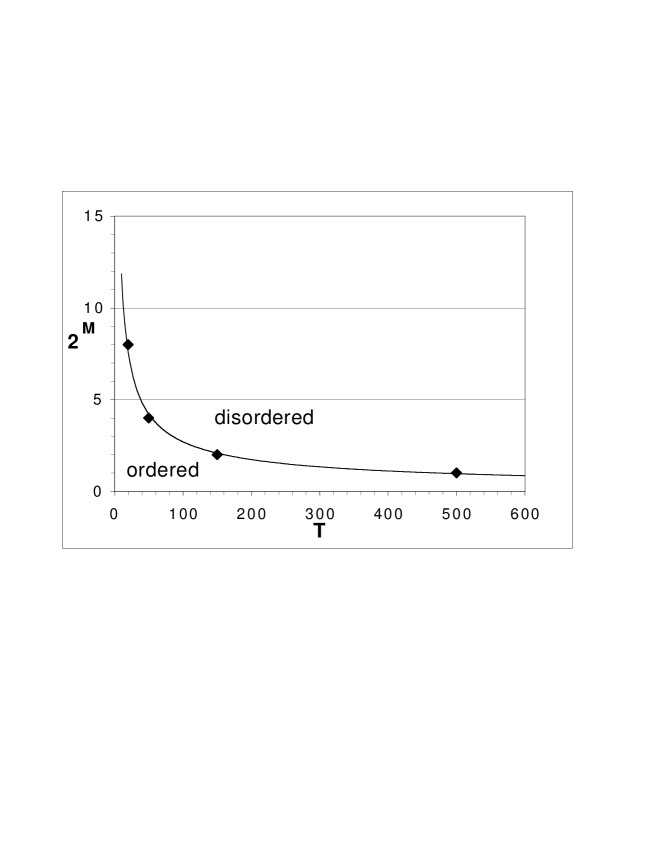
Figure 3: Phase diagram for the LMG with anticorrelated strategies in two dimensions, where each individual interacts with his four nearest neighbors. The system is in the ordered phase for low temperatures and low $M$.

References

- [1] W.B. Arthur, Amer. Econ. Assoc. Papers and Proc. 84, 406 (1994).
- [2] D. Challet and Y.-C. Zhang, Physica A 246, 407 (1997).
- [3] D. Fudenberg and J. Tirole, Game Theory, (MIT Press, Cambridge, 1993); J. W. Weibull, Evolutionary Game Theory, (MIT Press, Cambridge, 1995).
- [4] D. Challet and Y.-C. Zhang, Physica A 256, 514 (1998); R. Savit, R. Manuca and R. Riolo, Phys. Rev. Lett. 82, 2203 (1999). N.F. Johnson, M. Hart and P.M. Hui, Physica A, 269, 1 (1999); R. D’hulst and G.J. Rodgers, Physica A, 270, 222 (1999).
- [5] D. Challet and M. Marsili, Phys. Rev. E 60, R6271 (1999); D. Challet, M. Marsili and R. Zecchina, Phys. Rev. Lett. 84, 1824 (2000); M. Marsili, D. Challet and R. Zecchina, Physica A 280, 522 (2000).
- [6] A. Cavagna, Phys. Rev. E 59, R3783 (1999).
- [7] T. Kalinowski, H.-J. Schultz and M. Briese, Physica A 277, 502 (2000).
- [8] D. Challet and M. Marsili, Phys. Rev. E 60, R6271 (1999).
- [9] M. Mézard, G. Parisi and M. A. Virasoro, Spin Glass Theory And Beyond (World Scientific, Singapore, 1986).