Magneto-localization in Disordered Quantum Wires

Abstract

The magnetic field dependent localization in a disordered quantum wire is considered nonperturbatively. An increase of an averaged localization length with the magnetic field is found, saturating at twice its value without magnetic field. The crossover behavior is shown to be governed both in the weak and strong localization regime by the magnetic diffusion length $L_{B}$. This function is derived analytically in closed form as a function of the ratio of the mean free path $l$, the wire thickness $W$, and the magnetic length $l_{B}$ for a two-dimensional wire with specular boundary conditions, as well as for a parabolic wire. The applicability of the analytical formulas to resistance measurements in the strong localization regime is discussed. A comparison with recent experimental results is included.

Contents

toc

I INTRODUCTION

The phase coherent movement of electrons in a disorder potential can result in strong localization due to quantum interference [1, 2]. As soon as the localization length $L_{c}$ becomes smaller than the size of the sample $L$ and the phase coherence length, $L_{\phi}$, the resistance increases exponentially.

The strong localization due to quantum interference is known to depend on the global symmetry of the disordered electron system [3]. In disordered quantum wires, the localization length is

$$L_{c}=\beta\pi\hbar\nu SD_{0},$$ (1)

where $\beta=1,2,4$, corresponding to no magnetic field, finite magnetic field, and strong spin- orbit scattering or magnetic impurities, respectively. $\nu(E)$ is the electronic density of states in the wire. $D_{0}=\tau v_{F}^{2}/d$ is the classical diffusion constant of the electrons in the wire, with $\tau$ the elastic scattering time, $v_{F}$ the Fermi velocity, and $d$ the dimension of classical diffusion. $S$ is the wire crossection. This result was first obtained by calculating the spatial decay of the density correlation function for wires with diffuse crossections and many transversal channels $N\gg 1$. It can also be obtained by calculating the transmission probability through thin, few channel wires upto a correction of order $1/N$: $L_{c}=(\beta N+2-\beta)l$ [1], where $l=v_{F}\tau$ is the mean free path, and $\beta=1,2,4$, as defined above. This correction ensures that the localization length is for a single channel, $N=1$, independent of $\beta$, $L_{c}=2l$.

Recently, the doubling of the localization length was observed in sub-micron thin wires of Si $\delta$- doped Ga As structures by Khavin, Gershenson and Bogdanov, who found a continously decreasing activation energy when the magnetic field is increased, saturating indeed at one half of its field free value [4]. This symmetry dependence of the localization properties of quantum wires allows to test our present theoretical understanding by detailed comparison with the experiment. The quantum wires used in the experiment have mean free paths which are smaller than or comparable to their thickness. Also, in addition to the disorder in the bulk due to the random electrostatic potential of the donor impurities, there is an unspecified surface roughness which may influence the classical mobility of the wires as well as its quantum transport properties. Therefore, a more detailed analysis of the localization length as function of these parameters is called for, in order to be able to compare the theory with the experimental results quantitatively.

In the next section we review the known weak localization corrections to the conductivity in disordered quantum wires and their magneto-sensitivity as function of mobility, wire thickness, and electron density [5, 6, 7, 8].

In the third section, the non-perturbative theory of localization in disordered electron systems[2] is extended, in order to allow the study of wires with ballistic crossections.

In the fourth section, the magnetic phase shifting rate is introduced and identified with a correlation function of the magnetic vector potential, relating it to the coefficient of the time reversal symmetry breaking term in the nonlinear sigma model. This expression for the magnetic phase shifting rate, is calculated anayltically for arbitrary ratios of the mean free path $l$ and the width of the wire $W$, and compared with previously derived analytical and numerical results[6, 8] for a wire with specular boundary scattering.

Next, it is calculated for a wire with harmonic confinement which allows to extend the analysis to stronger magnetic fields, when the cyclotron radius, $l_{\rm C}$ is smaller than the the wire thickness $W$, but still larger than the elastic mean free path. In that regime a new enhancement mechanism for the magnetic phase shifting rate leading to a stronger magneto-sensitivity, is identified.

In the fifth section, the autocorrelation function of spectral determinants (ASD)[9, 10] is considered for a coherent disordered quantum wire, which shows the expected crossover from Wigner- Dyson statistics[11], typical for a spectrum of extended states in phase coherent disordered metal systems[2], to Poisson statistics, corresponding to a spectrum of localized states [12, 13, 14, 15, 16, 17], as the length of the wire is increased beyond a localization length $L_{C}$, as reported earlier[18].

This crossover length scale to Possionian statistics is used to derive the averaged localization length of disordered quantum wires, and it is shown that it yields the correct symmetry dependence, Eq. (1). A comparison with the result of the supersymmetric theory of the two-terminal conductance of a disordered quantum wire, is given. It is concluded, that the definition of an averaged localization length, by the decay of an energy level correlation function, can be used to consider analytically the magnetic field dependence of the localization length. Thereby, analytical formulas for the localization length as a function of wire width, mean free path and magnetic field are derived.

In the sixth section, the theory of finite tempreature magnetoresistance in quantum wires is discussed. In particular, the variable range hopping conductivity in quantum wires is reviewed for various temperature and dimensional regimes. It is shown that in a wide temperature regime the resistance has an activated behaviour, and that therefore, the activation gap can be directly measured and related to the localization length of the electrons in the wire.

This allows a comparison of the analytical results for the magnetic field dependence of the localization length with these experimental results, as done in the seventh section.

In appendix A, the functional integral representation of the ASD by Grassmann intergals is given, and the averaging over disorder is performed. In appendix B the derivation of the magnetic phase shifting rate is given. In appendic C the representation of the matrix fields $Q$ is given, and their Laplacian derived.

II Weak Localization

Classically, the transport of a disordered conductor is characterized by its mobility $\mu=q\tau/m$ and the electron density $n$ related to the the classical Drude conductivity $\sigma_{0}=nq^{2}\tau/m$. Alternatively, it can be characterized by the diffusion constant $D$, which is in a metal related to the conductivity by the Einstein relation $\sigma_{0}=2q^{2}\nu D$.

When the electrons diffuse coherently, quantum interference without magnetic field results in a suppression of the conductivity of a quantum wire of order[1, 19, 20, 21, 22, 23]

$$\frac{\Delta\sigma}{\sigma_{0}}=-\frac{2}{\sqrt{2\pi^{3}}}(\frac{\sqrt{\tau_{\varphi}}}{\sqrt{\tau}}-1),$$ (2)

where $\tau_{\phi}$ is the phase coherence time, that increases when decreasing the temperature as a power law:

$$\tau_{\phi}\sim T^{-\gamma}$$ (3)

and defines the phase coherence length, which an electron diffuses coherently, $L_{\phi}=(D\tau_{\phi})^{1/2}$.

Quasi elastic electron-electron scattering can be the dominant low temperature dephasing mechanism and yields $\gamma=2/3$ for a 1-d wire and $\gamma=1$ for a 2-d film [7, 24]. At higher temperatures the exponent crosses over to $\gamma=4$ due to electron-phonon scattering at temperatures $k_{\rm B}T\ll(\hbar^{2}/\tau\epsilon_{F})\Omega_{D}$ where $\Omega_{D}$ is the optical Debye phonon frequency. This power can be smaller, due to the confinement, in quantum wires.

The above definition of the phase coherence rate is not applicable when approaching the localized regime, and the phase coherence length is larger than the localization length $L_{c}$. Also, there are mechanisms which may lead to a saturation of $\tau_{\phi}$ below $T=1K$, as observed in a wide range of conductors [25, 26].

A magnetic field breaks the time reversal symmetry. Therefore, the magnetic phase accumulated in a Brownian motion of electrons, enters effectively as an additive contribution to the phase coherence rate, diminishing the weak localization corrections of the conductivity[21]. For wires with diffusive width $W>l$, it varies quadratically with the magnetic field, $1/\tau_{\phi}(B)=1/\tau_{\phi}+D\frac{q^{2}}{\hbar^{2}}SB^{2}/K_{D}$, where S is the crossection of the wire, and the constant $K_{D}$ depends on the geometry of the wire, the direction of the magnetic field and the scattering mechanisms [5]. For example, for a 2-dimensional wire of diffusive crossection in a perpendicular magnetic field, it yields, $K_{D}=3$. In this way, the conductivity increases to its classical value, when the magnetic field is turned on.

For a wire with ballistic crossection and a magnetic field being perpendicular to its crossection, the magnetic field dependence of the weak localization correction to the conductivity is weakened by flux cancellation effects due to boundary scattering[6]. If the magnetic field is so small that less than one flux quantum $\phi_{0}=h/e$ is penetrating an area $Wl$, the effective dephasing rate $1/\tau_{\phi}(B)$ is quadratically increasing as for diffusive crossections. Its slope was found to be by at least a factor $W/l$ smaller, as a consequence of the flux cancellation effect of edge to edge skipping orbits[6, 8].

When $BWl\gg\phi_{0}$, the effective dephasing rate $1/\tau_{\phi}(B)$ was found by a semiclassical method, to increase only linearly with the magnetic field $B$ in this regime[6, 8].

In the presence of magnetic impurities, scattering the electrons with a rate $1/\tau_{S}$, there is no temperature dependence of the conductivity, if $1/\tau_{S}\gg 1/\tau_{\phi}$.

Strong spin-orbit scattering reverses the sign of the quantum correction to the conductivity[27]. The conductivity is then larger than classically expected. This can be observed by increasing an external magnetic field, which destroys time reversal invariance and acts through an effective decoherence time $1/\tau_{\phi}(B)=1/\tau_{\phi}$ as noted above. In the case of moderately strong spin-orbit scattering, the conductivity decreases therefore when the magnetic field is turned on[7].

At low temperatures, when the dephasing rate $1/\tau_{\phi}$ becomes smaller than the typical energy scale of strong localization, the local level spacing $\Delta_{C}=1/(\nu WL_{C})$, a perturbation theory in the elastic scattering rate $1/\tau$ is no longer appropriate, and a nonperturbative treatment of disorder is called for, as the scaling theory of localization does indicate[19, 20].

III Nonperturbative theory of localization in disordered quantum wires

In this section, the nonperturbative theory of disordered noninteracting electrons in quantum wires is derived[28, 22, 2]. Its action, governed by the long wave length modes corresponding to diffusion, the nonlinear sigma model is rederived, extending previous derivations, to allow the description of quantum wires with ballistic crossections.

The Hamiltonian of disordered noninteracting electrons is

$$H=\epsilon\left({\bf p}-q{\bf A}\right)+V({\bf x})+{\bf\sigma b_{s}(x)}+{\bf\sigma u_{SO}}\times{\bf p},$$ (4)

where $q$ is the electron charge. In the following, we will generally approximate the electronic dispersion $\epsilon\left({\bf p}-q{\bf A}\right)$ by $\left({\bf p}-q{\bf A}\right)^{2}/(2m)$, where $m$ is the effective electron mass, but note that higher moments are sometimes needed to regularize the correlation functions, calculated below.

$V({\bf x})$ is taken to be a Gaussian distributed random function $\left<V({\bf x})\right>=0$, and $\left<V({\bf x})V({\bf x^{\prime}})\right>=\hbar\Delta SL/(2\pi\tau)\delta({\bf x}-{\bf x^{\prime}}),$ which models randomly distributed, uncorrelated impurities in the sample. $\Delta=1/(\nu SL)$ is the mean level spacing. This corresponds to a Gaussian distribution function $P(V)=\exp(-\frac{\pi\tau}{\hbar\Delta}\int\frac{d{\bf x}}{Vol.}V({\bf x})^{2})$ of the disorder potential, defining the disorder average as $<...>_{V}=\int\prod_{{\bf x}}dVP(V)...$. According to the central limit theorem, this is therefore a good description of the various sources of randomness in the electrostatic potential, in which the electrons are moving.

The vector potential is used in the gauge ${\bf A}=(-By,0,0)$, where $x$ is the coordinate along the wire of length L, $y$ the one in the direction perpendicular both to the wire and the magnetic field ${\bf B}$, which is directed perpendicular to the wire. The angular brackets denote averaging over impurities. ${\bf\sigma}$ is the electronic spin operator, and ${\bf b_{s}(x)}$ is a random magnetic impurity field. ${\bf u_{SO}}$ is the local electrostatic field of impurities with large atomic number $Z$, which do give a stronger spin orbit coupling to the conduction electrons.

The Hamiltonian can be classified by its symmetry with respect to time reversal and spin rotation as summarized in Table 1.

It has been noted that the averaged density of states or the averaged one-particle Green’s function does not contain any information on the localization of Eigenfunctions of the disordered Hamiltonian $H$[28]. The physical reason is, that the one-particle Green’s function describes the propagation of the wave function amplitude $\psi({\bf x})$. Elastic impurity scattering randomizes the phase of the amplitude and therefore, this propagator decays on the scale of the mean free scattering time $\tau$. To catch classical diffusion and quantum localization, at least the evolution of the density or amplitude square has to be averaged over the disorder, leading to a correlation function of two one-particle Green’s functions. While weak localization corrections can be calculated within a diagrammatic perturbation expansion of such correalation functions [5, 23], the study of strong electron localization in a disordered potential, necessitates a nonperturbative averaging of such products of Green’s functions. This can be achieved by means of the super-symmetry method, whereby the product of Green’s functions is written as a functional integral[2]. Thus, the average over the form of the disorder potential can be done right at the beginning as a Gaussian integral, exactly.

Here, for simplicity, we present the derivation of a simpler correlation function, which does not necessitate the use of the full super-symmetry method, but still contains some information on strong quantum localization, as shown recently[18, 29, 30].

The statistics of discrete energy levels of a finite coherent, disordered metal particle is an efficient way to characterize its properties [2]. This can be studied by calculating a disorder averaged autocorrelation function between two energies at a distance $\omega$ in the energy level spectrum. Thereby, an uncorrelated spectrum of localized states can be distinguished from a correlated spectrum of extended states.

The autocorrelation function of spectral determinants (ASD) is the most simple such spectral correlation function, which allows to explore complex quantum systems analytically, and still does contain nontrivial information on level statistics and, thus, on localization[18, 29].

It is an oscillatory function whose amplitude decays with a power law, when the energy levels in the vicinity of the central energy $E$ are extended, while a Gaussian decay is a strong indication that all states are localized.

It is defined by $C(\omega)=\bar{C}(\omega)/\bar{C}(0),\hskip 14.22636pt\bar{C}(\omega)=\left<\mbox{det}(E+\omega/2-H)\mbox{det}(E-\omega/2-H)\right>,$ where $E$ is a central energy.

Since it is a product of two spectral determinants, and a spectral determinant can be written as a Gaussian functional integral over Grassmann variables $\psi$, $\psi^{*}$, one does need at least a 2-component Grassman field, one for each spectral determinant.

In general, $4\alpha$ -component Grassman fields are needed to get the functional integral representation of the ASD. Here, $\alpha=1$, when the Hamiltonian is independent of the spin of the electrons, and each level is doubly spin degenerate. There is one pair of Grassman fields for each determinant in the ASD and each pair is composed of a Grassman field and its time reversed one, as obtained by complex conjugation. $\alpha=2$ has to be considered, when the Hamiltonian does depend on spin, as for the case with moderately strong magnetic impurity or spin- orbit scattering. This necessitates the use of a vector of a spinor and the corresponding time reversed one.

The representation as a Gaussian functional integral over Grassmann variables is given explicitly for $\alpha=1$ in appendix A. There, the averaging over disorder and the decoupling of the resulting $\psi^{4}$ interaction with a Gaussian integral over a matrix field $Q$ is given. Thus, the disorder averaged ASD is given by a functional integral over a matrix field $Q$.

The matrix $Q$ is element of the full symmetric space, including rotations between the subspace corresponding to the left and the right spectral determinant. Therefore, the long wavelength modes of $Q$, do contain the nonperturbative information on the diffuson and Cooperon modes.

In order to consider the action of long wavelength modes governing the physics of diffusion and localization, one can now expand around the saddle point solution of the action, satisfying for $\omega=0$,

$$Q=i/(\pi\nu)<{\bf x}\mid 1/(E-H_{0}+i\hbar/(2\tau)Q)\mid{\bf x}>.$$ (5)

This saddle point equation is found to be solved by $Q_{0}=\Lambda$. For $\alpha=1$, and $B=0$, at $\omega=0$, the rotations $U$, which leave $Q$ in the symplectic symmetric space yield the complete manifold of saddle point solutions as $Q=\bar{U}\Lambda U$, where $U\bar{U}=1$, with $Q^{T}C=CQ$. The modes which leave $\Lambda$ invariant, elements of $Sp(1)\times Sp(1)$ are surplus, or spontanously broken, and can be factorized out, leaving the saddle point solutions to be elements of the symmetric space $Sp(2)/(Sp(1)\times Sp(1))$[31].

For $\alpha=2$ the matrix $C$ is, due to the time reversal of the spinor, substituted by $i\sigma_{2}\tau_{1}$[22]. Both magnetic impurities and spin-orbit scattering reduce the Q matrix to unity in spin space. Thus, C has effectively the form $\tau_{1}$. The condition $Q^{T}C=CQ$ leads therefore to a new symmetry class, when the spin symmetry is broken but the time reversal symmetry remains intact. This is the case for moderately strong spin-orbit scattering. Then, $Q$ are $4\times 4$- matrices on the orthogonal symmetric space $O(4)/(O(2)\times O(2))$ [28], which is the nonperturbative consequence of the sign change of a spinor component under time reversal operation, which leads to the positive quantum correction to the conductivity in perturbation theory [23]. With magnetic impurities both the spin and time reversal symmetry is broken, and the Q- matrices are in the unitary symmetric space $U(2)/(U(1)\times U(1))$ as for a moderate magnetic field and spin degenerate levels. The difference in the prefactor $\alpha$ remains. One can extend this approach to other compact symmetric spaces with physical realizations, see Ref. [32, 33] for a complete classification.

In addition to these gapless transversal modes there are massive longitudinal modes with $Q^{2}\neq 1$, which for $N\gg 1$, can be integrated out[2], and the ASD thereby reduces to a functional integral over the transverse modes $U$. Now, the action of finite frequency $\omega$ and spatial fluctuations of $Q$ around the saddle point solution can be found by an expansion of the action $F$, Eq. (75). Inserting $Q=\bar{U}\Lambda U$ into Eq. (75), and performing the cyclic permutation of $U$ under the trace $Tr$, yields,

$$F=-\frac{1}{2}\int d{\bf x}<{\bf x}\mid Tr\ln(G_{0}^{-1}-U[H_{0},\bar{U}]+\omega U\Lambda\bar{U})\mid{\bf x}>,$$ (6)

where

$$G_{0}^{-1}=E-H_{0}+\frac{i\hbar}{2\tau}\Lambda.$$ (7)

Expansion to first order in the energy difference $\omega$ and to second order in the commutator $U[H_{0},\bar{U}]$, yields,

$$F[U] = -\frac{1}{2}\omega\int d{\bf x}<{\bf x}\mid TrG_{0E}U\Lambda\bar{U}\mid{\bf x}>$$ (8)

$$+ \frac{1}{2}\int d{\bf x}<{\bf x}\mid TrG_{0E}U[H_{0},\bar{U}]\mid{\bf x}>$$ (9)

$$+ \frac{1}{4}\int d{\bf x}<{\bf x}\mid Tr(G_{0E}U[H_{0},\bar{U}])^{2}\mid{\bf x}>.$$ (10)

Note that $[H_{0},\bar{U}]=-\frac{\hbar^{2}}{2m}({\bf\nabla}^{2}\bar{U})-\frac{\hbar^{2}}{m}({\bf\nabla}\bar{U}){\bf\nabla}-\frac{q\hbar}{imc}(\tau_{3}{\bf A}{\bf\nabla}\bar{U}-\bar{U}\tau_{3}{\bf A}{\bf\nabla})$.

The first order term in $U[H_{0},\bar{U}]$ vanishes for Gaussian white noise isotropic scattering.

In general, in order to account for the ballistic motion of electrons in ballistic wires, or to account for different sources of randomness, a directional dependence of the matric $U=U({\bf x}.{\bf n})$, where ${\bf n}={\bf p}/\mid{\bf p}\mid$, has to be considered[34, 35]. However, for the geometries considered in this article, we have found that the form of the action derived below remains valid for diffusive as well as ballistic crossections, when the vector fields ${\bf S}$ as intorduced in Refs. [34, 35], are integrated out. This will be presented in more detail in a separate article.

Then, one can keep second order terms in ${\bf\nabla}\bar{U}$ and ${\bf A}$, which turns out to be valid for the regime of weak disorder, $l\gg 1/k_{F}$ and for any magnetic field, $l_{B}\gg k_{F}$. Thus, one gets, using the saddle point equation, Eq. (5),

$$F[U] = -\frac{\pi}{4}\frac{\omega}{\Delta}\int\frac{d{\bf x}}{SL}Tr\Lambda Q$$ (11)

$$+ \frac{1}{4}\int d{\bf x}<{\bf x}\mid Tr(G_{0E}U(\frac{\hbar^{2}}{2m}({\bf\nabla}\bar{U})({\bf\nabla}-\frac{i}{\hbar}q{\bf A}\tau_{3})+\frac{q\hbar}{m}[\tau_{3},\bar{U}{\bf A}{\bf\nabla}]))^{2}\mid{\bf x}>.$$ (12)

Next, one can separate the physics on different length scales, noting that the physics of diffusion and localization is governed by spatial variations of $U$ on length scales larger than the mean free path $l$. The smaller length scale physics, is then included in the correlation function of Green’s functions, being related to the conductivity by the Kubo-Greenwood formula,

$$\sigma_{\alpha\beta}(\omega)=\frac{\hbar}{\pi SL}\frac{q^{2}}{m^{2}}\sum_{\bf p,p^{\prime}}(p_{\alpha}-qA_{\alpha})(p^{\prime}_{\beta}-qA_{\beta})<{\bf p}\mid G^{R}_{0E}\mid{\bf p^{\prime}}><{\bf p^{\prime}}\mid G^{A}_{0E+\omega}\mid{\bf p}>,$$ (13)

where ${\bf p}=\frac{\hbar}{i}{\bf\nabla}$. The remaining averaged correlators, involve products $G^{R}_{0E}G^{R}_{0E+\omega}$ and $G^{A}_{0E}G^{A}_{0E+\omega}$ and are therefore by a factor $\hbar/(\tau E)$ smaller than the conductivity, and can be disregarded for small disorder $\hbar/\tau\ll E$. In the bulk of this article we are interested in the weak magnetic field limit, where $\omega_{c}\tau\ll 1$, with the cyclotron frequency $\omega_{c}=qB/m$. In this limit we can disregard the nondiagonal Hall conductivity and the explicit magnetic field dependence of the longitudinal conductivity.

In order to insert the Kubo-Greenwood formula in the saddle point expansion of the nonlinear sigma model, it is convenient to rewrite the propagator in $F$ as $G_{0E}=\frac{1}{2}G^{R}_{0E}(1+\Lambda)+\frac{1}{2}G^{A}_{0E}(1-\Lambda)$.

Then, we can use, that $Tr[\sum_{\alpha=1}^{d}\sum_{s=\pm}(1+s\Lambda)U(\nabla_{\alpha}\bar{U})(1-s\Lambda)U(\nabla_{\alpha}\bar{U})]=-Tr[({\bf\nabla}Q)^{2}]$, and $Tr[\sum_{s=\pm}(1+s\Lambda)U[\tau_{3},\bar{U}]](1-s\Lambda)U[\tau_{3},\bar{U}]=-Tr[[\tau_{3},Q]^{2}]$.

Thereby we can rewrite Eq. (11) as

$$F[Q] = -\frac{\pi}{4}\frac{\omega}{\Delta}\int\frac{d{\bf x}}{SL}Tr\Lambda Q$$ (14)

$$- \frac{1}{4}\int d{\bf x}Tr[({\bf\nabla}Q({\bf x}))^{2}<{\bf x}\mid G_{0E}^{R}\frac{\hbar^{2}}{2m}({\bf\nabla}-\frac{i}{\hbar}q{\bf A})G_{0E}^{A}\frac{\hbar^{2}}{2m}({\bf\nabla}-\frac{i}{\hbar}q{\bf A})\mid{\bf x}>$$ (15)

$$- \frac{1}{4}(\frac{q\hbar}{m})^{2}\int d{\bf x}Tr[[\tau_{3},Q({\bf x})]^{2}]<{\bf x}\mid G_{0E}^{R}{\bf A}{\bf\nabla}G_{0E}^{A}{\bf A}{\bf\nabla}\mid{\bf x}>+c.c..$$ (16)

For wires of thickness $W$ not exceeding the length scale $L_{CU}=L_{C}(\beta=2)=2\pi\hbar\nu SD_{0}$, the variations of the field $Q$ can be neglected in the transverse direction, and the action reduces to the one of a one- dimensional nonlinear sigma model. Using the Kubo formula, Eq. (13), this functional of $Q$ thus simplifies, for $\omega_{c}\tau\ll 1$, to,

$$F=\frac{\pi\hbar}{16q^{2}}\sigma(\omega=0)W\int_{0}^{L}d{x}(Tr({\nabla_{x}}Q({x}))^{2}-<A_{x}\bullet A_{x}>\frac{q^{2}}{\hbar^{2}}Tr[\tau_{3},Q({x})]^{2}).$$ (17)

The prefactor of the time reversal symmetry breaking term, the correlation function

$$<A_{x}\bullet A_{x}> = B^{2}<y\bullet y>$$ (18)

$$= \frac{(<{\bf x}\mid G_{0E}^{R}{\bf A}{\bf\nabla}G_{0E}^{A}{\bf A}{\bf\nabla}\mid{\bf x}>+c.c.)}{<{\bf x}\mid G_{0E}^{R}({\bf\nabla}-\frac{i}{\hbar}q{\bf A})G_{0E}^{A}({\bf\nabla}-\frac{i}{\hbar}q{\bf A})\mid{\bf x}>},$$ (19)

is increasing with the magnetic field $B$, suppressing modes with $[Q,\tau_{3}]\neq 0$, the Cooperon modes, arising from the self interference of closed diffusion paths. Accordingly, the symmetry of the $Q$- fields is broken from $Sp(2)/(Sp(1)\times Sp(1))$ to $U(2)/(U(1)\times U(1))$.

In the next section it is shown that this prefactor is related to the magnetic phase shifting rate, and is evaluated for a disordered quantum wire.

IV The Magnetic Phase Shifting Rate

It can be seen that the prefactor of the symmetry breaking term in Eq. (17) is proportional to the effective phase shifting rate $1/\tau_{B}$, governing the weak localization suppression by a magnetic field. To this end, one can use the supersymmetric version of the above nonlinear sigma model, obtained by substituting the matrix $Q$ by supermatrices, and the trace over matrices $Tr$ by the supertrace $STr$, but keeping all coefficients the same as in Eq. (17). Then, the weak localization corrections to the conductivity can be calculated as outlined in [2], by an expansion of $Q$ around the classical saddle point $Q_{c}=\Lambda$. Thus, the magnetic phase shifting rate $1/\tau_{B}$ can be identified as,

$$1/\tau_{B}=4D\frac{q^{2}}{\hbar^{2}}<A_{x}\bullet A_{x}>,$$ (20)

where the Einstein relation $\sigma=2q^{2}\nu D$ of the classical conductivity $\sigma$ to the classical diffusion constant $D$ has been used.

A 2D wire with specular boundary conditions

The general expression for the correlation function $<y\bullet y>$, is found by inserting the momentum eigenstates of the wire and summing the correlation functions of Green’s functions for $l_{B}\gg W$ in Eq. (21). It is thus obtained to be given for a two dimensional wire of width $W$ in momentum representation by,

$$<y\bullet y>=\sum_{k_{x},k_{y},k_{y}^{\prime}}k_{x}^{2}(G_{0E}^{R}(k_{x},k_{y})G_{0E}^{A}(k_{x},k_{y}^{\prime})+c.c.)\mid<k_{y}\mid y\mid k_{y}^{\prime}>\mid^{2}/\sum_{k_{x},k_{y}}(k_{x}-\frac{q}{\hbar}A_{x})^{2}G_{0E}^{R}(k_{x},k_{y})G_{0E}^{A}(k_{x},k_{y}).$$ (21)

Here, $G_{0E}^{R/A}(k_{x},k_{y})=(E-\hbar^{2}(k_{x}^{2}+k_{y}^{2})/(2m)\pm i/(2\tau)$.

Keeping all corrections for finite number of transverse channels $N=k_{F}W/\pi$ and effective mean free path $\lambda=k_{F}l$, in the weak disorder limit $E\gg\hbar/\tau$, we get for $N\gg 1$ the expression :

$$<y\bullet y> = W^{2}(\frac{1}{12}K-\frac{1}{2\pi^{2}}K_{1}-\frac{\lambda^{2}}{\pi^{2}N^{2}}K_{2}$$ (22)

$$+ \frac{4}{\pi^{4}}\frac{\lambda^{3}}{N^{4}}\sum_{s=1}^{N}\frac{s^{2}}{N^{2}}\sqrt{1-\frac{s^{2}}{N^{2}}}Im\sqrt{\frac{s^{2}}{N^{2}}+i\frac{2}{\lambda}}\tan(\frac{\pi N}{2}(\sqrt{\frac{s^{2}}{N^{2}}+i\frac{2}{\lambda}}-\frac{s}{N})))/K_{0},$$ (23)

where the definition of the constants $K_{i}$ is given in Appendix B .

Its dependence on the mean free path parameter $\lambda=k_{F}l$ is shown in Fig. 1.

FIG. 1.: The dependence of the correlation function $<y\bullet y>/W^{2}$ on the dimensionless mean free path $\lambda=k_{\rm F}l$ for $N=100$ channels. For comparison, the line corresponding to a disorder independent phase shifting rate, approximately valid for $N\ll\lambda\ll N^{2}$, is shown.

Note that, although $N\gg 1$ is required for the validity of the nonlinear sigma model, the equation (22) is valid for arbitrary ratios of the width of the wire $W$ and the mean free path $l$, since the motion remains diffusive along the wire axis on large length scales, even if $l\gg W$.

For diffusive wire crossections, $l<W$, $<y\bullet y>\rightarrow\overline{y^{2}}=W^{2}/12$ which results exactly in the known result for the magnetic phase shifting rate $1/\tau_{B}=4D\frac{q^{2}}{\hbar^{2}}\overline{y^{2}}B^{2}$ [7, 8].

The above derivation is more general, and applies for arbitary ratios of the wire thickness $W$ and the mean free path $l$, as long as the magnetic length $l_{B}$ is both larger than the width $W$ and the elastic mean free path $l$, and for a large number of transverse channels $N=k_{F}W/\pi\gg 1$.

For ballistic wire crossections, $l>W$, Eq. (22) shows, that the effect of the magnetic field becomes weaker, as $W/l$ decreases. This is a result of the flux cancellation effect, discussed in the limit of weak localization in Ref. [6, 8]: The matrix element of the vector potential $<{\bf k}\mid{\bf A}\mid{\bf k^{\prime}}>$ vanishes for ${\bf k}={\bf k^{\prime}}$, since ${\bf A}=(-By,0,0)$ is antisymmetric in the coordinate perpendicular to the wire, $y$. Thus, elastic impurity scattering is needed to mix different momentum states and contribute finite matrix elements of the magnetic vector potential.

One can check that Eq. (22) is valid also in the weak disorder limit, by Taylor expanding the correlation function in $1/(k_{\rm F}l)$, giving $<y\bullet y>=\frac{W^{2}}{10}(N^{3}/\lambda^{2})$, showing that it vanishes for $\lambda\gg N^{2}$, corresponding to $\hbar/\tau\ll\pi^{2}\hbar^{2}/(2mW^{2})$, when the disorder does not mix transversal modes, like $1/\lambda^{2}$, as seen in Fig. 1.

In the intermediate regime, $N<\lambda$, it had been argued in Ref. [6, 8], that $1/\tau_{B}$ should be reduced by a factor linear in $N/\lambda$ resulting for a 2 dimensional wire with perpendicular magnetic field in a disorder independent expression

$$\frac{1}{\tau_{B}}=\frac{1}{C}\frac{W^{3}v_{F}}{l_{B}^{4}},$$ (24)

where $l_{B}=(\hbar/(qB))^{1/2}$ is the magnetic length. For specular boundary condition, as considered in this article, it was found numerically that $C=9.5$[8]. Correspondingly, the function $<y\bullet y>/W^{2}$ should approach $<y\bullet y>/W^{2}\rightarrow(\pi/2C)N/\lambda$ or for $N=100$, $<y\bullet y>/W^{2}\rightarrow 16.5/\lambda$. The result Eq. ( 20 ) agrees indeed with this behaviour, in a regime $N\ll\lambda\ll N^{2}$, although the best fit gives a different prefactor $14.5$, corresponding to $C=10.8$. The analytical result shows, furthermore, that this behaviour is only an approximation and that there is a crossover to the perturbative regime, discussed above, where $<y\bullet y>/W^{2}$ decays like $\sim 1/\lambda^{2}$, see Fig. 1. Note that this result is accurate upto corrections of order $1/N$.

B Parabolic Wire

As long as the elastic scattering rate exceeds the cyclotron frequency, $1/\tau\gg\omega_{c}$, or correspondingly, $l\ll l_{Cyc}$, where $l_{Cyc}=k_{F}l_{B}^{2}$ is the cyclotron path, determining the length scale on which ballistic paths start to bend due to the Lorentz force, the magnetic field dependence of the classical diffusion constant and the density of states can be neglected, being for a 2- dimensional wire $D=\tau v_{F}^{2}/2$ and $\nu(E)=m/(2\pi\hbar^{2})$, respectively.

However, the cyclotron length can be small compared to the width of the wire, $l_{Cyc}<W$, while exceeding the elastic mean free path $l_{Cyc}>l$, when the crossection of the wire is diffusive, $l<W$ . Thus, the localization length can depend sensitively on the ratio of these length scales, even in the weak magnetic field limit, where the density of states and classical conductivity are insensitive to the magnetic field. In order to study the crossover as function of the magnetic field, the dependence of the eigen functions on the magnetic field have to be taken into account, therefore. This regime is most conveniently studied for a parabolic wire, having a harmonic confinement,

$$H_{0}=\frac{1}{2m}({\bf p}-q{\bf A})^{2}+\frac{1}{2}m\omega_{0}^{2}y^{2},$$ (25)

having the energy eigen values

$$E_{n,k}=\hbar\omega_{\rm eff}(n+1/2)+\frac{1}{2m^{*}}\hbar^{2}k^{2},$$ (26)

where the effective mass is $m^{*}=m\omega_{\rm eff}^{2}/\omega_{0}^{2}$, and the effective frequency is $\omega_{\rm eff}=(\omega_{B}^{2}+\omega_{0}^{2})^{1/2}$, where $\omega_{B}=qB/m$ is the cyclotron frequency. The spatial center of the electron eigenstates are shifted by the guding center $y_{k}=k\hbar\omega_{B}/(m\omega_{\rm eff}^{2})$. Thus, the width of the wire is at constant Fermi energy $E_{\rm F}$ dependent on the magnetic field $B$. Defining the width of the wire $W$ at fixed Fermi energy as $W^{2}=max(<n,k\mid y^{2}\mid n,k>)$ with $E_{n,k}=E_{\rm F}$, one finds for the parabolic wire:

$$W^{2}(B)=l_{\rm eff}^{2}{\rm max}(2\frac{E_{\rm F}}{\hbar\omega_{\rm eff}}\frac{\omega_{\rm B}^{2}}{\omega_{\rm 0}^{2}}+(n+1/2)(1-\frac{\omega_{\rm B}^{2}}{\omega_{\rm 0}^{2}})).$$ (27)

For large magnetic field, $\omega_{B}\gg\omega_{0}$, this approaches exactly twice the value at zero magnetic field, and thus,

$$W(\omega_{C}\gg\omega_{0})=\sqrt{2}W(0)=(2E_{\rm F}/(\hbar\omega_{0}))^{1/2}l_{0}.$$ (28)

Thus, the wire width is a slowly vaying function of the paramter $\omega_{c}/\omega_{0}=W(B=0)/l_{cyc}$.

The presence of impurities smoothens this function further, and we can thus assume the width to be practically magnetic field independent:

$$W=\sqrt{2E_{\rm F}/m_{e}}/\omega_{0}.$$ (29)

This allows us to study the various regimes of interest as a function of the wire width $W$, the magnetic length $l_{\rm B}$ and the average mean free path $l=(2E/m)^{1/2}\tau$.

Naturally, the classical conductivity in such a wire is anisotropic. We find that

$$\sigma_{xx}=\frac{1+\omega_{0}^{2}\tau^{2}}{1+\omega_{\rm eff}^{2}\tau^{2}}q^{2}\tau n_{e}/m,$$ (30)

and

$$\sigma_{yy}=\frac{1}{1+\omega_{\rm eff}^{2}\tau^{2}}q^{2}\tau n_{e}/m,$$ (31)

where $n_{e}=(2/3\pi)(m_{e}E/\hbar^{2}\omega_{0})$ is the average electron density in the wire, which is taken to be approximately independent of the magnetic field. Since we consider magnetic fields where $\omega_{\rm C}\tau\ll 1$, the classical conductivity is magnetic field independent, $\sigma_{xx}=q^{2}\tau n_{e}/m$, and $\sigma_{yy}=\sigma_{xx}/(1+\omega_{0}^{2}\tau^{2})$.

Thus, the condition that the localization is governed by the one-dimensional nonlinear sigma model is changed to $L_{CU}/(1+\omega_{0}^{2}\tau^{2})>W$. With $\omega_{0}\tau=l/W$ follows that the one dimensional localization condition requires, $l<2NW$, in the weak disorder regime, $k_{\rm F}l\gg 1$.

Rederiving the nonlinear sigm model in the representation of a clean parabolic wire, using the definition of the correlation fucntion, Eq. (21), where teh sum over transverse momenta is substituted by the sum over the band index, $n$, $k_{y}\rightarrow n$, we find the result,

$$<y\bullet y>=W^{2}(\frac{2}{5}(\frac{1}{1+\omega_{0}^{2}\tau^{2}}+3\frac{\omega_{c}^{2}}{\omega_{0}^{2}})=W^{2}\frac{2}{5}(\frac{1}{1+l^{2}/W^{2}}+3\frac{W^{2}}{l_{\rm cyc}^{2}}).$$ (32)

Note that, since $\omega_{0}^{2}\tau^{2}=l^{2}/(W^{2})$, the ballistic crossection limit $l>W$, coincides for the parabolic wire with the clean wire limit, where transversal modes are not mixed by the disorder $\hbar/\tau<\hbar\omega_{0}$. Thus the flux cancellation effect leads in the parabolic wire to a supppression of the phase shifting rate by a factor $W^{2}/l^{2}$ as found for the wire with specular boundaries in the clean wire limit as seen in the previous subsection.

Thus, it is not surprising that the behaviour of the magnetic phase shifting rate, as known from weak localization corrections for a wire with ballistic crossection, $W>l$, and hard wall boundary conditions, is not reproduced when considering a parabolic wire. In the former case, there is a regime, $W^{2}<l_{B}^{2}<Wl$, implying $l_{B}<l$, where the magnetic phase shifting rate is given by

$$\frac{1}{\tau_{B}}=\frac{W^{2}}{C_{2}\tau l_{B}^{2}}<\frac{W^{3}v_{F}}{Cl_{B}^{4}},$$ (33)

where $C_{2}=24/5$. This is smaller than expected from Eq. (24), and is not obtained for the parabolic wire.

Instead, we find that there is a regime, where the magnetic field sensitivity of localization becomes stronger, when the cyclotron length $l_{\rm cyc}$, becomes comparable to the width of the wire $W$. When $l<l_{\rm cyc}<W$ the magnetic phase shifting rate is found to increase with the magnetic field like $B^{4}$,

$$\frac{1}{\tau_{B}}=\frac{24}{5}D\frac{q^{2}}{\hbar^{2}}B^{2}\frac{W^{4}}{l_{\rm cyc}^{2}}.$$ (34)

When the magnetic field becomes so strong that the cyclotron length $l_{\rm cyc}$, becomes comparable or smaller than the mean free path $l$, or $\omega_{c}\tau>1$, the diffusion constant and the density of states become functions of the magnetic field. Then, the spatial modes of the nonlinear sigma model perpendicular to the wire can become soft and contribute to the functional integral, and thus, the nonlinear sigma model becomes effectively two dimensional.

In this limit, a quantum Hall wire, the approach used in this article can yield qualitative information on the location and size of localized states in a quantum Hall system [29], and will be reconsidered in a forthcoming work.

V Magnetolocalization in disordered quantum wires

It is known that the localization length depends on the global symmetry of the wire [3]: $L_{c}=\beta\pi\hbar\nu SD_{0}$, where $\beta=1,2,4$, corresponding to no magnetic field, finite magnetic field, and strong spin- orbit scattering or magnetic impurities, respectively. $\nu(E)$ is the electronic density of states in the wire[1, 2]. $D_{0}$ is the classical diffusion constant of the electrons in the wire, and $S$ its crossection. This result was obtained by calculating the spatial decay of the density correlation function for wires whose thickness exceeds the mean free path $l$.

Here, we use an extension of a recent nonperturbative calculation, to obtain the localization length as a function of the magnetic field, using the fact that the ASD shows a crossover from an oscillating behaviour, decaying with a power law[9, 10], typical for Wigner- Dyson energy level statistics[11] to a gaussian decaying function, when the length of the wire is increased beyond the localization length[18], as seen in other measures of correlations in the discrete energy level spectrum of a phase coherent disordered electron system[2, 16, 17, 15, 14] .

Taking the representation of the ASD derived above, Eq. (73),

$$\bar{C}(\omega)=\int\prod dQ({\bf x})\exp(-F[Q]),$$ (35)

where the action Eq. (17 ) can be rewritten conveniently in terms of the diffusion length, an electron would diffuse classically in the magnetic phase shifting time $\tau_{B}$, $L_{B}=\sqrt{D\tau_{B}}$:

$$F[Q] = \alpha\frac{1}{16}L_{CU}\int_{0}^{L}\mbox{d}x\mbox{Tr}\left[({{\nabla_{x}}}Q({x}))^{2}-\frac{1}{4L_{B}^{2}}[Q,\tau_{3}]^{2}\right]$$ (36)

$$+ i\alpha\frac{\pi}{4}\frac{\omega}{\Delta}\int\frac{\mbox{d}x}{L}\mbox{Tr}\Lambda_{3}Q({x}).$$ (37)

where $L_{CU}=L_{C}(\beta=2)=2\pi\hbar\nu SD_{0}$ is the localization length in the wire in a moderately strong magnetic field [3].

In the limit when $L_{B}<L_{C}$, a moderately strong magnetic field, $Q$ is reduced to a $2\times 2$- matrix by the broken time reversal symmetry. This reduces the space of Q to $U(2)/(U(1)\times U(1))$.

For $\omega/\Delta<L_{CU}/L$, corresponding to $\omega<E_{\rm C}$, where $E_{\rm C}=2\pi D/L^{2}$ is the Thouless energy scale of classically free diffusion through the wire of length $L$, the spatial variation of $Q$ can be neglected and one retains the same ASD as for random matrices of orthogonal or unitary symmetry, respectively [9, 10].

Increasing the length of the wire $L$, a crossover in the autocorrelation function can be seen as the wire exceeds the length scale $L_{c}$[18].

In order to study quantum localization along the wire, the function $C(\omega)$ should be thus considered as a function of the finite length L of the wire and spatial variations of $Q$ along the wire have to be considered, as described by the one dimensional nonlinear sigma model derived above.

The impurity averaged ASD can to this end be written as a partition function [29]

$$\bar{C}(\omega)=\mbox{Tr}\exp(-L\bar{H}\left[Q\right]),$$ (38)

where $\bar{H}$ is an effective Hamiltonian of matrices Q on a compact manifold, determined by the symmetries of the Hamiltonian $H$ of disordered electrons. Thus, the problem reduces to the one of finding the spectrum of the effective Hamiltonian $\bar{H}$.

We can derive the corresponding Hamiltonian $\bar{H}$ by means of the transfer matrix method, reducing the one-dimensional integral over matrix field $Q$, Eq. (73), to a single functional integral. Thus, the ASD is obtained in the simple form of Eq. (38), with the effective Hamiltonian

$$\bar{H}(\omega=0)=\frac{1}{\alpha L_{CU}}(-4\Delta^{R}_{Q}-\frac{1}{16}X^{2}Tr_{Q}[Q,\tau_{3}]^{2}).$$ (39)

$\Delta^{R}_{Q}$ is that part of the Laplacian on the symmetric space, which does not commute with $Tr[\Lambda_{3}Q]$. The time reversal symmetry breaking due to the external magnetic field is governed by the parameter $X=\alpha L_{CU}/(2L_{B})$.

The problem is now equivalent to a particle with “mass” $(\alpha/8)L_{CU}(E)$ moving on the symmetric space of $Q$ in a harmonic potential with “frequency” $1/(2L_{B})$, and in an external field $i\alpha(\pi/4)\omega/(L\Delta)$, in “time” $x$, the coordinate along the wire. To find the ASD as a function of $\omega$ and the length of the wire $L$, one can do a Fourier analysis in terms of the spectrum and eigenfunctions of the effective Hamiltonian at zero frequency, $\bar{H}(\omega=0)$ [36].

There is a finite gap $E_{G}$ between the ground state energy and the energy of the next excited state of $\bar{H}(\omega=0)$. For a long wire, $LE_{G}\gg 1$, the ASD becomes, $C(\omega)=\exp(-const.L\omega^{2}/E_{G})$, where both $const.\omega^{2}=\mid<~{}0~{}\mid\bar{H}(\omega)-\bar{H}(0)\mid~{}1~{}>\mid^{2}$, and the gap between the ground state and the first excited state, $E_{G}=E_{1}-E_{0}$ do depend on the symmetry of the Hamiltonian $\bar{H}$. This exponential decay with $L\omega^{2}$ is typical for a a spectrum of localized states[29]. In the other limit $LE_{G}\ll 1$, all modes of $\bar{H}$ do contribute to the trace in the partition function Eq. (38) with equal weight, yielding the correlation function of a spectrum of extended states[18]. Thus, the crossover length is entirely determined by the gap $E_{G}$, through $\xi_{c}=1/E_{G}$, and can be identified with an averaged localization length.

In order to derive the eigenvalues of the effective Hamiltonian at zero frequency, $\bar{H}(\omega=0)$, we need to introduce a representation of the matrix $Q$ and evaluate the Laplacian in its parameters. This is done in Appendix C.

Without magnetic field, $B=0$, the Laplacian is obtained to be

$$\Delta^{R}_{Q} = \partial_{\lambda_{C}}(1-\lambda_{C}^{2})\partial_{\lambda_{C}}+2\frac{1-\lambda_{C}^{2}}{\lambda_{C}}\partial_{\lambda_{C}}$$ (40)

$$+ \frac{1}{\lambda_{C}^{2}}\partial_{\lambda_{D}}(1-\lambda_{D}^{2})\partial_{\lambda_{D}},$$ (41)

where $\lambda_{C,D}\in[-1,1]$. Its ground state is $1$ and the first excited state is $\lambda_{C}\lambda_{D}$. Thus, the gap is

$$E_{G}(B=0)=16/L_{CU}.$$ (42)

For moderate magnetic field, with the condition $L_{CU}(<y\bullet y>)^{1/2}B\gg\phi_{0}=h/q$, all degrees of freedom arising from time reversal invariance are frozen out, due to the term $Tr_{Q}[Q,\tau_{3}]^{2}=16(\lambda_{C}^{2}-1)$ which fixes $\lambda_{C}^{2}=1$. Then, the Laplacian reduces to

$$\Delta^{R}_{Q}=\partial_{\lambda_{D}}(1-\lambda_{D}^{2})\partial_{\lambda_{D}}.$$ (43)

Its eigenfunctions are the Legendre polynomials. There is a gap above the isotropic ground state of magnitude

$$E_{G}(X\gg 1)=8/L_{CU}.$$ (44)

For moderate magnetic impurity scattering, exceeding the local level spacing, $1/\tau_{s}>\Delta_{C}$, $\alpha=2$, and the Laplacian is given by Eq.(43).

Thus, due to $\alpha=2$, the gap is reduced to $E_{G}(1/\tau_{S}>\Delta_{C})=4/L_{CU}$. For moderately strong spin- orbit scattering $1/\tau_{SO}>\Delta_{C}$, the Laplace operator is

$$\Delta^{R}_{Q}=\sum_{l=1,2}\partial_{\lambda_{l}}(1-\lambda_{l}^{2})\partial_{\lambda_{l}},$$ (45)

where $\lambda_{1,2}\in[-1,1]$. The ground state is $\psi_{0}=1$, the first excited state is doubly degenerate, $\psi_{11}=\lambda_{1}$, $\psi_{12}=\lambda_{2}$. Thus, the gap is the same as for magnetic impurities,

$$E_{G}(1/\tau_{SO}>\Delta_{C})=4/L_{CU}.$$ (46)

An external magnetic field lifts this degeneracy but does not change the gap.

TABLE I.: Relation between symmetry of the Hamiltonian and the gap of the quasi-1D- NLSM

Class	Symmetry		Symmetric Space	Cartan class	Gap $E_{G}$
Ordinary	T R	S R	Sp(2)$/$( Sp(1) $\times$ Sp(1))	CII	$16/L_{CU}$
Ordinary	No T R	S R	$U(2)/(U(1)\times U(1))$ ( Sphere )	AIII	$8/L_{CU}$
Ordinary	T R	No S R	$O(4)/(O(2)\times O(2))$	BDI	$4/L_{CU}$
Ordinary	No T R	No S R	$U(2)/(U(1)\times U(1))$	AIII	$4/L_{CU}$

Thus, using the crossover in energy level statistics as the definition of a localization length as above, we get in a quasi- 1 -dim. wire,

$$\xi_{c}=1/E_{G}(\beta)=(1/16)\beta L_{CU},$$ (47)

where $\beta=1,2,4$ corresponding to no magnetic field, finite magnetic field, and strong spin- orbit scattering or magnetic impurities, respectively. Comparing with the known equation for the localization length, $L_{c}$, we find that the dependence of the ratios $\beta$ on the symmetry are in perfect agreement with the result as obtained from the spatial decay of the density- density- correlation function[3], while it defers by the overall constant $1/8$.

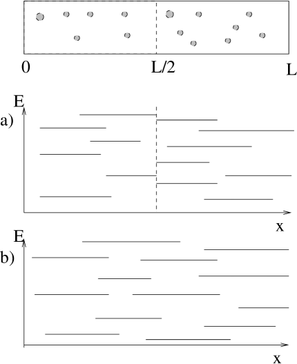
FIG. 2.: Schematic visualization of the energy level spectrum of localized states in a) a disordered quantum wire of length L, when divided into two parts, b) for the same wire when both parts are connected and the eigenstates are hybridized.

This relation can be proven directly. The ASD at zero frequency $\bar{C}(0)_{L}$ of the wire of length $L$, becomes, when the wire is divided into two parts, $\bar{C}(0)_{L/2}^{2}$. For $L\rightarrow\infty$, we find that the relative difference is:

$$f(L)=\frac{\bar{C}(0)_{L/2}^{2}}{\bar{C}(0)_{L}}-1=2p\exp(-LE_{G}/2),$$ (48)

exponentially decaying with the length $L$. Here $p$ is the degeneracy of the first excited state of $\bar{H}(\omega=0)$. $f(L)$ can be estimated, following an argument by Mott[37]: When the two halves of the wire get connected, see Fig. (2), the Eigenstates of the two separate halves become hybridized and the Eigenenergy of a state $\psi_{n}$ is changed by $\pm\Delta_{C}\exp(-2x_{n}/L_{C})$. $x_{n}$ is random, depending on the position of an eigenstate with closest energy in the other half of the wire. Thus, averaging over $x_{n}$ gives:

$$f(L)\sim+\exp(-4L/L_{C}).$$ (49)

Comparison with Eq. (48) yields indeed $1/L_{C}=8E_{G}$.

It is thus a remarkable fact that this length scale, defined as the crossover length of the spectral autocorrelation function, and related to the excitation gap of the compact nonlinear sigma model, has exactly the same symmetry dependence as the localization length, defined through the exponential decay of the spatial density correlation function, found in Ref. [3]. This is especially surprising, since the nonperturbative derivation of the disorder average of the quantity, $<\rho({\bf r},t)\rho({\bf r^{\prime}},t^{\prime})>-<\rho({\bf r})^{2}>$, necessitates the use of the supersymmetry method, resulting in a nonlinear sigma model of supermatrices, having in addition to a compact sector, the one considered here, a non compact sector, where the matrix is parametrized on a semi infinite interval. The full supersymmetry allows furthermore rotations between this compact and noncompact sector which are parametrized by Grassmann numbers $\xi$, having the property $\xi^{2}=0$. Apart from this increase of the manifold of the matrix fields $Q$ to the supersymmetric space, the structure of the theory is equivalent. Especially, the free energy of the supersymmetric nonlinear sigma model, has exactly the same form as Eq. (36), replacing $Q$ by supermatrices and the Trace over Q, by a supertrace $STr$, giving the opposite sign to the noncompact sector[2].

Studying localization in a wire with this supersymmetric nonlinear sigma model, the transfer matrix method yields an effective Hamiltonian of supermatrices $Q$, of the same form as Eq. (39), where the Laplacian is now defined on the respective supersymmetric manifold. In full analogy, the spectrum of $\bar{H}$ determines accordingly the properties of a disordered quantum wire, and has been derived in Ref. [36] for the pure ensembles. The partition function $Z=STr\exp(-L\bar{H})$ is a generating function of spectral correlation functions[38, 17]. In order to derive spatial correlation functions like the density correlation function, in addition, the Eigen functions of the respective diffusion equation on the supersymmetric manifold,

$$(-\partial_{x}+\bar{H}(Q))\psi(x;Q)=0,$$ (50)

have to be found[3]. In that way, a formula for the conductance of a finite disordered wire attached to two leads at a distance $L$, has been derived[36], see also Ref [2]. In the limit of a wire which is perfectly coupled to the leads, that formula for the average conductance simplifies to

$$<g>=\frac{1}{2\alpha}\int d\mu({l_{i}})E({l_{i}})\exp(-\frac{L}{16}E({l_{i}}).$$ (51)

Where $E({l_{i}})$ are the eigenvalues of the supersymmetric Hamitlonian $\bar{H}(\omega=0)$ and $d\mu({l_{i}})$ the corresponding integration measure, of the discrete and continous eigenvalues of the angular momentum operator on the compact and noncompact sector, respectively. They were found to be given for $B=0$ by[36]

$$E({l_{i}})=0,4/L_{CU}2(\epsilon^{2}+1),4/L_{CU}(l^{2}+\epsilon_{1}^{2}+\epsilon_{2}^{2}+1),$$ (52)

where $l=3,5,...$, and $\epsilon>0,\epsilon_{1}>0,\epsilon_{2}>0$.

For time reversal symmetry broken wires $X>1$ the eigenvalues were found to be,

$$E({l_{i}})=0,\frac{4}{\alpha L_{CU})}(l^{2}+\epsilon^{2}),$$ (53)

where $l=1,3,5,...$, and $\epsilon>0$.

If spin symmetry is broken, but time reversal symmetry conserved, in the presence of spin orbit scattering, the eigenvalues were found to be,

$$E({l_{i}})=0,\frac{4}{2L_{CU}}(2(l-1)^{2},\frac{4}{2L_{CU}}(l_{1}^{2}+l_{2}^{2}+\epsilon^{2}-1),$$ (54)

where $l=3,5,...$, $l_{i}=1,3,5,..,i=1,2$ and $\epsilon>0$.

In that case it can be seen that for a distance between the leads much exceeding the localizaion length, $L\gg L_{CU}$, the conductance decays exponentiallly, and that this is entirely determined by the compact gap $\tilde{E}_{\rm G}$, between the lowest angular momentum eigenstates of the compact sector. The integration over the continous eigenvalues of the noncompact sector, leads only to a prefactor, decaying as a power of the length, $\sim 1/L^{3/2}$. Indeed, the gap between the ground state value $E=0$ and the first excited state is seen from Eqs. (52,53,54), to be $\tilde{E}_{G}=8/L_{CU}$ for $B=0$, $\tilde{E}_{G}=4/L_{CU}$ for $X>1$, $\tilde{E}_{G}=2/L_{CU}$ for magnetic impurity scattering, $\alpha=2$, and $\tilde{E}_{G}=2/L_{CU}$ for moderate spin- orbit scattering, coinciding with the symmetry dependence of the compact gap derived above. However, that coincidence might appear as mere chance, since in fact, the Laplacian of the supersymmetric matrix $Q$ can not be written as a sum of the one of the respective compact nonlinear sigma model, Eqs. ( 40,43,45 ), because the metric tensor $\hat{g}$ on the supersymmetric space contains mixed factors of compact and noncompact parameters. Therefore, the discrete eigenvalues of $-\Delta_{Q}$, are not the Eigenvalues of the square of the angular momentum on a compact sphere[36]. Only, in the limit of infinite noncompact parameters does one recover the respective Laplacian on the compact symmetric space, Eqs. ( 40,43,45 ).

Thus, having shown that the ASD yields the correct symmetry dependence of the localization length, we can now use this approach to get an analytical solution for the crossover behaviour of the localization length and the local level spacing as a magnetic field is turned on, and there is no spin- orbit scattering. While a self consistent approach [39], a semiclassical analysis[40] and numerical studies[41, 42] showed a continous increase of the localization length, an analytical result [43] indicated that both limiting localization lengths $L_{c}(\beta=1)$ and $L_{c}(\beta=2)$ are present in the crossover regime and that there is no single parameter scaling. This is explained by arguing that the far tails of the wavefunctions do cover a large enough area to have fully broken time reversal symmetry, decaying with the length scale $L_{c}(\beta=2)$ even if the magnetic field is too weak to affect the properties of the bulk of the wavefunction, which does decay at smaller length scales with the shorter localization length $L_{c}(\beta=1)$, corresponding to the time reversal symmetric case. The quantity studied there is the imprurity averaged correlation function of local wavefunction amplitudes and its momenta at a fixed energy $\epsilon$: $Y(\epsilon)=<\sum_{\alpha}\mid\psi_{\alpha}(0)\mid^{2}\mid\psi_{\alpha}(r)\mid^{2}\delta(\epsilon-\epsilon_{\alpha})>$. It is averaged over a distribution of eigenfunctions in different impurity representations. Thus, each eigenfunction could decay exponentially with a single localization length, but having a distribution which has two maxima, at $L_{c}(\beta=1)$ and $L_{c}(\beta=2)$, whose weight is a function of the magnetic field in the crossover regime. While the distribution function of $\ln(\mid\psi_{\alpha}(0)\mid^{2}\mid\psi_{\alpha}(r)\mid^{2})$ is known to be Gaussian in both limiting cases of conserved, and fully broken time reversal symmetry, centered around the value $r/L_{C}(\beta)$, $\beta=1,2$, respectively, it is not yet known in this crossover regime, however[16]. The average value of moments, $\mid\psi_{\alpha}(0)\mid^{k}\mid\psi_{\alpha}(r)\mid^{k}$, is decaying more slowly than its typical value, and does not depend on the order of the moment,$k$. This was taken as a proof that moments are determined by states with anomalously large localization lengths of the order of the system size[16]. Therefore, the result of Ref. [43] can be a property of such rare states with anomalously large localization length, and it remains to see, if the full distribution function scales with two lengths $L_{c}(\beta)$, $\beta=1,2$, or a single one, changing continously with the magnetic field, $L_{c}(B)$.

While we cannot resolve this question by calculating a spectral autocorrelation function like the ASD, this is another motivation to see if the energy level statistics is governed by a single parameter as the magnetic field is varied.

The effective Hamiltonian for moderate magnetic fields is found, without spin dependent scattering, $\alpha=1$, using $Tr[Q,\tau_{3}]^{2}=16(1-\lambda_{C}^{2})$ to be given by:

$$\bar{H}=\frac{1}{L_{CU}}(-4\Delta^{R}_{Q}+X^{2}(1-\lambda_{C}^{2})),$$ (55)

where the Laplacian is Eq.(40) and $X=L_{CU}/(2L_{B})$.

In the limit $X\rightarrow 0$ the ground state and first excited state approach $1,\lambda_{C}\lambda_{D}$, respectively. In the limit $X\gg 1$, $\lambda_{C}^{2}$ becomes fixed to 1. Thus, the Ansatz $\psi_{0}(\lambda_{C})\sim\exp(A_{0}X^{2}(1-\lambda_{C}^{2}))$, and $\psi_{1}(\lambda_{C},\lambda_{D})\sim\lambda_{C}\lambda_{D}\exp(A_{1}X^{2}(1-\lambda_{C}^{2}))$, where $A_{0}<0,A_{1}<0$ are negative constants, solves $\bar{H}\psi=\bar{E}\psi$ to first order in $z=X^{2}(1-\lambda_{C}^{2})$. One finds that the two lowest magnetic field dependent eigenvalues are $E_{0}=4/L_{CU}(-5+\sqrt{25+X^{2}})$, and $E_{1}=4/L_{CU}(-3+\sqrt{49+X^{2}})$, and the Eigenfunctions are given as above with $A_{0}=-L_{CU}E_{0}/(16X^{2})$, and $A_{1}=(1-L_{CU}E_{1}/16)/X^{2}$, yielding the right limits for $X\rightarrow 0$ and $X\gg 1$, respectively. Thus, there is a magnetic field dependent gap $E_{G}=E_{1}-E_{0}$ of magnitude:

$$E_{G}(X)=4(2+\sqrt{49+X^{2}}-\sqrt{25+X^{2}})/L_{CU}.$$ (56)

This solution is valid in both the limits $X\ll 1$ and $X\gg 1$, interpolating the region $X\approx 1$.

With the magnetic diffusion length $L_{B}=(D\tau_{B})^{1/2}$, and the magnetic phase shifting rate, as given by Eq. (20), we obtain:

$$X=L_{CU}/(2L_{B})=L_{CU}\frac{q}{\hbar}\sqrt{<y\bullet y>}B,$$ (57)

which is $\sqrt{<y\bullet y>}/W$ times the number of flux quanta penetrating a localization area $L_{CU}W$.

From Eq. (56) follows that the magnetic change of the localization length is $\delta L_{C}(B)\sim B^{2}$ for small and $\sim 1/B$ at large magnetic fields, which agrees with the result of the selfconsistent method as obtained by Bouchaud[39].

VI Resistance of disordered Quantum Wires

In the limit of zero temperature, $T=0$, the resistivity of a disordered quantum wire, having only localized states at the Fermi energy, is infinite. For finite temperature, $T>0$, in the strong localization regime $k_{\rm B}T<\Delta_{\rm C}$, the mechanism of conduction is hopping of electrons between localized states. Then, the resistivity increases exponentially with temperature. According to the resistor network model[44, 45], each pair of localized states $i$ and $j$ is linked by a resistance $R_{ij}$:

$$R_{ij}=\exp(\frac{2r_{ij}}{L_{c}}+\frac{\epsilon_{ij}}{k_{B}T})$$ (58)

where $r_{ij}=|r_{i}-r_{j}|$ and $\epsilon_{ij}=(|\epsilon_{i}-\mu|+|\epsilon_{j}-\mu|+|\epsilon_{i}-\epsilon_{j}|)/2k_{B}T$ ($r_{i}$ and $\epsilon_{i}$ are the position and energy of the state $i$, $\mu$ being the Fermi energy). Because of the exponential dependence of $R$ on $r_{ij}$ and $\epsilon_{ij}$, percolation theory methods can be applied [46, 47, 48]. In 2-D and 3-D systems, the dependence of $R$ on temperature $T$ shows a crossover from an activated behaviour to the variable range hopping (VRH) regime. In this regime the temperature is so low that the typical resistances between neighbouring states are large because of the second term in Eq. (58). Therefore electrons tunnel to distant states whose energies are close to the Fermi level. If we neglect electron-electron interactions the resistivity is described by Mott’s law [49, 46]:

$$R(T)=R_{0}\exp[(\gamma T_{0}/T)^{1/(d+1)}]$$ (59)

where $d$ is the dimensionality of the system, $\gamma$ a numerical coefficient which depends on $d$, $T_{0}=1/\nu L_{c}^{d}$ and $\nu_{d}$ is the dimens dependent density of states. However, in the quasi-1-D case and for sufficiently long wires the variable range hopping result, Eq. (59), cannot used due to the presence of exponentially rare segments inside which all the localized states have energies far from the Fermi level [50, 51, 52]. These large resistance segments (LRS) do not strongly affect the resistivity of 2-D and 3-D systems because they can be circumvented by the current lines. In 1-D this is not possible and the total resistance of a wire is given by the sum of the resistances of all the LRS’s. This sum yields an activated type dependence of $R$ on $T$[51] for infinite wires:

$$R=R_{0}\frac{L}{L_{c}}(\frac{T_{0}}{T})^{\frac{1}{2}}\exp(T_{0}/2T),$$ (60)

where $k_{\rm B}T_{0}=1/\nu L_{c}=\Delta_{\rm c}$ coincides with the local level spacing, and $L$ is the length of the wire. Eq. (60) is valid provided that the number of optimal LRS’s (i.e. those LRS’s which give the largest contribution to $R$ [51]) within the length of the sample) is large. Bur for a finite wire length this condition fails to be fulfilled at very low temperature $T$, and the resistance of the chain is determined by smaller LRS’s; in this regime Eq. (60) is replaced by [50, 51]:

$$R\approx R_{0}\exp[\sqrt{2\frac{T_{0}}{T}\log(\frac{L}{L_{c}}(\frac{T}{T_{0}})^{\frac{1}{2}}\log^{\frac{1}{2}}(\frac{L}{L_{c}}))}],$$ (61)

which is valid below a temperature

$$T_{1}=\frac{T_{0}}{2\ln(L/L_{c})},$$ (62)

approaching Mott’s law, Eq. (59) at lower temperatures $T<T_{1}$.

So far, electron-electron interactions have not been taken into account. This approximation is valid if the Coulomb interaction is screened over distances of the order of the hopping length, as by a metal gate electrode deposited on top of the wires at a distance smaller than the typical hopping lengths. When this is not the case, long range electron-electron interactions affect both the density of states and the resistance of the samples [53, 54].

VII Comparison with experimental results

The magnetic field dependent activation energy was measured recently in transport experiments of Si $\delta$- doped Ga As quantum wires[4]. As an example, we discuss here the sample 5 of Ref. [4], with a width $W=.2\mu m$, a localization length $L_{CO}=.61\mu m$ a length $L=40\mu m$, and $N=30$ channels.

The activation energy coincides with the local level spacing $k_{\rm B}T_{0}=\Delta_{c}=1/(\nu WL_{c})$ and is estimated for sample 5 to be $T_{0}=.34K$.

Thus, according to the theory outlined in the previous section, there is an activated reistance in an order of magnitude temperature range $T_{1}=.04K<T<T_{0}=.34K$, allowing in good approximation the direct measurement of the magnetic field dependent activation energy $\Delta_{c}(B)$, and thus the magnetic field dependence of the localization length $L_{C}(B)$.

The ratio of the cyclotron frequency and the elastic scattering rate, $\omega_{C}\tau=l/(k_{\rm F}l_{B}^{2})\ll 1$, is small in the whole range of magnetic fields considered there, so that the classical conductance would be magnetic field independent, $\sigma=ne^{2}\tau/m(1+\omega_{C}^{2}\tau^{2})^{-1}\approx ne^{2}\tau/m$.

The mean free path $l\sim.02\mu$ is small compared to the width of the sample $W=.2\mu m$. The magnetic length is $l_{B}=.026\mu m(B/T)^{-1/2}$. Thus, while $\omega_{C}\tau\ll 1$, the magnetic length becomes smaller than the width of the sample at magnetic fields $B>.0165T$.

The experimental magnetic field dependence of the ratio of activation energies is shown in Fig. (3) together with the theoretical curve for the ratio of local energy level spacings $\Delta_{C}(B)/\Delta_{C}(0)=E_{G}(B)/E_{G}(0)$, as derived above, Eq. ( 36 ), using for the magnetic phase shifting rate the results for a 2-dimensional wire with specular boundary conditions, Eq. (14), and, for comparison, the one derived for a parabolic wire, Eq. (32).

There is a quantitative discrepancy between the best fit $X=.036B/G$, and $X=2\pi\phi/\phi_{0}$, $\phi=\mu_{0}HL_{CU}(\overline{y^{2}})^{(1/2)}$, when using the analytical formula Eq. ( 14). With the experimental parameters $\alpha=1,L_{CO}=.61\mu m$, width $W=.2\mu m$ of sample 5 in Ref. [4] and $\overline{y^{2}}=W^{2}/12$ for a 2- dimensional wire, it yields rather $X=.010B/G$. We note that smooth confinement can give $\overline{y^{2}}>W^{2}/12$. A similar discrepancy was observed between $W$ as obtained from the sample resistance and estimated from the analysis of the weak localization magnetoresistance, which also depends on $\overline{y^{2}}$[55].

We note that the agreement, when using the experimental parameters, for the parabolic wire, is better. The cyclotron length $l_{\rm cyc}=k_{\rm F}l_{\rm B}^{2}=.32/(B/T)\mu m$, is found to be larger than the mean free path $l$ for $B<15T$ and larger than the wire width for $B<1.5T$. We find for the parabolic wire: $X=.024(.99+1.33~{}10^{-8}(B/G)^{2})^{1/2}B/G$. The enhancement of the magnetic phase shifting rate in a parabolic wire, Eq. (32), is thus too weak to be seen at the magnetic fields used in the experiment, $B<.2T$, as shown in Fig. (3), and seems thus not to be the origin of the increase in the decay of the activation gap, at about $.1T$ .

An extension of the derivation given in section IV to include a dependence of the eigenfunctions on the magnetic field also for a 2-dimensional wire with specular boundary conditions has to be done, in order to make the comparison with the experiment more quantitative, and conclude from the magnetolocalization on the form of the confinement potential in these Si- $\delta$- doped Ga As quantum wires. But, our results may indicate that the harmonic confinement model of the parabolic wire is a better description of the wires in sample 5.

FIG. 3.: The activation gap ratio $T_{0}(H)/T_{0}(0)$ as a function of the magnetic field $B$ in $G$ of sample 5 measured at temperature $T=.3K$ as reported in Ref. 1, together with the theoretical curves for a parabolic wire, using the parameters of sample 5. and a 2D wire with specular boundary conditions for a best fit value $X=.036B/G$, and the value obtained from the experimental parameters, $X=.010B/G$.

VIII Summary and open problems

A formula for the magnetic phase shifting rate has been derived, which allows its calulcation for arbitrary wire geometries and ratios of the elastic mean free path, the wire width, and the magnetic length.

For a quantum wire with specular boundary conditions and harmonic confinement this formula has been evaluated explicitly, and compared with previous analytical and numerical results for the magnetic phase shifting rate.

The localization length is derived as the crossover length scale from correlated to uncorrelated energy level statistics, as studied with the autocorrelation function of spectral determinants. It is shown that its symmetry dependence coincides exactly with the localization length as defined by the exponential decay of the averaged two-terminal conductance and derived with the supersymmetry method.

Therefore, the ASD can be used to get analytical information on the magnetic field dependence of the localization length, which is shown to be governed by the magnetic phase shifting rate, and thus strongly dependent on the geometry of the wire and the ratios of the elastic mean free path, the wire width, and the magnetic length.

A comparison with the magnetic field dependence of the activation gap, as observed in low temperature resistance measurements in Si $\delta$- doped Ga As wires, indicates, that the electrons move in a potential which is closer to a harmonic than a hard wall confinement.

Enhancement of the sensitivity of the localization to a magnetic field is found analytically, when the cyclotron length is comparable with its width. The physical reason for this enhancement is found to be the magnetic field dependent shift of the guiding centers of the electronic eigenstates in the quantum wire, even at moderate magnetic fields, when the classical conductivity is still independent of the magnetic field.

It remains to extend the derivation to include random surface scattering [41] and the effect of correlated, smooth disorder[57], in order to allow for a more quantitative comparison with the experiment. Both effects necessitate a new derivation of the nonlinear sigma model, which allows for a directional dependence of the matrix field $Q$. This has been recently introduced for a system with broken time reversal symmetry in the study of localization in correlated disorder [34], and the spectral statistics of quantum billards with surface scattering[35]. In both cases one is lead to a nonlinear sigma model, where variations of the matrix $Q$ on ballistic length scales are taken into account[58, 59, 60]. The application of this approach to the magnetolocalization in disordered quantum wires will be presented in a future publication.

Appendix A

Here, the derivation for spinless case, $\alpha=1$, is given in detail. We use for compactness the vectors of anticommuting variables,

$$\psi({\bf x})=\left(\begin{array}[]{c}\xi({\bf x})\\ \xi^{*}({\bf x})\\ \eta({\bf x})\\ \eta^{*}({\bf x})\end{array}\right),\bar{\psi}({\bf x})=(\xi^{*}({\bf x}),-\xi({\bf x}),\eta^{*}({\bf x}),-\eta({\bf x})).$$ (63)

Note that $\bar{\psi}=(C\psi)^{T}$, where the matrix $C$ interchanges the Grassmann fields with their conjugate one, and has thus the form $C=\left(\begin{array}[]{cccc}0&-1&0&0\\ 1&0&0&0\\ 0&0&0&-1\\ 0&0&1&0\end{array}\right)$.

Thus, the ASD is written as

$$\bar{C}(\omega) = \int\prod_{\bf x}d\psi({\bf x})$$ (65)

$$\exp(-\frac{1}{2}\int d{\bf x}\bar{\psi}({\bf x})(E+\frac{1}{2}\omega\Lambda-\hat{H_{0}}-V({\bf x}))\psi({\bf x})),$$

Here, the diagonal Pauli matrix $\Lambda=\left(\begin{array}[]{cc}1&0\\ 0&-1\end{array}\right)$ has been introduced for compactness, its diagonal elements projecting on the respective spectral determinant of the ASD. The kinetic Hamiltonian becomes a matrix

$$\hat{H_{0}}=(\hat{p}-q\tau_{3}{\bf A})^{2}/2/m,$$ (66)

where the diagonal Pauli matrix $\tau_{3}$ had to be introduced since each vector has elements of the Grassmann field and the time reversed one, and the diamagnetic term ${\bf pA}/m$ in the Hamiltonian changes sign, as ${\bf p}\rightarrow-{\bf p}$, breaking the time reversal invariance.

To summarize the notation, here, and in the following, $\Lambda_{i}$ are the Pauli matrices in the subbasis of the left and the right spectral determinant, $\tau_{i}$ the ones in the subbasis spanned by time reversal and $\sigma_{i}$ the ones in the subspace spanned by the spinor, for $i=1,2,3$.

Note that a global transformation of the Grassmann vectors $\psi\Rightarrow\tilde{\psi}=A\psi$ does leave the functional integral for $\omega=0$ invariant, as long as $A^{+}A=1$, and $A^{+T}C=CA$, restricting the matrices $A$ to be symplectic ones, being elements of $Sp(2)$, commuting with the antisymmetric matrix $C$. A finite frequency breaks this symmetry group, and only symplectic transformations of each field of a single spectral determinant separately, $Sp(1)\times Sp(1)$, do leave the functional integral invariant.

Now, the averaging over the disorder potential can be done, integrating Eq. (65) over the Gaussian distribution function of the random potential V.

Thus, the averaged ASD is found to be given by a functional integral over interacting Grassman fields $\psi$,

$$\bar{C}(\omega) = \int\prod_{\bf x}d\psi({\bf x})$$ (69)

$$\exp(-\frac{1}{2}\int d{\bf x}\bar{\psi}({\bf x})(E+\frac{1}{2}\omega\Lambda-\hat{p}^{2}/2/m)\psi({\bf x}))$$

$$\exp(-\frac{1}{16\pi}\frac{\hbar\Delta}{\tau}SL\int d{\bf x}Tr(\psi({\bf x})\times\bar{\psi}({\bf x}))^{2}).$$

Now, the resulting $\psi^{4}$-interaction term can be decoupled by introducing another Gaussian integral over an auxilliary field. Clearly, the field should not be a scalar, otherwise we would simply reintroduce the Gaussian integral over the random potential $V$. Rather, in order to go a step forward, the auxilliary field should capture the full symmetry of the autocorrelation function. Therefore, the Gaussian integral is chosen to be over a 4 by 4 matrix $Q_{4\times 4}$, which is itself an element of the respective symmetric space, as the matrix $A$ which leaves the functional integral invariant. Thus, allowing for a spatial dependence of $Q$, one can decouple the interaction term:

$$\exp(-\frac{1}{16\pi}\frac{\hbar\Delta}{\tau}SL\int d{\bf x}(\psi({\bf x})\times\bar{\psi}({\bf x}))^{2})$$ (70)

$$= \int\prod_{x}dQ_{4\times 4}({\bf x})\exp(-\pi\frac{\tau}{\hbar\Delta}\int\frac{d{\bf x}}{SL}TrQ_{4\times 4}({\bf x})^{2}$$ (71)

$$+ i\frac{1}{2}\int d{\bf x}TrQ_{4\times 4}({\bf x})\psi({\bf x})\times\bar{\psi}({\bf x})).$$ (72)

Anticipating, however, that the functional integral over the matrices $Q$ cannot be performed exactly, but rather only an integral over slowly varying modes around a saddle point solution, it is necessary to separate fast and slowly varying modes already before the decoupling of the interaction term Eq. (70)[22]. It turns out that there are two equivalent slowly varying interaction terms, corresponding to diffusion, and one arrives finally after a Gaussian decoupling to a, by a factor $1/2$, shallower nonlinear coupling $TrQ^{2}$[2].

Next, one can perform the Gaussian integral over the Grassmann vectors $\psi({\bf x})$ and one obtains for the ASD, rescaling $Q_{4\times 4}\rightarrow 2\tau/\hbar Q_{4\times 4}$, the representation:

$$\bar{C}(\omega)=\int\prod dQ_{4\times 4}({\bf x})\exp(-F[Q]),$$ (73)

with

$$F[Q]= \frac{\pi}{8}\frac{\hbar}{\Delta\tau}\int\frac{d{\bf x}}{SL}TrQ_{4\times 4}({\bf x})^{2})$$ (75)

$$+\frac{1}{2}\int d{\bf x}<{\bf x}\mid Tr\ln(G(\hat{x},\hat{p})\mid{\bf x}>,$$

where

$$G(\hat{x},\hat{p})=1/(\frac{1}{2}\omega\Lambda-\frac{(\hat{p}-q\tau_{3}A)^{2}}{2m}+i\frac{\hbar}{2\tau}Q_{4\times 4}(\hat{x})).$$ (76)

is the propagator matrix. We used the operator notation $\hat{x}$, in order to stress that the terms in the inverse propagator, do not commute with each other.

Appendix B

For a clean wire with hard wall boundaries, the transversal Eigen modes are for $-W/2<y<W/2$, $<k_{y}\mid y>=\cos k_{y}y$ for $k_{y}=\pi s/W$, $s$ being an odd integer, and $<k_{y}\mid y>=\sin k_{y}y$ for $k_{y}=\pi s/W$, s being an even integer, one obtains:

$$\mid<k_{y}\mid y\mid k_{y}^{\prime}>\mid^{2}=\frac{1}{W^{2}}(\frac{1}{(k_{y}-k_{y}^{\prime})^{2}}-\frac{1}{(k_{y}+k_{y}^{\prime})^{2}})^{2},$$ (77)

when $k_{y}=\pi s/W$, and $k_{y}^{\prime}=\pi s^{\prime}/W$, s being even, and s’ odd, or vice versa. Then, the sum over $k_{y}^{\prime}$ in Eq. ( 21 ) can be performed by use of the Matsubara trick, for $s$ even, and odd integers, separately. The remaining sum over $k_{x},k_{y}$ can be transformed as $1/(WL)\sum_{k_{x},k_{y}}=\int d\epsilon\nu(\epsilon)\int\frac{d\hat{e}_{k}}{\Omega_{k}}$, noting that the unit vector $\hat{e}_{k}$ can point only in discrete directions. Thus, while in 2 dimensions $\int\frac{d\hat{e}_{k}}{\Omega_{k}}=\int_{0}^{2\pi}\frac{d\theta}{2\pi}=4/(2\pi)\int_{0}^{1}dy1/(1-y^{2})^{(}1/2)$, for finite number of transverse channels $N=k_{F}W/\pi$ there is a sum, $\int\frac{d\hat{e}_{k}}{\Omega_{k}}=2/(\pi N)\sum_{s>0}1/(1-s^{2}/N^{2})^{(}1/2)$. Thus, $k_{y}=\pi s/W=k_{F}s/N$ and $k_{x}=k_{F}(1-s^{2}/N^{2})^{(}1/2)$. Performing finally for $E\gg\hbar/\tau$ the integral over $\epsilon$, one arrives with some patience at Eq. (22), where $K_{0}=2/(\pi N)\sum_{s=0}^{N}\sqrt{1-\frac{s^{2}}{N^{2}}}$, $K=2/(\pi N)\sum_{s=1}^{N}\sqrt{1-\frac{s^{2}}{N^{2}}}$, $K_{1}=2/(\pi N)\sum_{s=1}^{N}\sqrt{1-\frac{s^{2}}{N^{2}}}/s^{2}$, $K_{2}=2/(\pi N)\sum_{s=1}^{N}\sqrt{1-\frac{s^{2}}{N^{2}}}s^{2}/N^{2}$.

Appendix C

In order to derive the Laplacian in the respective representation of the matrix field $Q$, its general definition in an arbitrary parametrization,

$$\Delta_{Q}=\frac{1}{\sqrt{\bar{g}}}\sum_{i,k}\partial_{k}g^{ik}\sqrt{\bar{g}}\partial_{i},$$ (78)

where the matrix $g$ is the metric tensor, being defined by the quadratic form $ds^{2}=1/4TrdQ^{2}$ of the representation

$$ds^{2}=d{\bf x}^{T}gd{\bf x},$$ (79)

where ${\bf x}$ is the vector of parameters of the representation.

For $B\neq 0$, $Q$ is element of $U(2)/(U(1)\times U(1))$, by enforcing the conditions $Q^{2}=1$, $Q^{T}C=CQ$, and $Q^{+}=Q$, $[Q,\tau_{3}]=0$.

It can be paramterized as $Q=\left(\begin{array}[]{cc}\cos\theta&e^{i\chi}\sin\theta\\ e^{-i\chi}\sin\theta&-\cos\theta\end{array}\right)$

where $\theta\in[0,\pi]$ and $\chi\in[0,2\pi]$.

Thus,

$$ds^{2}=d\theta^{2}+\sin^{2}\theta d\chi^{2}.$$ (80)

and $g=\left(\begin{array}[]{cc}1&0\\ 0&\sin^{2}\theta\end{array}\right)$. Thus, with Eq. (78) follows:

$$\Delta_{Q}=\partial_{\lambda_{D}}(1-\lambda_{D}^{2})\partial_{\lambda_{D}}+\frac{1}{1-\lambda_{D}^{2}}d\chi^{2},$$ (81)

where $\lambda_{D}=\cos(\theta)$.

Note that the autocorrelation function depends on the energy difference $\omega$ through the coupling $Tr\Lambda Q=2*2\lambda_{D}$, so that only that part of the Laplacian which does not commute with $Tr\Lambda Q$,

$$\Delta^{R}_{Q}=\partial_{\lambda_{D}}(1-\lambda_{D}^{2})\partial_{\lambda_{D}}.$$ (82)

enters in the frequency dependence of the autocorrelation function of spectral determinants, Eq. ( 38 ). Since $U(2)/(U(1)\times U(1))=S_{2}$, the two sphere, this is equivalent to the treatment of spherically symmetric potentials, and the Laplacian can be identified with the square of the angular momentum, $-\Delta_{Q}={\bf L}^{2}$, and $L_{z}=i\partial_{\chi}/(1-\lambda_{D}^{2})$ does commute with the Hamiltonian,

$$\bar{H}=-1/(2m)L^{2}+i\alpha\frac{\pi}{4}\frac{\omega}{\Delta}z,$$ (83)

since $z=\cos\theta_{D}$ does commute with $L_{z}$. Therefore, $\omega\neq 0$ does not break the azimuthal symmetry of rotations around the z-axis, $n_{z}$.

For $B=0$, $Q$ is element of the symplectic symmetric space, $Sp(2)/(Sp(1)\times Sp(1))$, by enforcing the conditions $Q^{2}=1$, $Q^{T}C=CQ$, and $Q^{+}=Q$.

One obtains:

$$Q=\left(\begin{array}[]{cc}c\openone&A\\ A^{+}&-c\openone\end{array}\right).$$ (84)

with $A=\left(\begin{array}[]{cc}a&b\\ b^{*}&-a^{*}\end{array}\right)$ where $\mid a\mid^{2}+\mid b\mid^{2}+c^{2}=1$.

A matrix Q with the above symmetries can be represented as,

$$Q=U^{-1}Q_{c}^{0}U,$$ (85)

with

$$U=V_{C}U_{D},$$ (86)

where

$$U_{D}=V_{D}^{-1}T_{D}^{0}V_{D},$$ (87)

where

$$Q_{c}^{0}=\left(\begin{array}[]{cc}\cos\theta_{C}&i\sin\theta_{C}\tau_{2}\\ i\sin\theta_{C}\tau_{2}&-\cos\theta_{C}\end{array}\right),$$ (88)

and

$$T_{D}^{0}=\left(\begin{array}[]{cc}\cos\theta_{D}/2&i\sin\theta_{D}/2\\ i\sin\theta_{D}/2&\cos\theta_{D}/2\end{array}\right).$$ (89)

and

$$V_{C,D}=\left(\begin{array}[]{cc}\exp(i\phi_{C,D}\tau_{3})&0\\ 0&\openone\end{array}\right).$$ (90)

and $\tau_{i},i=1,2,3$ are the Pauli matrices. Such a representation was first given by Altland, Iida and Efetov[61] to study the crossover between the spectral statistics of Gaussian distributed random matrices as the time reversal symmetry is broken, within the supersymmetric nonlinear sigma model. Here, in order to study the ASD, we need to consider only the compact block of the representation given there.

We find that $ds^{2}=TrdQ^{2}/4=d\theta_{C}^{2}+\cos^{2}\theta_{C}d\theta_{D}^{2}+\sin^{2}\theta_{C}\phi_{C}^{2}+\cos^{2}\theta_{C}\sin^{2}\theta_{D}d\phi_{D}^{2}$ and thereby with Eq. (78 ), the part of the Laplace operator which does not commute with $Tr\lambda Q=4\lambda_{C}\lambda_{D}$ is given by Eq. ( 40),

$$\Delta^{R}_{Q} = \partial_{\lambda_{C}}(1-\lambda_{C}^{2})\partial_{\lambda_{C}}+2\frac{1-\lambda_{C}^{2}}{\lambda_{C}}\partial_{\lambda_{C}}$$ (91)

$$+ \frac{1}{\lambda_{C}^{2}}\partial_{\lambda_{D}}(1-\lambda_{D}^{2})\partial_{\lambda_{D}},$$ (92)

where $\lambda_{i}=\cos\theta_{i},i=C,D$.

For moderately strong spin- orbit scattering $1/\tau_{SO}>\Delta_{C}$, in the functional integral representation of the spectral determinants by Grassman vectors the spin degree of freedom is introduced, $\alpha=2$ and the matrix $C$ is, due to the time reversal of the spinor, substituted by $i\sigma_{2}\tau_{1}$[22]. The spin-orbit scattering reduces the Q matrix to unity in spin space. Thus, the matrix C has effectively the form $\tau_{1}$. The condition $Q^{T}C=CQ$ leads therefore to a new symmetry class, when the spin symmetry is broken but the time reversal symmetry remains intact. Then, $Q$ are $4\times 4$- matrices on the orthogonal symmetric space $O(4)/(O(2)\times O(2))$ [28].

A matrix $Q$ with the above symmetries can be represented as,

$$Q=V^{-1}Q_{0}V,$$ (93)

with

$$Q_{c}^{0}=\left(\begin{array}[]{cc}\cos\hat{\theta}&\sin\hat{\theta}\par\\ \sin\hat{\theta}&-\cos\hat{\theta}\end{array}\right),$$ (94)

where

$$\hat{\theta}=\left(\begin{array}[]{cc}\theta_{1}&\theta_{2}\\ \theta_{2}&\theta_{1}\end{array}\right),$$ (95)

with $\theta_{i}\in[0,\pi],i=1,2$, and

$$V=\left(\begin{array}[]{cc}V_{1}&0\\ 0&V_{2}\end{array}\right),$$ (96)

where

$$V_{i}=\exp(i\chi_{i}\tau_{3}),$$ (97)

with $\chi_{i}\in[0,2\pi],i=1,2$.

Thus, we find $ds^{2}=TrQ^{2}/4=\sum_{i=1,2}d\theta_{i}^{2}+d{\bf\chi}^{T}\hat{g_{\chi}}{\bf\chi}$, where

$$\hat{g_{\chi}}=\left(\begin{array}[]{cc}\sin^{2}\theta_{1}+\sin^{2}\theta_{2}&-\sin^{2}\theta_{1}+\sin^{2}\theta_{2}\\ -\sin^{2}\theta_{1}+\sin^{2}\theta_{2}&\sin^{2}\theta_{1}+\sin^{2}\theta_{2}\end{array}\right),$$ (98)

Thus, the part of the Laplace operator which does not commute with $Tr\lambda Q=4\lambda_{1}\lambda_{2}$ is given by Eq. ( 45),

$$\Delta^{R}_{Q}=\sum_{l=1,2}\partial_{\lambda_{l}}(1-\lambda_{l}^{2})\partial_{\lambda_{l}},$$ (99)

where $\lambda_{i}=\cos\theta_{i},i=1,2$.

REFERENCES

- [1] P.A. Lee, T.V. Ramakrishnan, Rev. of Mod. Phys. 57, 287 (1985); B. Kramer and A. MacKinnon, Rep. Prog.Phys. 56, 1469 (1993); C. W. J. Beenakker, Rev. Mod. Phys. 69, 731 (1997).
- [2] K. B. Efetov, Supersymmetry in Disorder and Chaos Cambridge University Press, Cambridge (1997).
- [3] K. B. Efetov, A. I. Larkin, Zh. Eksp Teor. Fiz. 85, 764(1983) ( Sov. Phys. JETP 58, 444 ).
- [4] M. E. Gershenson et al., Phys. Rev. Lett. 79, 725(1997); Phys. Rev. B 58, 8009 (1998).
- [5] B. L. Altshuler, A. G. Aronov, Pis’ma Zh. Eksp. Teor. Fiz. 33, 515 (1981)[JETP Lett. 33,499 (1981)].
- [6] V. K. Dugaev, D.E. Khmel’nitskii, Sov. Phys. JETP 59, 1038 (1984).
- [7] B. L. Altshuler, A.G. Aronov in Electron-electron interactions in disordered systems, North Holland (1985).
- [8] C. W. J. Beenakker, H. van Houten, Phys. Rev. B 37, 6544 (1988).
- [9] F. Haake, M. Kus, H.- J. Sommers, H. Schomerus, and K. Zychowski, J. Phys. A 29, 3641(1996).
- [10] S. Kettemann, D. Klakow, U. Smilamsky, J. Phys. A,3643(1997).
- [11] F. J. Dyson, J. Math. Phys. 3, 1199 (1962).
- [12] K. B. Efetov, Zh. Eksp. Teor. Fiz. 83, 833 (1982)[Sov. Phys. JETP 56,467 (1982)]; J. Phys. C 15, L 909 (1982).
- [13] L. P. Gor’kov, O. N. Dorokhov, and F. V. Prigara, Zh. Eksp. Teor. Fiz. 84, 1440 (1983)[Sov. Phys. JETP 57, 838 (1983)]. B. L. Alt’shuler, B. I. Shklobskii, Zh. Eksp. Teor. Fiz. 91, 127 (1986)[Sov. Phys. JETP 64,127 (1986)].
- [14] B. L. Altshuler, I. Kh. Zharekeshev, S. A. Kotochigova, and B. I. Shklovskii, Zh. Eksp. Teor. Fiz. 94, 343 (1988)[Sov. Phys. JETP 67, 625 (1988)]; S. N. Evangelou, and E. N. Economou, Phys. Rev. Lett. 68, 361 (1992); E. Hofstetter, and M. Schreiber, Phys. Rev. Lett. 73, 3137 (1994); I. Kh. Zharekeshev, and B. Kramer, Phys. Rev. Lett. 79, 717(1997).
- [15] A. Altland, D. Fuchs, Phys. Rev. Lett. 74, 4269(1995).
- [16] A. D. Mirlin, Phys. Rep. 326, 259 (2000), Procy. of Intern. School of Physics ” Enrico Fermi”, Course CXLIII, IOS Press, Amsterdam ( 2000 ).
- [17] T. Guhr, A. M ller-Groeling, and H.A. Weidenm ller, Phys. Rep. 299, 189 (1998).
- [18] S. Kettemann, Phys. Rev. B 59 , 4799 (1999).
- [19] E. Abrahams, P. W. Anderson, D. C. Licciardello, V. Ramakrishnan, Phys. Rev. Lett 42 673(1979).
- [20] L. P. Gor’kov, A. I. Larkin, D. E. Khmel’nitskii, Pis’ma Zh. Eksp. Teor. Fiz. 30 , 248 (1979) ( JETP Lett. 30, 228 (1979)).
- [21] B. L. Altshuler, D. E. Khmelmitskii, A. I. Larkin, and P. A. Lee, Phys. Rev. B 22, 5142 (1980).
- [22] K. B. Efetov, A. I. Larkin, D. E. Khmel’nitskii, Zh. Eksp. Teor. Fiz. 79, 1120(1980) ( Sov. Phys. JETP 52, 568(1980) ).
- [23] S. Chakravarty, A. Schmid, Physics Reports 140, 193(1986).
- [24] B. L. Altshuler, A. G. Aronov, D.E. Khmelnitskii, J. Phys. C 15, 7367 (1982).
- [25] M. E. Gershenson, Ann. Phys. 8,559 (1999).
- [26] M. Buettiker, cond-mat/0105519 (2001).
- [27] S. Hikami, A. I. Larkin and Y. Nagaoka, Prog. Theor. Phys. 63, 707 (1980).
- [28] F. Wegner, Z. Physik B 36,l209(1979); Nucl. Phys. B 316, 663(1989); S. Hikami, Prog. Theor. Phys. 64, 1466 (1980).
- [29] S. Kettemann and A. Tsvelik, Phys. Rev. Lett. 82, 3689 (1999).
- [30] S. Kettemann, Phys. Rev. Rapid Commun. B 62 , R13282 (2000).
- [31] S. Helgason, Differential Geometry and Symmetric Spaces Academic Press, New York (1962).
- [32] M. R. Zirnbauer Jy. Math. Phys. 37,4986 (1996).
- [33] M. Titov, P. W. Brouwer, A. Furusaki, C. Mudry, cond-mat/0011146.
- [34] D. Taras- Semchuk, K. B. Efetov, Phys. Rev. Lett. 85, 1060 (2000); cond-mat/0010282 (2001).
- [35] Ya. M. Blanter, A. D. Mirlin, B. A. Muzykantskii, cond-mat/0011498 (2000).
- [36] M. R. Zirnbauer Phys. Rev. Lett. 69,1584 (1992), A. D. Mirlin, A. Mullergroeling, M. R. Zirnbauer, Ann. Phys. ( New York) 236, 325 (1994); P. W. Brouwer, K. Frahm, Phys. Rev. B 53 ,1490 (1996); B. Rejaei, Phys. Rev. B 53, R13235 (1996), B. Rejaei, Phys. Rev. B 53, R13235 (1996).
- [37] N. F. Mott, E. A. Davis, Electronic Processes in Non-crystalline Materials, Clarendon Press, Oxford (1971).
- [38] A. V. Andreev and B. D. Simons Phys. Rev. Lett. 75, 2304-2307 (1995).
- [39] J. P. Bouchaud, J. Phys. 1 (France) 1, 985 (1991).
- [40] I. V. Lerner, Y. Imry, Europhys. Lett. 29, 49(1995).
- [41] M. Leadbeater, V. I. Falko, C. J. Lambert,Phys. Rev. Lett. 81, 1274 (1998).
- [42] J.-L. Pichard, M. Sanquer, K. Slevin, and P. Debray, Phys. Rev. Lett. 65, 1812 (1990); H. Schomerus and C.W. Beenakker, Phys. Rev. Lett. 84, 3927 (2000); M. Weiss, T. Kottos, T. Geisel, Phys. Rev. B 63, R081306(2001).
- [43] A.V. Kolesnikov and K.B. Efetov, Phys. Rev. Lett. 83, 3689 (1999); A.V. Kolesnikov and K.B. Efetov, cond-mat/0005048 (to be published).
- [44] A. Miller and E. Abrahams, Phys. Rev. 120 , 745 (1960).
- [45] B. I. Shklovskii and A. L. Efros, Electronic Properties of Doped Semiconductors, Springer-Verlag, New York (1984).
- [46] V. Ambegaokar, B. I. Halperin and J. S. Langer, Phys. Rev. B4 , 2612 (1971).
- [47] M. Pollak, J. Non-Crystal. Solids 11 , 1 (1972).
- [48] B. I. Shklovskii and A. L. Efros, Zh. Eksp. Teor. Fiz. 60 , 867 (1971) [Sov. Phys. JETP 33 , 468 (1971)].
- [49] N. F. Mott, J. Non-Crystal. Solids 1 , 1 (1968).
- [50] P. A. Lee, Phys. Rev. Lett.53 , 2042 (1984); R. A. Serota, R. K. Kalia and P. A. Lee, Phys. Rev. B 33 , 8441 (1986).
- [51] M. E. Raikh and I. M. Ruzin, Zh. Eksp. Teor. Fiz. 95 , 1113 (1989) [Sov. Phys. JETP 68 , 642 (1989)].
- [52] J. Kurkijarvi, Phys. Rev. B8 , 922 (1973).
- [53] M. E. Raikh and A. L. Efros, Pis’ma Zh. Eksp. Teor. Fiz. 45 , 225 (1987) [JETP Lett. 45 , 280 (1987)].
- [54] A. I. Larkin and D. E. Khmel’nitskii, Zh. Eksp. Teor. Fiz. 83 , 140 (1982) [Sov. Phys. JETP 56 , 647 (1982)].
- [55] Yu. B. Khavin, M. E. Gershenson, A. L. Bogdanov, Phys. Rev. Lett. 81, 1066 (1998).
- [56] A. Altland, S. Iida, K. B. Efetov, J. Phys. A 26 (1993) 3545.
- [57] I. L. Aleiner, A. I. Larkin, Phys. Rev. B 54, 14423 (1996).
- [58] B. A. Muzykantskii, D. E. Khmelnitskii, JETP Letters 62,76 (1995)].
- [59] A. V. Andreev, O. Agam, B. D. Simons, and B. L. Altshuler, Phys. Rev. Lett. 76, 3947 (1996). Nucl. Phys. B 482, 536 (1996).
- [60] B. D. Simons, O. Agam, A. V. Andreev, J. Math. Phys. 38, 1982 (1997).
- [61] A. Altland, S. Iida, K. B. Efetov, J. Phys. A 26 (1993) 3545.