Theory of ARPES intensities from the CuO₂ plane

Abstract

We present a theory for the photon energy and polarization dependence of ARPES intensities from the CuO₂ plane in the framework of strong correlation models. We show that for electric field vector in the CuO₂ plane the ‘radiation characteristics’ of the $O$ $2p_{\sigma}$ and $Cu$ $3d_{x^{2}-y^{2}}$ orbitals are strongly peaked along the CuO₂ plane, i.e. most photoelectrons are emitted at grazing angles. This suggests that surface states play an important role in the observed ARPES spectra, consistent with recent data from Sr₂CuCl₂O₂. We show that a combination of surface state dispersion and Fano resonance between surface state and the continuum of LEED-states may produce a precipitous drop in the observed photoelectron current as a function of in-plane momentum, which may well mimic a Fermi-surface crossing. This effect may explain the simultaneous ‘observation’ of a hole-like and an electron-like Fermi surfaces in Bi2212 at different photon energies. We show that by suitable choice of photon polarization one can on one hand ‘focus’ the radiation characteristics of the in-plane orbitals towards the detector and on the other hand make the interference between partial waves from different orbitals ‘more constructive’.

I Introduction

Their quasi-2D nature makes cuprate superconductors ideal materials for angle resolved photoemission spectroscopy (ARPES) studies, and by now a wealth of experimental data is available[1]. On the other hand, it does not seem as if these data are really well-understood, the major reason being that we still lack even a rudimentary understanding of the matrix element effects present in these materials. It has recently turned out that matrix element effects are (or rather: should be) the central issue in the discussion of ARPES data.
ARPES is generally believed to measure the single particle spectral function, which near the chemical potential $\mu$ (and neglecting the finite lifetime) can be written as

$$A(\mathchoice{{\hbox{\boldmath$\displaystyle k$}}}{{\hbox{\boldmath$\textstyle k$}}}{{\hbox{\boldmath$\scriptstyle k$}}}{{\hbox{\boldmath$\scriptscriptstyle k$}}},\omega) = |\langle\Psi_{QP}(\mathchoice{{\hbox{\boldmath$\displaystyle k$}}}{{\hbox{\boldmath$\textstyle k$}}}{{\hbox{\boldmath$\scriptstyle k$}}}{{\hbox{\boldmath$\scriptscriptstyle k$}}})|c_{\mathchoice{{\hbox{\boldmath$\displaystyle k$}}}{{\hbox{\boldmath$\textstyle k$}}}{{\hbox{\boldmath$\scriptstyle k$}}}{{\hbox{\boldmath$\scriptscriptstyle k$}}},\sigma}|\Psi_{0}\rangle|^{2}$$

$$\Theta(E_{QP}(\mathchoice{{\hbox{\boldmath$\displaystyle k$}}}{{\hbox{\boldmath$\textstyle k$}}}{{\hbox{\boldmath$\scriptstyle k$}}}{{\hbox{\boldmath$\scriptscriptstyle k$}}})-\mu)\;\delta(\omega-(E_{QP}(\mathchoice{{\hbox{\boldmath$\displaystyle k$}}}{{\hbox{\boldmath$\textstyle k$}}}{{\hbox{\boldmath$\scriptstyle k$}}}{{\hbox{\boldmath$\scriptscriptstyle k$}}})-\mu))$$

Here $E_{QP}$ denotes the dispersion of the ‘quasiparticle band’, $|\Psi_{0}\rangle$ and $|\Psi_{QP}(\mathchoice{{\hbox{\boldmath$\displaystyle k$}}}{{\hbox{\boldmath$\textstyle k$}}}{{\hbox{\boldmath$\scriptstyle k$}}}{{\hbox{\boldmath$\scriptscriptstyle k$}}})\rangle$ denote the ground state and quasiparticle state, respectively. In other words, the experiment gives a ‘peak’ whose dispersion follows the quasiparticle band $E_{QP}(\mathchoice{{\hbox{\boldmath$\displaystyle k$}}}{{\hbox{\boldmath$\textstyle k$}}}{{\hbox{\boldmath$\scriptstyle k$}}}{{\hbox{\boldmath$\scriptscriptstyle k$}}})$, with the total intensity of the peak being given by the so-called quasiparticle weight $Z(\mathchoice{{\hbox{\boldmath$\displaystyle k$}}}{{\hbox{\boldmath$\textstyle k$}}}{{\hbox{\boldmath$\scriptstyle k$}}}{{\hbox{\boldmath$\scriptscriptstyle k$}}})=|\langle\Psi_{QP}(\mathchoice{{\hbox{\boldmath$\displaystyle k$}}}{{\hbox{\boldmath$\textstyle k$}}}{{\hbox{\boldmath$\scriptstyle k$}}}{{\hbox{\boldmath$\scriptscriptstyle k$}}})|c_{\mathchoice{{\hbox{\boldmath$\displaystyle k$}}}{{\hbox{\boldmath$\textstyle k$}}}{{\hbox{\boldmath$\scriptstyle k$}}}{{\hbox{\boldmath$\scriptscriptstyle k$}}},\sigma}|\Psi_{0}\rangle|^{2}$. For free particles we have $Z(\mathchoice{{\hbox{\boldmath$\displaystyle k$}}}{{\hbox{\boldmath$\textstyle k$}}}{{\hbox{\boldmath$\scriptstyle k$}}}{{\hbox{\boldmath$\scriptscriptstyle k$}}})=1$, whence the only reason for a sudden vanishing of the peak with changing $\textstyle k$ can be the Fermi factor $\Theta(E_{QP}(\mathchoice{{\hbox{\boldmath$\displaystyle k$}}}{{\hbox{\boldmath$\textstyle k$}}}{{\hbox{\boldmath$\scriptstyle k$}}}{{\hbox{\boldmath$\scriptscriptstyle k$}}})-\mu)$, i.e. the crossing of the quasiparticle band through the Fermi energy. Under these circumstances, it would be very easy to infer the Fermi surface geometry from the measured photoelectron spectra, and indeed this very assumption, namely that a sudden drop of the photoemission intensity automatically indicates a Fermi level crossing, has long been made in the interpretation of all experimental spectra on metallic cuprates.
Several experimental findings have shown, however, that this assumption is not tenable in the cuprates. The first indication comes from the study of the insulating compounds Sr₂CuCl₂O₂[2] and Ca₂CuO₂Cl₂[3]. Although these insulators cannot have any Fermi surface in the usual sense, which means that the factor $\Theta(E_{QP}(\mathchoice{{\hbox{\boldmath$\displaystyle k$}}}{{\hbox{\boldmath$\textstyle k$}}}{{\hbox{\boldmath$\scriptstyle k$}}}{{\hbox{\boldmath$\scriptscriptstyle k$}}})-\mu)$ is always equal to unity, the experiments show that also in these compounds the quasiparticle peak disappears as one passes from inside the noninteracting Fermi surface to outside. Thereby a particularly striking feature of the experimental data is the sharpness of the drop in spectral weight[2], which is for example along $(1,1)$, quite comparable to the drops seen at the ‘Fermi level crossings’ in the metallic compounds. The only possible explanation for this phenomenon is a quite dramatic $\textstyle k$-dependence of the quasiparticle weight, $Z(\mathchoice{{\hbox{\boldmath$\displaystyle k$}}}{{\hbox{\boldmath$\textstyle k$}}}{{\hbox{\boldmath$\scriptstyle k$}}}{{\hbox{\boldmath$\scriptscriptstyle k$}}})$. Apparently in these compounds we have very nearly $Z(\mathchoice{{\hbox{\boldmath$\displaystyle k$}}}{{\hbox{\boldmath$\textstyle k$}}}{{\hbox{\boldmath$\scriptstyle k$}}}{{\hbox{\boldmath$\scriptscriptstyle k$}}})\propto\Theta(E_{free}(\mathchoice{{\hbox{\boldmath$\displaystyle k$}}}{{\hbox{\boldmath$\textstyle k$}}}{{\hbox{\boldmath$\scriptstyle k$}}}{{\hbox{\boldmath$\scriptscriptstyle k$}}})-\mu)$, i.e. the $\textstyle k$ dependence of $Z(\mathchoice{{\hbox{\boldmath$\displaystyle k$}}}{{\hbox{\boldmath$\textstyle k$}}}{{\hbox{\boldmath$\scriptstyle k$}}}{{\hbox{\boldmath$\scriptscriptstyle k$}}})$ resembles that of the noninteracting system.
This result immediately raises the question as to how significant the ‘Fermi level crossings’ observed in the metallic compounds really are. That they may, in some cases, have little or no significance for the true Fermi surface topology has been demonstrated by the recent controversy as to whether the Fermi surface in the most exhaustively studied compound, Bi₂Sr₂CaCu₂O_8+δ, is hole-like (as inferred from a large number of studies[1, 4, 5, 6] with photon energy $22eV$) or electron-like (as concluded by several recent studies[7, 8, 9, 10] at photon-energy $33eV$). Here it should be noted that the true Fermi surface topology is an intrinsic property of the material which can under no circumstances change with the photon energy. It follows from these considerations that to extract any meaningful information from angle-resolved photoemission we need an understanding of the matrix elements and their $\textstyle k$-dependence, as well as other effects which might possibly influence the intensity of the ARPES signal. Motivated by these considerations, we have performed a theoretical analysis of the spectral weight of strongly correlated electron models. In section II we derive a simple expression for the photoelectron current, which can be applied e.g. in numerical calculations for strong correlation models. In section III we specialize this to the CuO₂ plane, in section IV we discuss the angular ‘radiation characteristics’ of a Zhang-Rice singlet and how these could be exploited to optimize the photoemission intensity from the respective states. We also show that photoelectrons are emitted predominantly at small angles with respect to the CuO₂ plane. In section V we point out that this may lead to the injection of these photoelectrons into surface resonance states. Fano-resonance between the surface resonance and the continuum of LEED states then leads to a strong energy dependence of the ARPES signal and we show that already a very simple free-electron model can explain the experimental energy dependence of the first ionization states in Sr₂CuCl₂O₂ measured recently by by Dürr et al.[11] surprisingly well. In section VI we describe how the interplay between surface state dispersion and Fano-resonance between the processes of direct emission and emission via a surface state can mimic a Fermi level crossing where none exists, and suggest that the apparent change in Fermi surface topology with photon energy may be due to such ‘apparent Fermi surfaces’. Section VII contains our conclusions.

II Photoemission intensities for strong correlation models

Photoelectrons with a kinetic energy in the range $10-100eV$ have wavelengths comparable to the distances between individual atoms in the CuO₂ plane. It follows that whereas the eigenvalue spectrum of the plane probably can be described well by an effective single band model[12], this is not possible for the matrix elements. We necessarily have to discuss (at least) the full three-band model.
Our first goal therefore is to derive a representation of the photoemission process in terms of the electron annihilation operators for the Cu $3d_{x^{2}-y^{2}}$ and O $2p\sigma$ orbitals in the CuO₂ plane. In other words, we seek an operator of the form

$\displaystyle\tilde{c}_{\mathchoice{{\hbox{\boldmath$\displaystyle k$}}}{{\hbox{\boldmath$\textstyle k$}}}{{\hbox{\boldmath$\scriptstyle k$}}}{{\hbox{\boldmath$\scriptscriptstyle k$}}},\sigma}=m(d_{x^{2}-y^{2}})d_{\mathchoice{{\hbox{\boldmath$\displaystyle k$}}}{{\hbox{\boldmath$\textstyle k$}}}{{\hbox{\boldmath$\scriptstyle k$}}}{{\hbox{\boldmath$\scriptscriptstyle k$}}},\sigma}+m(p_{x})p_{x,\mathchoice{{\hbox{\boldmath$\displaystyle k$}}}{{\hbox{\boldmath$\textstyle k$}}}{{\hbox{\boldmath$\scriptstyle k$}}}{{\hbox{\boldmath$\scriptscriptstyle k$}}},\sigma}+m(p_{y})p_{y,\mathchoice{{\hbox{\boldmath$\displaystyle k$}}}{{\hbox{\boldmath$\textstyle k$}}}{{\hbox{\boldmath$\scriptstyle k$}}}{{\hbox{\boldmath$\scriptscriptstyle k$}}},\sigma}$

such that the single particle spectral density of this operator

$\displaystyle\tilde{A}(\mathchoice{{\hbox{\boldmath$\displaystyle k$}}}{{\hbox{\boldmath$\textstyle k$}}}{{\hbox{\boldmath$\scriptstyle k$}}}{{\hbox{\boldmath$\scriptscriptstyle k$}}},\omega)=\frac{1}{\pi}\langle 0|\tilde{c}_{\mathchoice{{\hbox{\boldmath$\displaystyle k$}}}{{\hbox{\boldmath$\textstyle k$}}}{{\hbox{\boldmath$\scriptstyle k$}}}{{\hbox{\boldmath$\scriptscriptstyle k$}}},\sigma}^{\dagger}\frac{1}{\omega-(H-E_{0})-i0^{+}}\tilde{c}_{\mathchoice{{\hbox{\boldmath$\displaystyle k$}}}{{\hbox{\boldmath$\textstyle k$}}}{{\hbox{\boldmath$\scriptstyle k$}}}{{\hbox{\boldmath$\scriptscriptstyle k$}}},\sigma}^{\dagger}|0\rangle$

evaluated for the correlated electron model in question reproduces the experimental photoemission intensities. Here $p_{x,\mathchoice{{\hbox{\boldmath$\displaystyle k$}}}{{\hbox{\boldmath$\textstyle k$}}}{{\hbox{\boldmath$\scriptstyle k$}}}{{\hbox{\boldmath$\scriptscriptstyle k$}}},\sigma}$ and $p_{y,\mathchoice{{\hbox{\boldmath$\displaystyle k$}}}{{\hbox{\boldmath$\textstyle k$}}}{{\hbox{\boldmath$\scriptstyle k$}}}{{\hbox{\boldmath$\scriptscriptstyle k$}}},\sigma}$ and are the annihilation operators for an electron in an $x$- and $y$-directed $\sigma$-bonding oxygen orbital, $d_{\mathchoice{{\hbox{\boldmath$\displaystyle k$}}}{{\hbox{\boldmath$\textstyle k$}}}{{\hbox{\boldmath$\scriptstyle k$}}}{{\hbox{\boldmath$\scriptscriptstyle k$}}},\sigma}$ annihilated an electron in the $d_{x^{2}-y^{2}}$ orbital.
To that end, let us first consider the problem of a single atom (which may be either Cu or O). The calculation is similar as outlined in Refs. [13] and [14]. We want to study photoionization, i.e. an optical transition from a localized valence orbital into a scattering state with energy $E$. The dipole matrix element for light polarized along the unit vector $\textstyle\epsilon$ reads:

$\displaystyle m_{i\rightarrow f}=\int d\mathchoice{{\hbox{\boldmath$\displaystyle r$}}}{{\hbox{\boldmath$\textstyle r$}}}{{\hbox{\boldmath$\scriptstyle r$}}}{{\hbox{\boldmath$\scriptscriptstyle r$}}}\;\Psi_{f}^{*}(\mathchoice{{\hbox{\boldmath$\displaystyle r$}}}{{\hbox{\boldmath$\textstyle r$}}}{{\hbox{\boldmath$\scriptstyle r$}}}{{\hbox{\boldmath$\scriptscriptstyle r$}}})\;(\mathchoice{{\hbox{\boldmath$\displaystyle\epsilon$}}}{{\hbox{\boldmath$\textstyle\epsilon$}}}{{\hbox{\boldmath$\scriptstyle\epsilon$}}}{{\hbox{\boldmath$\scriptscriptstyle\epsilon$}}}\cdot\mathchoice{{\hbox{\boldmath$\displaystyle r$}}}{{\hbox{\boldmath$\textstyle r$}}}{{\hbox{\boldmath$\scriptstyle r$}}}{{\hbox{\boldmath$\scriptscriptstyle r$}}})\;\Psi_{i}(\mathchoice{{\hbox{\boldmath$\displaystyle r$}}}{{\hbox{\boldmath$\textstyle r$}}}{{\hbox{\boldmath$\scriptstyle r$}}}{{\hbox{\boldmath$\scriptscriptstyle r$}}})$

Here the initial state is taken to be a CEF state with angular momentum $l^{\prime}=1,2$ and crystal-field label $\alpha=p_{x},p_{y},d_{x^{2}-y^{2}}\dots$:

$\displaystyle\Psi_{i}(\mathchoice{{\hbox{\boldmath$\displaystyle r$}}}{{\hbox{\boldmath$\textstyle r$}}}{{\hbox{\boldmath$\scriptstyle r$}}}{{\hbox{\boldmath$\scriptscriptstyle r$}}})=\sum_{m^{\prime}}c_{\alpha m^{\prime}}Y_{l^{\prime},m^{\prime}}(\mathchoice{{\hbox{\boldmath$\displaystyle r$}}}{{\hbox{\boldmath$\textstyle r$}}}{{\hbox{\boldmath$\scriptstyle r$}}}{{\hbox{\boldmath$\scriptscriptstyle r$}}}^{0})\;R_{nl^{\prime}}(r).$

We consider this state to be ‘localized’, that means the radial wave function $R_{nl^{\prime}}(r)$ is zero outside the atomic radius $r_{0}$. For the wave function of the final (=scattering) state we choose:

$\displaystyle\Psi_{f}(\mathchoice{{\hbox{\boldmath$\displaystyle r$}}}{{\hbox{\boldmath$\textstyle r$}}}{{\hbox{\boldmath$\scriptstyle r$}}}{{\hbox{\boldmath$\scriptscriptstyle r$}}})=\left\{\begin{array}[]{l c}Y_{lm}(\mathchoice{{\hbox{\boldmath$\displaystyle r$}}}{{\hbox{\boldmath$\textstyle r$}}}{{\hbox{\boldmath$\scriptstyle r$}}}{{\hbox{\boldmath$\scriptscriptstyle r$}}}^{0})\;\frac{2}{r}\sin(kr+\delta_{l}-\frac{l\pi}{2})&r>r_{0}\\ \\ Y_{lm}(\mathchoice{{\hbox{\boldmath$\displaystyle r$}}}{{\hbox{\boldmath$\textstyle r$}}}{{\hbox{\boldmath$\scriptstyle r$}}}{{\hbox{\boldmath$\scriptscriptstyle r$}}}^{0})\;\frac{1}{n}R_{E,l}(r)&r<r_{0}\end{array}\right.$

The real functions $R_{nl^{\prime}}(r)$ and $R_{l}(E)$ both are a solution of the radial Schrödinger equation for a suitably chosen atomic potential. The scattering phase $\delta_{l}$ and the prefactor $\frac{1}{n}$ are determined by the condition that the wave function $\Psi_{f}(\mathchoice{{\hbox{\boldmath$\displaystyle r$}}}{{\hbox{\boldmath$\textstyle r$}}}{{\hbox{\boldmath$\scriptstyle r$}}}{{\hbox{\boldmath$\scriptscriptstyle r$}}})$ and its derivative be continuous at $r=r_{0}$. Details are given in Appendix I. We note that the scattering phase $\delta_{l}$ also plays an important role in the interpretation of EXAFS spectra (where it is usually called the central atom phase shift) and thus could in principle be determined experimentally (although at the relatively high photoelectron kinetic energies important for EXAFS are not ideal for ARPES).
Representing the dipole operator as

$\displaystyle\mathchoice{{\hbox{\boldmath$\displaystyle\epsilon$}}}{{\hbox{\boldmath$\textstyle\epsilon$}}}{{\hbox{\boldmath$\scriptstyle\epsilon$}}}{{\hbox{\boldmath$\scriptscriptstyle\epsilon$}}}\cdot\mathchoice{{\hbox{\boldmath$\displaystyle r$}}}{{\hbox{\boldmath$\textstyle r$}}}{{\hbox{\boldmath$\scriptstyle r$}}}{{\hbox{\boldmath$\scriptscriptstyle r$}}}=\frac{4\pi r}{3}\sum_{\mu=-1}^{1}Y_{1,\mu}^{*}(\mathchoice{{\hbox{\boldmath$\displaystyle\epsilon$}}}{{\hbox{\boldmath$\textstyle\epsilon$}}}{{\hbox{\boldmath$\scriptstyle\epsilon$}}}{{\hbox{\boldmath$\scriptscriptstyle\epsilon$}}})\;Y_{1,\mu}(\mathchoice{{\hbox{\boldmath$\displaystyle r$}}}{{\hbox{\boldmath$\textstyle r$}}}{{\hbox{\boldmath$\scriptstyle r$}}}{{\hbox{\boldmath$\scriptscriptstyle r$}}}^{0}),$

we can rewrite the dipole matrix element as

$$m_{i\rightarrow f} = \sum_{l}d_{l,m}\;R_{l,l^{\prime}}(E)$$ (1)

$$d_{l,m} = \sqrt{\frac{4\pi}{3}}\sum_{m^{\prime}}\;c_{\alpha m^{\prime}}\;c^{1}(l,m;l^{\prime},m^{\prime})\;Y_{1,m-m^{\prime}}^{*}(\mathchoice{{\hbox{\boldmath$\displaystyle\epsilon$}}}{{\hbox{\boldmath$\textstyle\epsilon$}}}{{\hbox{\boldmath$\scriptstyle\epsilon$}}}{{\hbox{\boldmath$\scriptscriptstyle\epsilon$}}}).$$ (2)

Here the radial integral is given by

$\displaystyle R_{l,l^{\prime}}(E)=\frac{1}{n}\int_{0}^{r_{0}}dr\;r^{3}\;R_{E,l}(r)\;R_{nl^{\prime}}(r)$

and the following abbreviation for the angular integrals of three spherical harmonics has been introduced:

$$\int d\Omega\; Y_{lm}^{*}\;(\mathchoice{{\hbox{\boldmath$\displaystyle r$}}}{{\hbox{\boldmath$\textstyle r$}}}{{\hbox{\boldmath$\scriptstyle r$}}}{{\hbox{\boldmath$\scriptscriptstyle r$}}}^{0})\;Y_{1,\mu}(\mathchoice{{\hbox{\boldmath$\displaystyle r$}}}{{\hbox{\boldmath$\textstyle r$}}}{{\hbox{\boldmath$\scriptstyle r$}}}{{\hbox{\boldmath$\scriptscriptstyle r$}}}^{0})\;Y_{l^{\prime}m^{\prime}}(\mathchoice{{\hbox{\boldmath$\displaystyle r$}}}{{\hbox{\boldmath$\textstyle r$}}}{{\hbox{\boldmath$\scriptstyle r$}}}{{\hbox{\boldmath$\scriptscriptstyle r$}}}^{0})=$$

$$\;\;\;\;\delta_{m,m^{\prime}+\mu}\;\sqrt{\frac{3}{4\pi}}\;c^{1}(l,m;l^{\prime},m^{\prime}).$$

The constants $c^{1}(l,m;l^{\prime},m^{\prime})$ are well-known in the theory of atomic multiplets and tabulated for example in Slater’s book[15]. Knowing the atomic potential the radial integral and thus the entire matrix element could now in principle be calculated.
Next, we assume that the radial part of $\Psi_{f}(\mathchoice{{\hbox{\boldmath$\displaystyle r$}}}{{\hbox{\boldmath$\textstyle r$}}}{{\hbox{\boldmath$\scriptstyle r$}}}{{\hbox{\boldmath$\scriptscriptstyle r$}}})$ at large distances is decomposed into outgoing and incoming spherical waves. Observing the outgoing spherical wave at large distance under a direction defined by the polar angles $\Theta_{k}$ and $\Phi_{k}$, it may locally be approximated by a phase shifted plane wave:

$\displaystyle\Psi_{f}(\mathchoice{{\hbox{\boldmath$\displaystyle r$}}}{{\hbox{\boldmath$\textstyle r$}}}{{\hbox{\boldmath$\scriptstyle r$}}}{{\hbox{\boldmath$\scriptscriptstyle r$}}})\approx\left(\frac{e^{i\mathchoice{{\hbox{\boldmath$\displaystyle k$}}}{{\hbox{\boldmath$\textstyle k$}}}{{\hbox{\boldmath$\scriptstyle k$}}}{{\hbox{\boldmath$\scriptscriptstyle k$}}}\cdot\mathchoice{{\hbox{\boldmath$\displaystyle r$}}}{{\hbox{\boldmath$\textstyle r$}}}{{\hbox{\boldmath$\scriptstyle r$}}}{{\hbox{\boldmath$\scriptscriptstyle r$}}}}}{r}\right)\;Y_{l,m}(\mathchoice{{\hbox{\boldmath$\displaystyle k$}}}{{\hbox{\boldmath$\textstyle k$}}}{{\hbox{\boldmath$\scriptstyle k$}}}{{\hbox{\boldmath$\scriptscriptstyle k$}}}^{0})\;(-i)^{l+1}\;e^{i\delta_{l}},$

where $\mathchoice{{\hbox{\boldmath$\displaystyle k$}}}{{\hbox{\boldmath$\textstyle k$}}}{{\hbox{\boldmath$\scriptstyle k$}}}{{\hbox{\boldmath$\scriptscriptstyle k$}}}=\sqrt{\frac{2mE}{\hbar^{2}}}\mathchoice{{\hbox{\boldmath$\displaystyle r$}}}{{\hbox{\boldmath$\textstyle r$}}}{{\hbox{\boldmath$\scriptstyle r$}}}{{\hbox{\boldmath$\scriptscriptstyle r$}}}^{0}$.
Let us next consider an array of identical atoms in the $(x,y)$-plane of our coordinate system (which we take to coincide with the CuO₂ plane in all that follows). To describe the final state after ejection of an electron from the atom at site $j$ we would simply have to replace throughout $\mathchoice{{\hbox{\boldmath$\displaystyle r$}}}{{\hbox{\boldmath$\textstyle r$}}}{{\hbox{\boldmath$\scriptstyle r$}}}{{\hbox{\boldmath$\scriptscriptstyle r$}}}\rightarrow\mathchoice{{\hbox{\boldmath$\displaystyle r$}}}{{\hbox{\boldmath$\textstyle r$}}}{{\hbox{\boldmath$\scriptstyle r$}}}{{\hbox{\boldmath$\scriptscriptstyle r$}}}-\mathchoice{{\hbox{\boldmath$\displaystyle R$}}}{{\hbox{\boldmath$\textstyle R$}}}{{\hbox{\boldmath$\scriptstyle R$}}}{{\hbox{\boldmath$\scriptscriptstyle R$}}}_{j}$ in the above calculation, where $\mathchoice{{\hbox{\boldmath$\displaystyle R$}}}{{\hbox{\boldmath$\textstyle R$}}}{{\hbox{\boldmath$\scriptstyle R$}}}{{\hbox{\boldmath$\scriptscriptstyle R$}}}_{j}$ denotes the position of the atom. If we want to give the created photohole a definite in-plane momentum $\mathchoice{{\hbox{\boldmath$\displaystyle k$}}}{{\hbox{\boldmath$\textstyle k$}}}{{\hbox{\boldmath$\scriptstyle k$}}}{{\hbox{\boldmath$\scriptscriptstyle k$}}}_{\|}$, however, we have to form a coherent superposition of such states, that means weighted by the Bloch factors $\frac{1}{\sqrt{N}}e^{-i\mathchoice{{\hbox{\boldmath$\displaystyle k$}}}{{\hbox{\boldmath$\textstyle k$}}}{{\hbox{\boldmath$\scriptstyle k$}}}{{\hbox{\boldmath$\scriptscriptstyle k$}}}_{\|}\cdot\mathchoice{{\hbox{\boldmath$\displaystyle R$}}}{{\hbox{\boldmath$\textstyle R$}}}{{\hbox{\boldmath$\scriptstyle R$}}}{{\hbox{\boldmath$\scriptscriptstyle R$}}}_{j}}$, where $N$ denotes the number of atoms in the plane. At the remote distance $\textstyle r$ we consequently replace $\mathchoice{{\hbox{\boldmath$\displaystyle r$}}}{{\hbox{\boldmath$\textstyle r$}}}{{\hbox{\boldmath$\scriptstyle r$}}}{{\hbox{\boldmath$\scriptscriptstyle r$}}}\rightarrow\mathchoice{{\hbox{\boldmath$\displaystyle r$}}}{{\hbox{\boldmath$\textstyle r$}}}{{\hbox{\boldmath$\scriptstyle r$}}}{{\hbox{\boldmath$\scriptscriptstyle r$}}}-\mathchoice{{\hbox{\boldmath$\displaystyle R$}}}{{\hbox{\boldmath$\textstyle R$}}}{{\hbox{\boldmath$\scriptstyle R$}}}{{\hbox{\boldmath$\scriptscriptstyle R$}}}_{j}$, leaving the polar angles $\Theta_{k}$ and $\Phi_{k}$ unchanged, multiply by $\frac{1}{\sqrt{N}}e^{-i\mathchoice{{\hbox{\boldmath$\displaystyle k$}}}{{\hbox{\boldmath$\textstyle k$}}}{{\hbox{\boldmath$\scriptstyle k$}}}{{\hbox{\boldmath$\scriptscriptstyle k$}}}_{\|}\cdot\mathchoice{{\hbox{\boldmath$\displaystyle R$}}}{{\hbox{\boldmath$\textstyle R$}}}{{\hbox{\boldmath$\scriptstyle R$}}}{{\hbox{\boldmath$\scriptscriptstyle R$}}}_{j}}$ and sum over $j$.
The photoelectron wave function at $\textstyle r$ then becomes

$$\Psi_{f}(\mathchoice{{\hbox{\boldmath$\displaystyle r$}}}{{\hbox{\boldmath$\textstyle r$}}}{{\hbox{\boldmath$\scriptstyle r$}}}{{\hbox{\boldmath$\scriptscriptstyle r$}}}) \rightarrow \left(\frac{e^{i\mathchoice{{\hbox{\boldmath$\displaystyle k$}}}{{\hbox{\boldmath$\textstyle k$}}}{{\hbox{\boldmath$\scriptstyle k$}}}{{\hbox{\boldmath$\scriptscriptstyle k$}}}\cdot\mathchoice{{\hbox{\boldmath$\displaystyle r$}}}{{\hbox{\boldmath$\textstyle r$}}}{{\hbox{\boldmath$\scriptstyle r$}}}{{\hbox{\boldmath$\scriptscriptstyle r$}}}}}{r}\right)Y_{l,m}(\mathchoice{{\hbox{\boldmath$\displaystyle k$}}}{{\hbox{\boldmath$\textstyle k$}}}{{\hbox{\boldmath$\scriptstyle k$}}}{{\hbox{\boldmath$\scriptscriptstyle k$}}}^{0})\;(-i)^{l+1}\;e^{i\delta_{l}}$$ (4)

$$\;\;\;\;\;\;\;\;\frac{1}{\sqrt{N}}\sum_{j}e^{i(\mathchoice{{\hbox{\boldmath$\displaystyle k$}}}{{\hbox{\boldmath$\textstyle k$}}}{{\hbox{\boldmath$\scriptstyle k$}}}{{\hbox{\boldmath$\scriptscriptstyle k$}}}-\mathchoice{{\hbox{\boldmath$\displaystyle k$}}}{{\hbox{\boldmath$\textstyle k$}}}{{\hbox{\boldmath$\scriptstyle k$}}}{{\hbox{\boldmath$\scriptscriptstyle k$}}}_{\|})\cdot\mathchoice{{\hbox{\boldmath$\displaystyle R$}}}{{\hbox{\boldmath$\textstyle R$}}}{{\hbox{\boldmath$\scriptstyle R$}}}{{\hbox{\boldmath$\scriptscriptstyle R$}}}_{j}}$$

$$= \left(\frac{e^{i\mathchoice{{\hbox{\boldmath$\displaystyle k$}}}{{\hbox{\boldmath$\textstyle k$}}}{{\hbox{\boldmath$\scriptstyle k$}}}{{\hbox{\boldmath$\scriptscriptstyle k$}}}\cdot\mathchoice{{\hbox{\boldmath$\displaystyle r$}}}{{\hbox{\boldmath$\textstyle r$}}}{{\hbox{\boldmath$\scriptstyle r$}}}{{\hbox{\boldmath$\scriptscriptstyle r$}}}}}{r}\right)Y_{l,m}(\mathchoice{{\hbox{\boldmath$\displaystyle k$}}}{{\hbox{\boldmath$\textstyle k$}}}{{\hbox{\boldmath$\scriptstyle k$}}}{{\hbox{\boldmath$\scriptscriptstyle k$}}}^{0})\;(-i)^{l+1}\;e^{i\delta_{l}}$$ (6)

$$\;\;\;\;\;\;\;\;\;\sqrt{N}\delta_{\mathchoice{{\hbox{\boldmath$\displaystyle k$}}}{{\hbox{\boldmath$\textstyle k$}}}{{\hbox{\boldmath$\scriptstyle k$}}}{{\hbox{\boldmath$\scriptscriptstyle k$}}}_{\|}+\mathchoice{{\hbox{\boldmath$\displaystyle G$}}}{{\hbox{\boldmath$\textstyle G$}}}{{\hbox{\boldmath$\scriptstyle G$}}}{{\hbox{\boldmath$\scriptscriptstyle G$}}}_{\|},\mathchoice{{\hbox{\boldmath$\displaystyle k$}}}{{\hbox{\boldmath$\textstyle k$}}}{{\hbox{\boldmath$\scriptstyle k$}}}{{\hbox{\boldmath$\scriptscriptstyle k$}}}_{x,y}}.$$

Here $\mathchoice{{\hbox{\boldmath$\displaystyle k$}}}{{\hbox{\boldmath$\textstyle k$}}}{{\hbox{\boldmath$\scriptstyle k$}}}{{\hbox{\boldmath$\scriptscriptstyle k$}}}_{x,y}$ denotes the projection of $\textstyle k$ onto the $(x,y)$-plane and $\mathchoice{{\hbox{\boldmath$\displaystyle G$}}}{{\hbox{\boldmath$\textstyle G$}}}{{\hbox{\boldmath$\scriptstyle G$}}}{{\hbox{\boldmath$\scriptscriptstyle G$}}}_{\|}$ is a 2D reciprocal lattice vector. An important feature of this result is the fact that by creating a photohole with momentum $\mathchoice{{\hbox{\boldmath$\displaystyle k$}}}{{\hbox{\boldmath$\textstyle k$}}}{{\hbox{\boldmath$\scriptstyle k$}}}{{\hbox{\boldmath$\scriptscriptstyle k$}}}_{\|}$ (which must belong to the first Brillouin zone) the photoelectrons may well be emitted with the 3D momentum $(\mathchoice{{\hbox{\boldmath$\displaystyle k$}}}{{\hbox{\boldmath$\textstyle k$}}}{{\hbox{\boldmath$\scriptstyle k$}}}{{\hbox{\boldmath$\scriptscriptstyle k$}}}_{\|}+\mathchoice{{\hbox{\boldmath$\displaystyle G$}}}{{\hbox{\boldmath$\textstyle G$}}}{{\hbox{\boldmath$\scriptstyle G$}}}{{\hbox{\boldmath$\scriptscriptstyle G$}}}_{\|},k_{\perp})$, that means the parallel momentum component of the photoelectrons need not be equal to $\mathchoice{{\hbox{\boldmath$\displaystyle k$}}}{{\hbox{\boldmath$\textstyle k$}}}{{\hbox{\boldmath$\scriptstyle k$}}}{{\hbox{\boldmath$\scriptscriptstyle k$}}}_{\|}$.
Summing over all possible partial waves $(l,m)$ and introducing the abbreviation $\tilde{R}_{l,l^{\prime}}(E)=R_{l,l^{\prime}}(E)e^{i\delta_{l}}$ the electron current per solid angle at $\textstyle r$ due to the in-plane orbitals of the type $(l^{\prime},\alpha)$ finally becomes

$\displaystyle{\bf j}=\frac{4N\hbar{\bf k}}{m}\;|\sum_{l,m}\;d_{lm}\;\tilde{R}_{l,l^{\prime}}(E)\;Y_{lm}(\mathchoice{{\hbox{\boldmath$\displaystyle k$}}}{{\hbox{\boldmath$\textstyle k$}}}{{\hbox{\boldmath$\scriptstyle k$}}}{{\hbox{\boldmath$\scriptscriptstyle k$}}}^{0})\;(-i)^{l+1}|^{2}.$

Here $N$ should be taken equal to the number of unit cells within the sample area illuminated by the photon beam.
After some algebra (Appendix II) this can be brought to the form

$${\bf j}=\frac{4N\hbar{\bf k}}{m}\;|\sum_{l}\tilde{R}_{l,l^{\prime}}(E)\;(\mathchoice{{\hbox{\boldmath$\displaystyle v$}}}{{\hbox{\boldmath$\textstyle v$}}}{{\hbox{\boldmath$\scriptstyle v$}}}{{\hbox{\boldmath$\scriptscriptstyle v$}}}_{l,\alpha}(\mathchoice{{\hbox{\boldmath$\displaystyle k$}}}{{\hbox{\boldmath$\textstyle k$}}}{{\hbox{\boldmath$\scriptstyle k$}}}{{\hbox{\boldmath$\scriptscriptstyle k$}}}^{0})\cdot\mathchoice{{\hbox{\boldmath$\displaystyle\epsilon$}}}{{\hbox{\boldmath$\textstyle\epsilon$}}}{{\hbox{\boldmath$\scriptstyle\epsilon$}}}{{\hbox{\boldmath$\scriptscriptstyle\epsilon$}}})\;|^{2}.$$ (7)

Here all the angular dependence on the shape of the original CEF-level has been collected in the vectors $\mathchoice{{\hbox{\boldmath$\displaystyle v$}}}{{\hbox{\boldmath$\textstyle v$}}}{{\hbox{\boldmath$\scriptstyle v$}}}{{\hbox{\boldmath$\scriptscriptstyle v$}}}_{l,\alpha}$ - it is important to note, that these vectors are obtained by standard angular-momentum recoupling so that the resulting angular dependence is exact. It is only the ‘radial matrix elements’ $\tilde{R}_{l,l^{\prime}}(E)$ which have to be calculated approximately and thus may be prone to inaccuracies.
So far we have limited ourselves to one specific type of orbital in the plane. If we allow photoemission from any type of orbital we simply have to add up the prefactors of the plane-wave states before squaring to compute the photocurrent.
Summarizing the preceding discussion we can conclude that the proper electron annihilation operator to describe the photoemission process would be

$$\tilde{c}_{\mathchoice{{\hbox{\boldmath$\displaystyle k$}}}{{\hbox{\boldmath$\textstyle k$}}}{{\hbox{\boldmath$\scriptstyle k$}}}{{\hbox{\boldmath$\scriptscriptstyle k$}}}_{\|},\sigma} = \sum_{l,\alpha}e^{-i\mathchoice{{\hbox{\boldmath$\displaystyle k$}}}{{\hbox{\boldmath$\textstyle k$}}}{{\hbox{\boldmath$\scriptstyle k$}}}{{\hbox{\boldmath$\scriptscriptstyle k$}}}_{\|}\cdot\mathchoice{{\hbox{\boldmath$\displaystyle R$}}}{{\hbox{\boldmath$\textstyle R$}}}{{\hbox{\boldmath$\scriptstyle R$}}}{{\hbox{\boldmath$\scriptscriptstyle R$}}}_{\alpha}}\;\left(\tilde{R}_{l,l^{\prime}(\alpha)}(E)\;({\mathchoice{{\hbox{\boldmath$\displaystyle v$}}}{{\hbox{\boldmath$\textstyle v$}}}{{\hbox{\boldmath$\scriptstyle v$}}}{{\hbox{\boldmath$\scriptscriptstyle v$}}}}_{l,\alpha}(\mathchoice{{\hbox{\boldmath$\displaystyle k$}}}{{\hbox{\boldmath$\textstyle k$}}}{{\hbox{\boldmath$\scriptstyle k$}}}{{\hbox{\boldmath$\scriptscriptstyle k$}}}^{0})\cdot\mathchoice{{\hbox{\boldmath$\displaystyle\epsilon$}}}{{\hbox{\boldmath$\textstyle\epsilon$}}}{{\hbox{\boldmath$\scriptstyle\epsilon$}}}{{\hbox{\boldmath$\scriptscriptstyle\epsilon$}}})\;\right)\;c_{\alpha,\mathchoice{{\hbox{\boldmath$\displaystyle k$}}}{{\hbox{\boldmath$\textstyle k$}}}{{\hbox{\boldmath$\scriptstyle k$}}}{{\hbox{\boldmath$\scriptscriptstyle k$}}}_{\|},\sigma}$$ (8)

$$= \sum_{\alpha}\tilde{\bf v}(\alpha)\cdot\mathchoice{{\hbox{\boldmath$\displaystyle\epsilon$}}}{{\hbox{\boldmath$\textstyle\epsilon$}}}{{\hbox{\boldmath$\scriptstyle\epsilon$}}}{{\hbox{\boldmath$\scriptscriptstyle\epsilon$}}}\;c_{\alpha,\mathchoice{{\hbox{\boldmath$\displaystyle k$}}}{{\hbox{\boldmath$\textstyle k$}}}{{\hbox{\boldmath$\scriptstyle k$}}}{{\hbox{\boldmath$\scriptscriptstyle k$}}}_{\|},\sigma}.$$ (9)

Here $\mathchoice{{\hbox{\boldmath$\displaystyle R$}}}{{\hbox{\boldmath$\textstyle R$}}}{{\hbox{\boldmath$\scriptstyle R$}}}{{\hbox{\boldmath$\scriptscriptstyle R$}}}_{\alpha}$ denotes the position of the orbital $\alpha$ within the unit cell. Suppressing the spin and momentum index for simplicity, the total ARPES intensity then would be given (up to an energy and momentum independent prefactor) by

$$I(\omega) = \sum_{\alpha,\beta}\left(\tilde{\bf v}(\alpha)\cdot\mathchoice{{\hbox{\boldmath$\displaystyle\epsilon$}}}{{\hbox{\boldmath$\textstyle\epsilon$}}}{{\hbox{\boldmath$\scriptstyle\epsilon$}}}{{\hbox{\boldmath$\scriptscriptstyle\epsilon$}}}\right)^{*}\left(\tilde{\bf v}(\beta)\cdot\mathchoice{{\hbox{\boldmath$\displaystyle\epsilon$}}}{{\hbox{\boldmath$\textstyle\epsilon$}}}{{\hbox{\boldmath$\scriptstyle\epsilon$}}}{{\hbox{\boldmath$\scriptscriptstyle\epsilon$}}}\right)\;\Im R_{\alpha,\beta}(\omega-i0^{+})$$ (10)

$$R_{\alpha,\beta}(z) = \frac{1}{\pi}\langle 0|c_{\alpha}^{\dagger}\;\frac{1}{\omega-(H-E_{0})-i0^{+}}\;c_{\beta}|0\rangle.$$ (11)

Whereas the scalar products $(\tilde{\bf v}(\alpha)\cdot\mathchoice{{\hbox{\boldmath$\displaystyle\epsilon$}}}{{\hbox{\boldmath$\textstyle\epsilon$}}}{{\hbox{\boldmath$\scriptstyle\epsilon$}}}{{\hbox{\boldmath$\scriptscriptstyle\epsilon$}}})$ take into account the interplay between the real-space shape of the orbitals, the polarization of the incident light and the direction of electron emission, the spectral densities $R_{\alpha,\beta}(z)$ incorporate the possible many-body effects in the CuO₂ planes - we thus have the desired recipe for studying photoemission intensities in the framework of a strong correlation model.
To conclude this section we note that we have actually performed only the first stage of the calculation within the so-called three-step model. We give a brief list of complications that we have neglected: the emission from lower planes than the first and the extinction of the respective photoelectron intensity, any diffraction of the outgoing electron wave function from the surrounding atoms, the refraction of the photoelectrons as they pass the potential step at the surface of the solid. It is thus quite obvious that our theory is strongly simplified.

III Application to the three-band model

We now want to discuss some consequences of the results in the preceding section, thereby using mainly the standard three-band Hubbard-model to describe the CuO₂ plane. We first consider the noninteracting limit $U=0$. Here we use a $4$-band model which was introduced by Andersen et al.[16] to describe the LDA bandstructure of YBa₂Cu₃O₄. In addition to the Cu 3$d_{x^{2}-y^{2}}$ orbital and the to $\sigma$-bonding O $2p$ orbitals this model includes a Cu $4s$ orbital, which produces the so-called $t^{\prime}$ and $t^{\prime\prime}$ terms in the single-band model - which are essential to obtain the correct Fermi surface topology. Suppressing the spin index the creation operators for single electron eigenstates read

$\displaystyle\gamma_{\mathchoice{{\hbox{\boldmath$\displaystyle k$}}}{{\hbox{\boldmath$\textstyle k$}}}{{\hbox{\boldmath$\scriptstyle k$}}}{{\hbox{\boldmath$\scriptscriptstyle k$}}},\nu}^{\dagger}=\alpha_{1,\nu}p_{\mathchoice{{\hbox{\boldmath$\displaystyle k$}}}{{\hbox{\boldmath$\textstyle k$}}}{{\hbox{\boldmath$\scriptstyle k$}}}{{\hbox{\boldmath$\scriptscriptstyle k$}}},x}^{\dagger}+\alpha_{2,\nu}p_{\mathchoice{{\hbox{\boldmath$\displaystyle k$}}}{{\hbox{\boldmath$\textstyle k$}}}{{\hbox{\boldmath$\scriptstyle k$}}}{{\hbox{\boldmath$\scriptscriptstyle k$}}},y}^{\dagger}+\alpha_{3,\nu}d_{\mathchoice{{\hbox{\boldmath$\displaystyle k$}}}{{\hbox{\boldmath$\textstyle k$}}}{{\hbox{\boldmath$\scriptstyle k$}}}{{\hbox{\boldmath$\scriptscriptstyle k$}}}}^{\dagger}+\alpha_{4,\nu}s_{\mathchoice{{\hbox{\boldmath$\displaystyle k$}}}{{\hbox{\boldmath$\textstyle k$}}}{{\hbox{\boldmath$\scriptstyle k$}}}{{\hbox{\boldmath$\scriptscriptstyle k$}}}}^{\dagger}$

where $\mathchoice{{\hbox{\boldmath$\displaystyle\alpha$}}}{{\hbox{\boldmath$\textstyle\alpha$}}}{{\hbox{\boldmath$\scriptstyle\alpha$}}}{{\hbox{\boldmath$\scriptscriptstyle\alpha$}}}_{\nu}$ denotes the $\nu^{th}$ eigenvector of the matrix

$\displaystyle H=\left(\begin{array}[]{c c c c}0,&0,&2it_{pd}\sin(\frac{k_{x}a}{2})&2it_{sp}\sin(\frac{k_{x}a}{2})\\ 0,&0,&-2it_{pd}\sin(\frac{k_{y}a}{2})&2it_{sp}\sin(\frac{k_{y}a}{2})\\ -2it_{pd}\sin(\frac{k_{x}a}{2}),&2it_{pd}\sin(\frac{k_{y}a}{2})&\Delta&0\\ -2it_{sp}\sin(\frac{k_{x}a}{2})&-2it_{sp}\sin(\frac{k_{y}a}{2})&0&\Delta_{s}\\ \end{array}\right)$

Values of the parameters $t_{pd}$ $t_{sp}$ and $\Delta$ are given in Ref. [16].
If we consider the planar momentum $\mathchoice{{\hbox{\boldmath$\displaystyle k$}}}{{\hbox{\boldmath$\textstyle k$}}}{{\hbox{\boldmath$\scriptstyle k$}}}{{\hbox{\boldmath$\scriptscriptstyle k$}}}_{\|}=\mathchoice{{\hbox{\boldmath$\displaystyle G$}}}{{\hbox{\boldmath$\textstyle G$}}}{{\hbox{\boldmath$\scriptstyle G$}}}{{\hbox{\boldmath$\scriptscriptstyle G$}}}+\mathchoice{{\hbox{\boldmath$\displaystyle k$}}}{{\hbox{\boldmath$\textstyle k$}}}{{\hbox{\boldmath$\scriptstyle k$}}}{{\hbox{\boldmath$\scriptscriptstyle k$}}}$, where $\textstyle k$ is in the first BZ and $\textstyle G$ is a reciprocal lattice vector, the photoemission intensity for the $\nu^{th}$ band becomes

$$I \propto |(\mathchoice{{\hbox{\boldmath$\displaystyle v$}}}{{\hbox{\boldmath$\textstyle v$}}}{{\hbox{\boldmath$\scriptstyle v$}}}{{\hbox{\boldmath$\scriptscriptstyle v$}}}(p_{x})\cdot\mathchoice{{\hbox{\boldmath$\displaystyle\epsilon$}}}{{\hbox{\boldmath$\textstyle\epsilon$}}}{{\hbox{\boldmath$\scriptstyle\epsilon$}}}{{\hbox{\boldmath$\scriptscriptstyle\epsilon$}}})\;e^{-iG_{x}/2}\alpha_{1}^{*}+(\mathchoice{{\hbox{\boldmath$\displaystyle v$}}}{{\hbox{\boldmath$\textstyle v$}}}{{\hbox{\boldmath$\scriptstyle v$}}}{{\hbox{\boldmath$\scriptscriptstyle v$}}}(p_{y})\cdot\mathchoice{{\hbox{\boldmath$\displaystyle\epsilon$}}}{{\hbox{\boldmath$\textstyle\epsilon$}}}{{\hbox{\boldmath$\scriptstyle\epsilon$}}}{{\hbox{\boldmath$\scriptscriptstyle\epsilon$}}})\;e^{-iG_{y}/2}\alpha_{2}^{*}$$ (13)

$$+(\mathchoice{{\hbox{\boldmath$\displaystyle v$}}}{{\hbox{\boldmath$\textstyle v$}}}{{\hbox{\boldmath$\scriptstyle v$}}}{{\hbox{\boldmath$\scriptscriptstyle v$}}}(d_{x^{2}-y^{2}})\cdot\mathchoice{{\hbox{\boldmath$\displaystyle\epsilon$}}}{{\hbox{\boldmath$\textstyle\epsilon$}}}{{\hbox{\boldmath$\scriptstyle\epsilon$}}}{{\hbox{\boldmath$\scriptscriptstyle\epsilon$}}})\;\alpha_{3}^{*}+(\mathchoice{{\hbox{\boldmath$\displaystyle v$}}}{{\hbox{\boldmath$\textstyle v$}}}{{\hbox{\boldmath$\scriptstyle v$}}}{{\hbox{\boldmath$\scriptscriptstyle v$}}}(s)\cdot\mathchoice{{\hbox{\boldmath$\displaystyle\epsilon$}}}{{\hbox{\boldmath$\textstyle\epsilon$}}}{{\hbox{\boldmath$\scriptstyle\epsilon$}}}{{\hbox{\boldmath$\scriptscriptstyle\epsilon$}}})\;\alpha_{4}^{*}|^{2}.$$

Using this we proceed to a detailed comparison with the work of Bansil and Lindroos[17]. These authors have performed an extensive first-principles study of the ARPES intensities in Bi2212, thereby using the more realistic one-step model of photoemission and a complete surface band-structure, both for the initial and final state wave function. Amongst others, Bansil and Lindroos studied the variation of the peak-weight along the Fermi surface for given direction of the polarization vector $\textstyle\epsilon$. Their results are shown in Figure 1 and compared to the above theory. Obviously the overall trends seen by Bansil and Lindroos are reproduced reasonably well by the present theory and we want to give a brief discussion of the mechanisms which lead to these trends.
To begin with, it is to simplest approximation the ‘oxygen content’ of the wave function, which determines the ARPES intensity. This is not so much due to the smallness of the radial matrix elements for Cu (which are quite comparable to the ones for oxygen, see the Appendix), but rather the fact that the partial waves emitted by a $d_{x^{2}-y^{2}}$ orbital produce virtually no intensity close to the surface normal (as will be shown below).

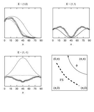
FIG. 1.: ARPES intensity at the Fermi energy (in arbitrary units) versus Fermi surface angle $\Phi$ (see lower right figure), for three different polarization directions. The curves were computed from the tight-binding model (solid line) and ZRS (dashed line). The photon energy is $h\nu=22\;eV$ and the curves are normalized to $\Phi=0$ in panel the upper left panel. The points represent the integrated intensities from first the first principle calculation of Bansil and Lindroos [17]. The lower right panel shows the geometrical details.

For an electron energy of $\approx 20\;eV$ the detector would have to be placed at $\approx 20^{o}$ degrees from the surface normal (neglecting the refraction by the potential step at the surface), and the $d_{x^{2}-y^{2}}$ orbital emits practically no electrons into this direction.
Next we note that light polarized along the $(1,0)$direction can only excite electrons from $p_{x}$-type orbitals, light polarized along the $(1,1)$ direction will excite the combination $p_{x}+p_{y}$, whereas light polarized along $(1,-1)$ excites $p_{x}-p_{y}$. Finally one has to bear in mind that near $(\pi,0)$ the tight-binding wave function contains only $p_{x}$-type orbitals (the mixing between $p_{y}(\pi,0)$ and $d_{x^{2}-y^{2}}(\pi,0)$ being exactly zero). Therefore the polarizations $(1,1)$ and $(1,-1)$ have equal intensity, whereas $(1,0)$ gives maximum intensity. Near $(0,\pi)$ in the other hand, the tight-binding wave function contains only $p_{y}$, whence the polarizations $(1,1)$ and $(1,-1)$ again have equal intensity, whereas $(1,0)$ this time gives no intensity. For $\mathchoice{{\hbox{\boldmath$\displaystyle k$}}}{{\hbox{\boldmath$\textstyle k$}}}{{\hbox{\boldmath$\scriptstyle k$}}}{{\hbox{\boldmath$\scriptscriptstyle k$}}}\;{\|}\;(1,1)$ exciting $p_{x}+p_{y}$ gives no intensity, because this combination does not mix with $d_{x^{2}-y^{2}}$ and hence is not contained in the tight-binding wave function, whereas exciting $p_{x}-p_{y}$ gives high intensity. The intensity for polarization $(1,0)$ at these momenta is approximately $1/2$ of that for $(\pi,0)$. These simple considerations obviously explain the overall shape of the curves in Figure 1 quite well. The main discrepancy between the Bansil-Lindroos theory and our calculation is the behaviour of the curve for polarization $(1,-1)$. Actually, this is the only curve which is not determined by symmetry alone, and subtle details of the wave function become important. We believe that the parameterization of Andersen et al. [16] does give the correct dispersion, but not necessarily the right wave functions. Next we consider the intensity variation along various high-symmetry lines in the Brillouin zone, shown in Figure 2.

FIG. 2.: Spectral weight along $(0,0)\rightarrow(\pi,0)$ and $(0,0)\rightarrow(\pi,\pi)$ compared to first principles calculation [17] (triangles). ZRS (solid line), tight-binding (long dashes) and CPT (short dashes) method show qualitatively good agreement. The strong decrease of the spectral weight in CPT towards $k=(\pi,0)$ may result from high doping ($\delta=25\%$).

FIG. 3.: Orbitals used for constructing a ZRS and signs of the different lobes.

Again, there is reasonable agreement between Bansil and Lindroos and our theory. All in all the comparison shows that also in the results of Bansil and Lindroos the behaviour of the intensity is to a considerable extent determined by the ‘radiation characteristics’ of the orbitals in the CuO₂ plane and the relative weight of the $p_{x}$ and $p_{y}$ orbitals. Additional complications like multiple scattering of the photoelectrons, Bragg scattering from the BiO surface layer etc. do not seem to have a very strong impact on the intensity variations, not even at the relatively low photon energy of $22\;eV$. Despite its simplicity we therefore believe that our theory has some merit, particularly so because it allows (unlike the single particle calculation of Bansil and Lindroos) to incorporate the effects of strong correlations. One weak point of all single-particle-like calculations for the CuO₂-plane is the following: since (in electron language) the band which forms the Fermi surface is the topmost one obtained by mixing the energetically higher Cu 3$d_{x^{2}-y^{2}}$-orbital with the energetically lower O 2p$\sigma$ orbitals it is clear, that the respective wave functions have predominant Cu 3$d_{x^{2}-y^{2}}$ character. This is exactly opposite to the actual situation in the cuprates, where the fist ionization states in the doped and undoped case are known to have predominant O 2p character. We now consider the case of large $U$. An exact calculation of the single-particle spectra (11) is no longer possible in this case and we have to use various approximations. First we study an isolated Zhang-Rice singlet (ZRS) in a single CuO₄ plaquette, see Figure 3. The bonding combination of $O$ $2p\sigma$-orbitals is

$\displaystyle p_{b,\sigma}^{\dagger}=\frac{1}{2}(p_{1,\sigma}^{\dagger}-p_{2,\sigma}^{\dagger}-p_{3,\sigma}^{\dagger}+p_{4,\sigma}^{\dagger})$

and the single-hole basis states (relevant at half-filling) can be written as

$$|1\rangle = p_{b,\sigma}|full\rangle,$$ (14)

$$|2\rangle = d_{\sigma}|full\rangle.$$ (15)

Here $|full\rangle$ denotes the $Cu3d^{10}\otimes 4\;O2p^{6}$ state. The single hole ground state then is $|\Psi_{0}^{(1h)}\rangle=\alpha|1\rangle+\beta|2\rangle$ where $(\alpha,\beta)$ is the normalized ground state eigenvector of the matrix

$$H=\left(\begin{array}[]{c c}0&2t_{pd}\\ 2t_{pd}&-\Delta\end{array}\right)$$ (16)

Two-hole states are obtained by starting from the basis states

$$|1^{\prime}\rangle = p_{b,\uparrow}p_{b,\downarrow}|full\rangle$$ (17)

$$|2^{\prime}\rangle = \frac{1}{\sqrt{2}}(p_{b,\uparrow}d_{\downarrow}+d_{\uparrow}p_{b,\downarrow})|full\rangle$$ (18)

$$|3^{\prime}\rangle = d_{\uparrow}d_{\downarrow}|full\rangle$$ (19)

The two-hole ground state of the plaquette reads $|\Psi_{0}^{(2h)}\rangle=\alpha^{\prime}|1^{\prime}\rangle+\beta^{\prime}|2^{\prime}\rangle+\gamma^{\prime}|3^{\prime}\rangle$, where $(\alpha^{\prime},\beta^{\prime},\gamma^{\prime})$ is an eigenvector of

$$H=\left(\begin{array}[]{c c c}0&2\sqrt{2}t_{pd}&0\\ 2\sqrt{2}t_{pd}&-\Delta&2\sqrt{2}t_{pd}\\ 0&2\sqrt{2}t_{pd}&-2\Delta+U\end{array}\right).$$ (20)

If we want to make contact with the $t-J$ model, where a ‘hole’ at site $i$ stands for a ZRS in the plaquette centered on the copper site $i$, we have to incorporate a phase factor of $e^{-i\mathchoice{{\hbox{\boldmath$\displaystyle k$}}}{{\hbox{\boldmath$\textstyle k$}}}{{\hbox{\boldmath$\scriptstyle k$}}}{{\hbox{\boldmath$\scriptscriptstyle k$}}}_{\|}\cdot\mathchoice{{\hbox{\boldmath$\displaystyle R$}}}{{\hbox{\boldmath$\textstyle R$}}}{{\hbox{\boldmath$\scriptstyle R$}}}{{\hbox{\boldmath$\scriptscriptstyle R$}}}_{i}}$, into the definition of $|\Psi_{0}^{(2h)}\rangle$, where $\mathchoice{{\hbox{\boldmath$\displaystyle R$}}}{{\hbox{\boldmath$\textstyle R$}}}{{\hbox{\boldmath$\scriptstyle R$}}}{{\hbox{\boldmath$\scriptscriptstyle R$}}}_{i}$ is the position of the central Cu orbital. In other words, the matrix element for the creation of a ‘hole’ in the $t-J$ model is

$$m_{ZRS}=e^{i\mathchoice{{\hbox{\boldmath$\displaystyle k$}}}{{\hbox{\boldmath$\textstyle k$}}}{{\hbox{\boldmath$\scriptstyle k$}}}{{\hbox{\boldmath$\scriptscriptstyle k$}}}_{\|}\cdot\mathchoice{{\hbox{\boldmath$\displaystyle R$}}}{{\hbox{\boldmath$\textstyle R$}}}{{\hbox{\boldmath$\scriptstyle R$}}}{{\hbox{\boldmath$\scriptscriptstyle R$}}}_{i}}\langle\Psi_{0}^{(2h)}|\tilde{c}_{\mathchoice{{\hbox{\boldmath$\displaystyle k$}}}{{\hbox{\boldmath$\textstyle k$}}}{{\hbox{\boldmath$\scriptstyle k$}}}{{\hbox{\boldmath$\scriptscriptstyle k$}}},\sigma}|\Psi_{0}^{(1h)}\rangle.$$ (21)

The matrix elements for the creation of $e^{-i\mathchoice{{\hbox{\boldmath$\displaystyle k$}}}{{\hbox{\boldmath$\textstyle k$}}}{{\hbox{\boldmath$\scriptstyle k$}}}{{\hbox{\boldmath$\scriptscriptstyle k$}}}_{\|}\cdot\mathchoice{{\hbox{\boldmath$\displaystyle R$}}}{{\hbox{\boldmath$\textstyle R$}}}{{\hbox{\boldmath$\scriptstyle R$}}}{{\hbox{\boldmath$\scriptscriptstyle R$}}}_{j}}p_{b,\sigma}|full\rangle$ and $e^{-i\mathchoice{{\hbox{\boldmath$\displaystyle k$}}}{{\hbox{\boldmath$\textstyle k$}}}{{\hbox{\boldmath$\scriptstyle k$}}}{{\hbox{\boldmath$\scriptscriptstyle k$}}}_{\|}\cdot\mathchoice{{\hbox{\boldmath$\displaystyle R$}}}{{\hbox{\boldmath$\textstyle R$}}}{{\hbox{\boldmath$\scriptstyle R$}}}{{\hbox{\boldmath$\scriptscriptstyle R$}}}_{j}}d_{\sigma}|full\rangle$ are

$$m_{b} = i\left(\mathchoice{{\hbox{\boldmath$\displaystyle v$}}}{{\hbox{\boldmath$\textstyle v$}}}{{\hbox{\boldmath$\scriptstyle v$}}}{{\hbox{\boldmath$\scriptscriptstyle v$}}}(p_{y})\sin(\frac{k_{y}}{2})-\mathchoice{{\hbox{\boldmath$\displaystyle v$}}}{{\hbox{\boldmath$\textstyle v$}}}{{\hbox{\boldmath$\scriptstyle v$}}}{{\hbox{\boldmath$\scriptscriptstyle v$}}}(p_{x})\sin(\frac{k_{x}}{2})\right)\cdot\mathchoice{{\hbox{\boldmath$\displaystyle\epsilon$}}}{{\hbox{\boldmath$\textstyle\epsilon$}}}{{\hbox{\boldmath$\scriptstyle\epsilon$}}}{{\hbox{\boldmath$\scriptscriptstyle\epsilon$}}},$$ (22)

$$m_{d} = \mathchoice{{\hbox{\boldmath$\displaystyle v$}}}{{\hbox{\boldmath$\textstyle v$}}}{{\hbox{\boldmath$\scriptstyle v$}}}{{\hbox{\boldmath$\scriptscriptstyle v$}}}(d_{x^{2}-y^{2}})\cdot\mathchoice{{\hbox{\boldmath$\displaystyle\epsilon$}}}{{\hbox{\boldmath$\textstyle\epsilon$}}}{{\hbox{\boldmath$\scriptstyle\epsilon$}}}{{\hbox{\boldmath$\scriptscriptstyle\epsilon$}}}.$$ (23)

Finally, the matrix element for creation of a ZRS from the single-hole ground state becomes

$$m_{ZRS} = \alpha^{\prime*}\alpha m_{b}+\frac{\beta^{\prime*}}{\sqrt{2}}(\alpha m_{d}+\beta m_{b})$$

$$+\gamma^{\prime*}\beta m_{d}.$$

Using this expression, the intensity expected for a ZRS with momentum $\textstyle k$ can be calculated as a function of photon polarization and energy. This will be discussed in the next sections.

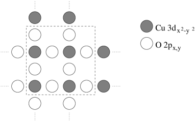
FIG. 4.: Three band Hubbard cluster used in the Lanczos diagonalization. The hopping across the cluster boundary (dashed line) is treated to lowest order strong coupling perturbation theory.

In comparing the intensities calculated from our above theory for a single ZRS to experiment one would be implicitly assuming that the first ionization states can be described completely by a coherent superposition of ZRS in a single plaquette. This need not be the case and in order to get at least a rough feeling for the effects of ‘embedding the plaquette in a lattice’ we use the technique of cluster perturbation theory (CPT) to study the extended system. CPT, which was first suggested by Senechal et al.[18], is a technique to ‘extrapolate’ the single-electron’s Green’s function calculated on a finite cluster to an infinite periodic system. It is based on an perturbative treatment of the intercluster hopping. The cluster we used for the present calculation is a quadratic arrangement of four unit cells each containing one Cu d${}_{x^{2}-y^{2}}$ and two O p_x,y orbitals as shown in figure 4. The Green’s function

$\displaystyle G_{ij\sigma}=\left<\Phi_{0}\right|c_{i\sigma}\frac{1}{z-H}c^{\dagger}_{j\sigma}\left|\Phi_{0}\right>+\left<\Phi_{0}\right|c^{\dagger}_{j\sigma}\frac{1}{z-H}c_{i\sigma}\left|\Phi_{0}\right>$

of this cluster with open boundary conditions is calculated by the Lanczos method. The boundary orbitals of the cluster are connected to the adjacent cluster by the Fourier transform of the intercluster hopping $V({\bf Q})$, where ${\bf Q}$ is a “superlattice” wave-vector restricted to the smaller Brillouin zone formed by the now enlarged lattice of the clusters. The perturbative treatment of the intercluster hopping in lowest order yields an RPA like expression for the approximate Green’s function.

$\displaystyle{\cal G}_{ij\sigma}\left({\bf Q},\omega\right)=\left(\frac{1}{G^{-1}(\omega)_{\sigma}-V({\bf Q})}\right)_{ij}.$

This mixed representation can then be transformed into momentum space by a Fourier transformation thereby taking into account the geometry of the cluster:

$\displaystyle G_{CPT}\left({\bf k},\omega\right)=\frac{1}{N}\sum_{ij}e^{i{\bf k}\left({\bf r}_{i}-{\bf r}_{j}\right)}{\cal G}_{ij\sigma}\left({\bf N}{\bf k},\omega\right).$

This result is exact for $U=0$ and has been shown[18] to produce good results also for large and intermediate $U$. In the following sections we will use this technique for the approximate calculation of the single-particle spectral densities as a valuable cross-check for the calculations based on a single ZRS. While CPT still is far from being rigorous, it includes some effects which result from embedding the ZRS in a lattice and, as we will in fact see, it always gives results which are very similar to those for a ZRS.
To conclude this section we want to give a simple estimate for the photoelectron kinetic energy $T$ as a function of photon energy $h\nu$. It is easy to see that in the absence of any potential step at the surface of the solid we would have

$$T=h\nu+E_{0}^{(N)}-E_{\mathchoice{{\hbox{\boldmath$\displaystyle k$}}}{{\hbox{\boldmath$\textstyle k$}}}{{\hbox{\boldmath$\scriptstyle k$}}}{{\hbox{\boldmath$\scriptscriptstyle k$}}}}^{(N-1)}$$ (24)

where $E_{0}^{(N)}$ is the energy of the ground state of the solid with $N$ electrons and $E_{\mathchoice{{\hbox{\boldmath$\displaystyle k$}}}{{\hbox{\boldmath$\textstyle k$}}}{{\hbox{\boldmath$\scriptstyle k$}}}{{\hbox{\boldmath$\scriptscriptstyle k$}}}}^{(N-1)}$ the final state of the solid. We approximate

$$E_{0}^{(N)}-E_{\mathchoice{{\hbox{\boldmath$\displaystyle k$}}}{{\hbox{\boldmath$\textstyle k$}}}{{\hbox{\boldmath$\scriptstyle k$}}}{{\hbox{\boldmath$\scriptscriptstyle k$}}}}^{(N-1)}\approx(E_{0}^{1h}-E_{0}^{2h})-E_{2p}$$ (25)

Here $E_{0}^{nh}$ are the ground state energies of a CuO₄ plaquette with $n$ holes, obtained by diagonalizing the matrices (16) and (20). In these matrices the energy of the $O2p$ level, $E_{2p}$, has been chosen as the zero of energy, whence it has to be taken into account separately. For the ‘standard values’ of the parameters $t_{pd}=-1.3\;eV$, $\Delta=3.6\;eV$ and $U=10.5\;eV$ this gives $E_{0}^{1h}-E_{0}^{2h}=1.93\;eV$. Using the estimate $E_{2p}\approx-10\;eV$ from our atomic LDA calculation we find

$$T\approx h\nu-8\;eV,$$ (26)

which we will use in all that follows.

FIG. 5.: Spectral weight along $(0,0)\rightarrow(\pi,0)$ and $(0,0)\rightarrow(\pi,\pi)$ compared to experimental data from references [17, 6].

As a first application, Figure 5 then shows the intensity of the topmost ARPES peak calculated by CPT and compares this to experimental data. Reasonable qualitative agreement can be found, especially for the CPT calculation, although the shift of the spectral weight maximum towards $k=(\pi,0)$ for $22\;eV$ is not reproduced. The much better agreement for $E_{photon}=34eV$ suggests that for the lower photon energy of $22\;eV$ additional effects (such as multiple scattering corrections or Bragg-scattering from the BiO top-layer) are more important.

IV Application to experiment

Coming back to the theory for the ZRS we can already draw conclusions of some importance. By combining the expressions for the vectors $\mathchoice{{\hbox{\boldmath$\displaystyle v$}}}{{\hbox{\boldmath$\textstyle v$}}}{{\hbox{\boldmath$\scriptstyle v$}}}{{\hbox{\boldmath$\scriptscriptstyle v$}}}_{l,\alpha}$ from Appendix II with the ‘form factor’ of a ZRS, (23), the expression for the photocurrent can be brought to the form

$$\mathchoice{{\hbox{\boldmath$\displaystyle j$}}}{{\hbox{\boldmath$\textstyle j$}}}{{\hbox{\boldmath$\scriptstyle j$}}}{{\hbox{\boldmath$\scriptscriptstyle j$}}}\propto|\sum_{l,l^{\prime}}\tilde{R}_{l,l^{\prime}}(E)\;(\mathchoice{{\hbox{\boldmath$\displaystyle v$}}}{{\hbox{\boldmath$\textstyle v$}}}{{\hbox{\boldmath$\scriptstyle v$}}}{{\hbox{\boldmath$\scriptscriptstyle v$}}}_{l,l^{\prime}}(\mathchoice{{\hbox{\boldmath$\displaystyle k$}}}{{\hbox{\boldmath$\textstyle k$}}}{{\hbox{\boldmath$\scriptstyle k$}}}{{\hbox{\boldmath$\scriptscriptstyle k$}}}_{\|},\mathchoice{{\hbox{\boldmath$\displaystyle k$}}}{{\hbox{\boldmath$\textstyle k$}}}{{\hbox{\boldmath$\scriptstyle k$}}}{{\hbox{\boldmath$\scriptscriptstyle k$}}})\cdot{\bf\epsilon})\;|^{2}.$$ (27)

We remember that $\mathchoice{{\hbox{\boldmath$\displaystyle k$}}}{{\hbox{\boldmath$\textstyle k$}}}{{\hbox{\boldmath$\scriptstyle k$}}}{{\hbox{\boldmath$\scriptscriptstyle k$}}}_{\|}$ is the momentum of the photohole (which is within the first Brillouin zone of the CuO₂ plane), whereas $\textstyle k$ is the momentum of the escaping photoelectron. Using the expressions from Appendix II it is now a matter of straightforward algebra to derive the following expressions for $\mathchoice{{\hbox{\boldmath$\displaystyle k$}}}{{\hbox{\boldmath$\textstyle k$}}}{{\hbox{\boldmath$\scriptstyle k$}}}{{\hbox{\boldmath$\scriptscriptstyle k$}}}_{\|}=(k,0)$, and the ‘optimal’ photon polarization for momenta along $(1,0)$, $\mathchoice{{\hbox{\boldmath$\displaystyle\epsilon$}}}{{\hbox{\boldmath$\textstyle\epsilon$}}}{{\hbox{\boldmath$\scriptstyle\epsilon$}}}{{\hbox{\boldmath$\scriptscriptstyle\epsilon$}}}=(1,0,0)$:

$$\mathchoice{{\hbox{\boldmath$\displaystyle v$}}}{{\hbox{\boldmath$\textstyle v$}}}{{\hbox{\boldmath$\scriptstyle v$}}}{{\hbox{\boldmath$\scriptscriptstyle v$}}}_{0,1}\cdot\mathchoice{{\hbox{\boldmath$\displaystyle\epsilon$}}}{{\hbox{\boldmath$\textstyle\epsilon$}}}{{\hbox{\boldmath$\scriptstyle\epsilon$}}}{{\hbox{\boldmath$\scriptscriptstyle\epsilon$}}} = \frac{\sin(k/2)}{\sqrt{12\pi}},$$ (28)

$$\mathchoice{{\hbox{\boldmath$\displaystyle v$}}}{{\hbox{\boldmath$\textstyle v$}}}{{\hbox{\boldmath$\scriptstyle v$}}}{{\hbox{\boldmath$\scriptscriptstyle v$}}}_{1,2}\cdot\mathchoice{{\hbox{\boldmath$\displaystyle\epsilon$}}}{{\hbox{\boldmath$\textstyle\epsilon$}}}{{\hbox{\boldmath$\scriptstyle\epsilon$}}}{{\hbox{\boldmath$\scriptscriptstyle\epsilon$}}} = -i\sqrt{\frac{3}{20\pi}}\;\sin(\Theta),$$ (29)

$$\mathchoice{{\hbox{\boldmath$\displaystyle v$}}}{{\hbox{\boldmath$\textstyle v$}}}{{\hbox{\boldmath$\scriptstyle v$}}}{{\hbox{\boldmath$\scriptscriptstyle v$}}}_{2,1}\cdot\mathchoice{{\hbox{\boldmath$\displaystyle\epsilon$}}}{{\hbox{\boldmath$\textstyle\epsilon$}}}{{\hbox{\boldmath$\scriptstyle\epsilon$}}}{{\hbox{\boldmath$\scriptscriptstyle\epsilon$}}} = \frac{\sin(k/2)}{\sqrt{12\pi}}\left(\frac{3}{2}\cos(2\Theta)-\frac{1}{2}\right),$$ (30)

$$\mathchoice{{\hbox{\boldmath$\displaystyle v$}}}{{\hbox{\boldmath$\textstyle v$}}}{{\hbox{\boldmath$\scriptstyle v$}}}{{\hbox{\boldmath$\scriptscriptstyle v$}}}_{3,2}\cdot\mathchoice{{\hbox{\boldmath$\displaystyle\epsilon$}}}{{\hbox{\boldmath$\textstyle\epsilon$}}}{{\hbox{\boldmath$\scriptstyle\epsilon$}}}{{\hbox{\boldmath$\scriptscriptstyle\epsilon$}}} = -i\sqrt{\frac{3}{20\pi}}\;\sin(\Theta)\;(\frac{5}{4}\cos(2\Theta)-\frac{1}{4}).$$ (31)

Figure 6 shows the $\Theta$-dependence of these expressions.

FIG. 6.: ‘Radiation characteristics’ $|\mathchoice{{\hbox{\boldmath$\displaystyle v$}}}{{\hbox{\boldmath$\textstyle v$}}}{{\hbox{\boldmath$\scriptstyle v$}}}{{\hbox{\boldmath$\scriptscriptstyle v$}}}_{l,l^{\prime}}\cdot\mathchoice{{\hbox{\boldmath$\displaystyle\epsilon$}}}{{\hbox{\boldmath$\textstyle\epsilon$}}}{{\hbox{\boldmath$\scriptstyle\epsilon$}}}{{\hbox{\boldmath$\scriptscriptstyle\epsilon$}}}|^{2}$ for the different partial waves from a ZRS with momentum $(\pi,0)$. The figure shows the $\Theta$-dependence of the respective partial wave within in the $x-z$ plane. The polarization vector $\textstyle\epsilon$ of the exciting light is assumed to be in $x$-direction.

Obviously a ZRS with momentum near $(\pi,0)$ emits photoelectrons predominantly parallel to the CuO₂ plane if it is excited with light polarized along $(1,0)$ within the CuO₂ plane. The situation is similar, though not as pronounced, for other momenta, such as $(\frac{\pi}{2},\frac{\pi}{2})$. It should be noted, that the vectors $\mathchoice{{\hbox{\boldmath$\displaystyle v$}}}{{\hbox{\boldmath$\textstyle v$}}}{{\hbox{\boldmath$\scriptstyle v$}}}{{\hbox{\boldmath$\scriptscriptstyle v$}}}_{l,l^{\prime}}(\mathchoice{{\hbox{\boldmath$\displaystyle k$}}}{{\hbox{\boldmath$\textstyle k$}}}{{\hbox{\boldmath$\scriptstyle k$}}}{{\hbox{\boldmath$\scriptscriptstyle k$}}}_{\|},\mathchoice{{\hbox{\boldmath$\displaystyle k$}}}{{\hbox{\boldmath$\textstyle k$}}}{{\hbox{\boldmath$\scriptstyle k$}}}{{\hbox{\boldmath$\scriptscriptstyle k$}}})$ are computed exactly namely by elementary angular-momentum recoupling. The fact that a ZRS with momentum near $(\pi,0)$ emits photoelectrons predominantly at small angles with respect to the CuO₂ plane therefore is a rigorous result.
The radial matrix elements $\tilde{R}_{l,l^{\prime}}(E)$ which also enter in (27) actually tend to suppress the emission close to the surface normal even more. Namely one finds (Appendix I) that $R_{0,1}\approx 0.2\;R_{2,1}$, that means the $s$-like partial wave (which would contribute strongly to emission at near perpendicular directions, see Figure 6) has a very small weight due to the radial matrix elements. We note in passing that the smallness of the ratio $R_{0,1}/R_{2,1}$ is well-known in the EXAFS literature[19].
Combining the partial waves in Figure 6 with the proper radial matrix elements $\tilde{R}_{l,l^{\prime}}(E)$ as in (27) we expect to obtain a curve with a minimum for some finite $\Theta$ (mainly due to to the node in the dominant $d$-like $l=2$ partial wave emitted by the 2p $l^{\prime}=1$ orbital (see Figure 6). This may in fact explain a well-known[7] effect in ARPES, namely the the relatively strong asymmetry with respect to $(\pi,0)$ of the ARPES intensity for $\mathchoice{{\hbox{\boldmath$\displaystyle k$}}}{{\hbox{\boldmath$\textstyle k$}}}{{\hbox{\boldmath$\scriptstyle k$}}}{{\hbox{\boldmath$\scriptscriptstyle k$}}}_{\|}$ along $(1,0)$ which

FIG. 7.: ARPES intensity as a function of momentum along $(1,0)$ for different photon energies, calculated by for an isolated ZRS. The inset shows the radiation characteristics of a ZRS at $(\pi,0)$ and the directions at which a detector would have to be placed at photon energy $22\;eV$ to observe the respective momentum. Thereby the work function is neglected.

is seen at $22\;eV$ photon energy but not at $34\;eV$. Figure 7 shows the calculated intensities as a function of in-plane momentum. For $h\nu\approx 22\;eV$ the angles$\Theta$ which would be appropriate to observe $\mathchoice{{\hbox{\boldmath$\displaystyle k$}}}{{\hbox{\boldmath$\textstyle k$}}}{{\hbox{\boldmath$\scriptstyle k$}}}{{\hbox{\boldmath$\scriptscriptstyle k$}}}_{\|}$ slightly beyond $(\pi,0)$ (i.e. in the second zone) are such, that one is ‘looking into the node’ of the radiation characteristics of the ZRS, whereas for smaller $\mathchoice{{\hbox{\boldmath$\displaystyle k$}}}{{\hbox{\boldmath$\textstyle k$}}}{{\hbox{\boldmath$\scriptstyle k$}}}{{\hbox{\boldmath$\scriptscriptstyle k$}}}_{\|}$ one is looking at the maximum (see the inset). Hence there is a strong asymmetry around $(\pi,0)$. Increasing the energy to $\geq 30eV$ the angles $\Theta$ becomes smaller, one is no longer sampling the node and the the intensity is much more symmetric around $(\pi,0)$.
As shown in the preceding discussion, our theory reproduced, despite its simplicity, some experimental features seen in the cuprates. We therefore proceed to address potential applications in experiment. Thereby the main goal is to find experimental conditions under which the ZRS-derived state at a given momentum ${\bf k}_{\|}$ can be observed with the highest intensity. To that end, we can vary different experimental parameters, mainly the direction of the photon polarization and the Brillouin zone in which we are measuring.
We first consider the case of normal incidence of the light, that means the electric field vector $\textstyle\epsilon$ is in the CuO₂ plane. Rotating $\textstyle\epsilon$ in the plane will change the intensity from the ZRS-derived states in a systematic way, and for some angle $\Phi_{E}$ it will be maximum. Along high symmetry directions like $(1,1)$ or $(1,0)$ the optimal polarization can be deduced by symmetry considerations, because the ZRS has a definite parity under reflections by these directions. For momenta $\textstyle k$ along $(1,1)$ $\textstyle\epsilon$ has to be perpendicular to $\textstyle k$, whereas along $(1,0)$ it must be parallel[1]. For nonsymmetric momenta, however, this symmetry analysis is not possible and one has to calculate the optimum direction. We note that apart from merely enhancing the intensity of the ZRS, knowledge of the polarization dependence of the ARPES intensity of the ‘ideal’ ZRS would allow also to separate the original signal from ZRS-derived states from any ‘background’, that means photoelectrons which have undergone inelastic scattering on their way to the analyzer. Since it is plausible that these background electrons have more or less lost the information about the polarization of the incoming light, their contribution should be insensitive to polarization. Taking the spectrum at the ‘optimal angle’ for the ZRS and perpendicular to it then would allow to remove the background by merely subtracting the two spectra (provided one can measure the absolute intensity). Along the high symmetry directions $(1,0)$ and $(1,1)$ the feasibility of this procedure has recently been demonstrated by Manzke et al. [20] and using the calculated optimal polarizations this analysis could be extended to any point in the BZ.
For the special case of the ZRS, and neglecting the contribution of copper altogether, it is possible to give a rather simple expression for the optimal angle. The matrix element for creating the bonding combination of O 2p$\sigma$ orbitals is

$$m_{ZRS} \propto i\left(\sin(\Phi_{E})\sin(\frac{k_{y}}{2})-\cos(\Phi_{E})\sin(\frac{k_{x}}{2})\right).$$ (32)

We thus find the angles which give minimum and maximum intensity:

$$\sin(\Phi_{E,min})\sin(\frac{k_{y}}{2})-\cos(\Phi_{\min})\sin(\frac{k_{x}}{2}) = 0$$ (33)

$$\cos(\Phi_{E,max})\sin(\frac{k_{y}}{2})+\sin(\Phi_{\max})\sin(\frac{k_{x}}{2}) = 0$$ (34)

We see that always $\Phi_{E,min}=\Phi_{E,max}+\frac{\pi}{2}$. Moreover, in this approximation the intensity is exactly zero for $\Phi_{E,min}$, and the angle for maximum intensity is

$$\Phi_{E,max}=-arctan\left(\frac{\sin(\frac{k_{y}}{2})}{\sin(\frac{k_{x}}{2})}\right).$$ (35)

This expression takes a particularly simple form along the line $(\pi,0)\rightarrow(0,\pi)$, where $\Phi_{\max}=-k_{y}/2$. This reproduces the known values $\Phi_{\max}=0$ along $(1,0)$, $\Phi_{\max}=-\frac{\pi}{4}$ along $(1,1)$ and $\Phi_{\max}=-\frac{\pi}{2}$ along $(0,1)$. Despite its simplicity formula (35) gives a quite good estimate for the optimum polarization. Numerical evaluation shows that the lines of constant $\Phi_{\max}$ in $\textstyle k$-space are to very good approximation straight lines through the center of the Brillouin zone. This means that in practice one could adjust the polarization angle $\Phi_{E}$ once to either $\Phi_{E,max}$ or $\Phi_{E,min}$, and then scan an entire straight line through the origin by varying the emission angle $\Theta_{k}$ without having to change the polarization along the way.

FIG. 8.: Optimal in-plane polarization for observing the ZRS at the respective position in the Brillouin zone by ARPES with photoelectron kinetic energy energy. The calculation is done for an isolated ZRS.

Figures 8 and 9 then show the optimal angle for observation of the first ionization state for momenta in the first Brillouin zone. For perpendicular polarization the intensity practically vanishes. In the Figure we compare the ‘isolated ZRS’ and the ‘embedded ZRS’ whose spectra are obtained by CPT. Both methods of calculation give very similar results for the optimal angle, which in turn agrees very well with the simple estimate 35. Since along the high symmetry lines $(1,0)$ and $(1,1)$ the optimal $\Phi_{E}$ is determined by symmetry alone there is obviously not so much freedom to ‘interpolate’ smoothly between these values.
Next, moving to a higher Brillouin zone allows to enhance the intensity of the ZRS, as can be seen from Table I and II. Table I shows the ratio $I/I_{0}$ of the intensity obtainable by measuring the ZRS at $(\frac{\pi}{2},\frac{\pi}{2})$ at the ‘original position’ (there the polarization has to be perpendicular to (1,1) by symmetry) and the intensity that can be obtained by measuring in a higher zone with optimized polarization, both within in the CuO₂ plane and, for later reference, also out of plane.

FIG. 9.: Optimal in-plane polarization for observing the first ionization state of the correlated CuO₂ plane. The intensities are calculated by integrating the spectral weight obtained by CPT within 300meV.

The same information is given for $(\pi,0)$ in table II. Obviously, an enhancement of a factor of $2$ or more can be achieved by proper choice of the experimental conditions. In view of the large ‘background’ in the experimental spectra, even such a moderate enhancement may be quite important.
We note that the physical origin of the variation of intensity with $\Phi_{E}$ and order of the Brillouin zone

FIG. 10.: ‘Radiation characteristics’ within the $(x-z)$ plane of a ZRS excited with light polarized in the $(x-z)$ plane. The polar angles are $\Theta_{E}=\frac{\pi}{2}$ (dashed line) and $\Theta_{E}=\Theta_{E,opt}\approx\frac{\pi}{3}$ (full line). The skew line shows the direction where the detector would have to be placed for the photon energy of $22\;eV$ (work function neglected).

is the interference between the processes of creating a photohole in $p_{x}$-like and $p_{y}$-like $O$ $2p\sigma$ orbitals. By changing $\Phi_{E}$ the relative intensity and phase between photoholes in the two types of orbitals can be tuned. Thus, one can always find an angle $\Phi_{E,max}$ where the interference between these two types of orbital is maximally constructive. This angle depends on the relative phase between the two orbitals in the wave function and thus is specific for the state in question. Next, we study a quite different effect, namely what happens if we tilt the polarization vector $\textstyle\epsilon$ out of the CuO₂ plane. To illustrate the usefulness of this, we again consider a momentum along the high symmetry line $(0,0)\rightarrow(\pi,0)$ and assume that the polarization vector $\textstyle\epsilon$ is within in $x-z$ plane It follows from symmetry considerations that any component of the light perpendicular to this plane (‘s-polarization’) cannot excite any ZRS-derived states. In other words we assume that $\Phi_{E}$ but that $\Theta_{E}$ is variable. The contribution from the bonding combination of $O$ $2p\sigma$ orbitals then becomes

$$m_{ZRS} = -i\xi_{1}\Bigg{[}\left(\frac{1}{\sqrt{3}}\tilde{R}_{01}s+\frac{1}{\sqrt{15}}\tilde{R}_{21}d_{3z^{2}-r^{2}}-\frac{1}{\sqrt{5}}\tilde{R}_{21}d_{x^{2}-y^{2}}\right)\sin(\Theta)+\frac{1}{\sqrt{5}}\tilde{R}_{21}d_{xz}\cos(\Theta)\Bigg{]}$$

$$+i\xi_{2}\Bigg{[}\left(-\frac{1}{\sqrt{5}}\tilde{R}_{321}p_{x}-\frac{1}{\sqrt{70}}\tilde{R}_{323}f_{x\left(5z^{2}-1\right)}+\sqrt{\frac{3}{70}}\tilde{R}_{323}f_{x^{3}-3xy^{2}}\right)\sin(\Theta)+\frac{1}{\sqrt{7}}\tilde{R}_{323}f_{z\left(x^{2}-y^{2}\right)}\cos(\Theta)\Bigg{]},$$

where $\xi_{1}=\alpha^{\prime*}\alpha+\frac{\beta^{\prime*}\beta}{\sqrt{2}}$ and $\xi_{2}=\gamma^{\prime*}\beta+\frac{\beta^{\prime*}\alpha}{\sqrt{2}}$. Tilting the electric field vector out of the plane thus admixes the $d_{xz}$ harmonic into the radiation characteristics, which has its maximum intensity at an angle of $45^{o}$ with respect to the CuO₂ plane. Clearly, this enhances the intensity at intermediate $\Theta_{k}$, particularly so if constructive interference with the $d_{x^{2}-y^{2}}$ and $d_{3z^{2}-r^{2}}$ harmonics (which are excited by the $x$-component of $\textstyle\epsilon$) occurs. Since the $d_{xz}$ on one hand and the $d_{x^{2}-y^{2}}$ and $d_{3z^{2}-r^{2}}$ on the other have opposite parity under reflection by the $y-z$ plane, constructive interference for some momentum $(k,0)$ automatically implies destructive interference for momentum $(-k,0)$. Tilting the electric field out of the plane thus amounts to ‘focusing’ the photoelectrons towards the detector. This effect is illustrated in Figure 10, which shows the angular variation within the $(x-z)$ plane of the photocurrent radiated by a ZRS.

FIG. 11.: Intensity of ZRS derived states with different momenta along the $(1,0)$-direction, as a function of the polar angle $\Theta_{E}$. The light is polarized in the $(x-z)$ plane, i.e. $\Phi_{E}=0$, the photon energy is $22\;eV$ (work function neglected).

Figure 11 then shows the intensity as a function of $\Theta_{E}$ for various momenta along $(0,0)\rightarrow(\pi,0)$. Remarkably enough, the enhancement of current towards the detector may be up to a factor of $3$ as compared to polarization in the plane. Exploiting this effect could enhance the photoemission intensity considerably in the region around $(\pi,0)$ - which might be important, because this is precisely the ‘controversial’ region in $\textstyle k$-space which makes the difference between hole-like[1, 4, 5, 6] and electron-like[7, 8, 9, 10] Fermi surface in Bi2212 and where bilayer-splitting[21, 22] should be observable. One caveat is the fact, that for a polarization which is not in the plane one has to compute the actual field direction by use of the Fresnel formulae[23]. The value of the dielectric constant, however, which has to be chosen for such a calculation, is very close to $1$. Tables I and II also give the optimal angles $\Theta_{E}$ and $\Phi_{E}$ for observing $(\frac{\pi}{2},\frac{\pi}{2})$ and $(\pi,0)$ in higher Brillouin zones. Obviously, by choosing the right zone and the right polarization a considerable enhancement of the intensity can be achieved.

V Surface resonances and the energy dependence of the intensity

We have seen in the preceding sections that the orbitals from which the ZRS is built emit photoelectrons predominantly at grazing angles with respect to the CuO₂ plane (see Figure 6). In most cases electrons emitted with momentum $(\mathchoice{{\hbox{\boldmath$\displaystyle k$}}}{{\hbox{\boldmath$\textstyle k$}}}{{\hbox{\boldmath$\scriptstyle k$}}}{{\hbox{\boldmath$\scriptscriptstyle k$}}}_{\|}+\mathchoice{{\hbox{\boldmath$\displaystyle G$}}}{{\hbox{\boldmath$\textstyle G$}}}{{\hbox{\boldmath$\scriptstyle G$}}}{{\hbox{\boldmath$\scriptscriptstyle G$}}}_{\|},k_{\perp}^{\prime})$ will be simply ‘lost’ because they will not reach a detector positioned to collect electrons with momentum $(\mathchoice{{\hbox{\boldmath$\displaystyle k$}}}{{\hbox{\boldmath$\textstyle k$}}}{{\hbox{\boldmath$\scriptstyle k$}}}{{\hbox{\boldmath$\scriptscriptstyle k$}}}_{\|},k_{\perp})$ (it might happen that the photoelectron ‘gets rid of its $\mathchoice{{\hbox{\boldmath$\displaystyle G$}}}{{\hbox{\boldmath$\textstyle G$}}}{{\hbox{\boldmath$\scriptstyle G$}}}{{\hbox{\boldmath$\scriptscriptstyle G$}}}_{\|}$’ by Bragg-scattering at the BiO surface layer - a possibility which we are neglecting here). It may happen, however, that the motion with momentum $\mathchoice{{\hbox{\boldmath$\displaystyle k$}}}{{\hbox{\boldmath$\textstyle k$}}}{{\hbox{\boldmath$\scriptstyle k$}}}{{\hbox{\boldmath$\scriptscriptstyle k$}}}_{\|}+\mathchoice{{\hbox{\boldmath$\displaystyle G$}}}{{\hbox{\boldmath$\textstyle G$}}}{{\hbox{\boldmath$\scriptstyle G$}}}{{\hbox{\boldmath$\scriptscriptstyle G$}}}_{\|}$ parallel to the surface ‘consumes so much energy’ that there is hardly any energy left for the motion perpendicular to the surface. This will happen whenever the kinetic energy $T$ is just above the so-called emergence condition for the reciprocal lattice vector $\mathchoice{{\hbox{\boldmath$\displaystyle G$}}}{{\hbox{\boldmath$\textstyle G$}}}{{\hbox{\boldmath$\scriptstyle G$}}}{{\hbox{\boldmath$\scriptscriptstyle G$}}}_{\|}$:

$$T=\frac{\hbar^{2}}{2m}(\mathchoice{{\hbox{\boldmath$\displaystyle k$}}}{{\hbox{\boldmath$\textstyle k$}}}{{\hbox{\boldmath$\scriptstyle k$}}}{{\hbox{\boldmath$\scriptscriptstyle k$}}}_{\|}+\mathchoice{{\hbox{\boldmath$\displaystyle G$}}}{{\hbox{\boldmath$\textstyle G$}}}{{\hbox{\boldmath$\scriptstyle G$}}}{{\hbox{\boldmath$\scriptscriptstyle G$}}}_{\|})^{2}.$$ (36)

In other words: the kinetic energy is ‘just about sufficient’ to create a free electron state with 3D momentum $(\mathchoice{{\hbox{\boldmath$\displaystyle k$}}}{{\hbox{\boldmath$\textstyle k$}}}{{\hbox{\boldmath$\scriptstyle k$}}}{{\hbox{\boldmath$\scriptscriptstyle k$}}}_{\|}+\mathchoice{{\hbox{\boldmath$\displaystyle G$}}}{{\hbox{\boldmath$\textstyle G$}}}{{\hbox{\boldmath$\scriptstyle G$}}}{{\hbox{\boldmath$\scriptscriptstyle G$}}},0)$. In this case the energy available for motion perpendicular to the surface is not sufficient for the photoelectron to surmount the energy barrier at the surface and it will be reflected back in to the solid.
On the other hand, if the ‘perpendicular energy’ is below the energy of the Hubbard gap as well, the electron cannot re-enter the solid either, because there are no single-particle states available in the solid with the proper energy. The situation thus is quite analogous to the case of the so-called Shockley state seen on the Cu surface: a combination of surface potential and a gap in the single-particle DOS causes the electron to be trapped at the surface of the solid. For an extensive review of the properties of such so-called surface resonances see Ref.[24].
The existence of such surface resonances also in a cuprate-related material has been established by Pothuizen[25]. In an extensive EELS study of Sr₂CuCl₂O₂, Pothuizen could in fact identify not just one, but a total of $3$ such states (in some cases with clearly resolved dispersion) in the energy window $0-30\;eV$. His results show very clearly that such surface states do exist in Sr₂CuCl₂O₂ - whether this holds true for other cuprate materials has not been established yet, but for the moment we will take their existence for granted.
To proceed in at least a semiquantitative way we use a very simple approximation[24]. We decompose the potential felt by an electron at the surface as

$$V(\mathchoice{{\hbox{\boldmath$\displaystyle r$}}}{{\hbox{\boldmath$\textstyle r$}}}{{\hbox{\boldmath$\scriptstyle r$}}}{{\hbox{\boldmath$\scriptscriptstyle r$}}}) = V_{av}(z)+V_{1}(\mathchoice{{\hbox{\boldmath$\displaystyle r$}}}{{\hbox{\boldmath$\textstyle r$}}}{{\hbox{\boldmath$\scriptstyle r$}}}{{\hbox{\boldmath$\scriptscriptstyle r$}}}),$$ (37)

$$V_{av}(z) = \frac{1}{a^{2}}\int_{0}^{a}dx\int_{0}^{a}dy\;V(x,y,z),$$ (38)

$$V_{1}(\mathchoice{{\hbox{\boldmath$\displaystyle r$}}}{{\hbox{\boldmath$\textstyle r$}}}{{\hbox{\boldmath$\scriptstyle r$}}}{{\hbox{\boldmath$\scriptscriptstyle r$}}}) = V(\mathchoice{{\hbox{\boldmath$\displaystyle r$}}}{{\hbox{\boldmath$\textstyle r$}}}{{\hbox{\boldmath$\scriptstyle r$}}}{{\hbox{\boldmath$\scriptscriptstyle r$}}})-V_{av}(z),$$ (39)

($a$ denotes the planar lattice constant) and assume that $V_{1}$ can be treated as a perturbation. The eigenstates of an electron in the potential $V_{av}(z)$ can be factorized:

$\displaystyle\Psi_{\mathchoice{{\hbox{\boldmath$\displaystyle G$}}}{{\hbox{\boldmath$\textstyle G$}}}{{\hbox{\boldmath$\scriptstyle G$}}}{{\hbox{\boldmath$\scriptscriptstyle G$}}}_{\|},\mu}(\mathchoice{{\hbox{\boldmath$\displaystyle r$}}}{{\hbox{\boldmath$\textstyle r$}}}{{\hbox{\boldmath$\scriptstyle r$}}}{{\hbox{\boldmath$\scriptscriptstyle r$}}})=e^{i(\mathchoice{{\hbox{\boldmath$\displaystyle k$}}}{{\hbox{\boldmath$\textstyle k$}}}{{\hbox{\boldmath$\scriptstyle k$}}}{{\hbox{\boldmath$\scriptscriptstyle k$}}}_{\|}+\mathchoice{{\hbox{\boldmath$\displaystyle G$}}}{{\hbox{\boldmath$\textstyle G$}}}{{\hbox{\boldmath$\scriptstyle G$}}}{{\hbox{\boldmath$\scriptscriptstyle G$}}}_{\|})\cdot\mathchoice{{\hbox{\boldmath$\displaystyle r$}}}{{\hbox{\boldmath$\textstyle r$}}}{{\hbox{\boldmath$\scriptstyle r$}}}{{\hbox{\boldmath$\scriptscriptstyle r$}}}}\;\Psi_{\mu}(z)$

with corresponding energy

$\displaystyle E(\mathchoice{{\hbox{\boldmath$\displaystyle G$}}}{{\hbox{\boldmath$\textstyle G$}}}{{\hbox{\boldmath$\scriptstyle G$}}}{{\hbox{\boldmath$\scriptscriptstyle G$}}}_{\|})=E_{\mu}+\frac{\hbar^{2}(\mathchoice{{\hbox{\boldmath$\displaystyle k$}}}{{\hbox{\boldmath$\textstyle k$}}}{{\hbox{\boldmath$\scriptstyle k$}}}{{\hbox{\boldmath$\scriptscriptstyle k$}}}_{\|}+\mathchoice{{\hbox{\boldmath$\displaystyle G$}}}{{\hbox{\boldmath$\textstyle G$}}}{{\hbox{\boldmath$\scriptstyle G$}}}{{\hbox{\boldmath$\scriptscriptstyle G$}}}_{\|})^{2}}{2m}.$

A surface resonance would correspond to a $\Psi_{\mu}(z)$ which is localized around the surface.
Let us now consider the subspace of eigenstates of $V_{av}(z)$ which comprises
a) the (discrete) surface resonance state $\Psi_{\mathchoice{{\hbox{\boldmath$\displaystyle G$}}}{{\hbox{\boldmath$\textstyle G$}}}{{\hbox{\boldmath$\scriptstyle G$}}}{{\hbox{\boldmath$\scriptscriptstyle G$}}}_{\|},\mu}$ and
b) the continuum of states $\Psi(\mathchoice{{\hbox{\boldmath$\displaystyle k$}}}{{\hbox{\boldmath$\textstyle k$}}}{{\hbox{\boldmath$\scriptstyle k$}}}{{\hbox{\boldmath$\scriptscriptstyle k$}}}_{\|},k_{\perp})$ which evolve into plane waves with momentum $(\mathchoice{{\hbox{\boldmath$\displaystyle k$}}}{{\hbox{\boldmath$\textstyle k$}}}{{\hbox{\boldmath$\scriptstyle k$}}}{{\hbox{\boldmath$\scriptscriptstyle k$}}}_{\|},k_{\perp})$ asymptotically far away from the surface. The periodic surface potential (i.e. the term $V_{1}$) then provides a mechanism for mixing $\Psi_{\mathchoice{{\hbox{\boldmath$\displaystyle G$}}}{{\hbox{\boldmath$\textstyle G$}}}{{\hbox{\boldmath$\scriptstyle G$}}}{{\hbox{\boldmath$\scriptscriptstyle G$}}}_{\|},\mu}$ and the continuum. Moreover, dipole transitions of an electron from the valence band into both a continuum state and into the surface resonance (whereby the latter alternative is possibly even more probable due to the special radiation characteristics of a ZRS) are possible. We thus have all ingredients for the standard Fano-type resonance (see Figure 12) and we would thus expect a pronounced peak

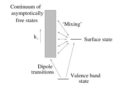
FIG. 12.: Energy level diagram for ARPES via a surface state.

in an intensity-versus-photon-energy curve whenever the kinetic energy of the photoelectrons approximately matches the energy of a surface resonance. Neglecting the (presumably small) energy $E_{\mu}$ this will happen when the kinetic energy $T$ obeys the emergence condition (36) for some $\mathchoice{{\hbox{\boldmath$\displaystyle G$}}}{{\hbox{\boldmath$\textstyle G$}}}{{\hbox{\boldmath$\scriptstyle G$}}}{{\hbox{\boldmath$\scriptscriptstyle G$}}}_{\|}$.
A strong oscillation of the intensity of the ZRS-derived first ionization states at $(\pi/2,\pi/2)$ and $(0.7\pi,0)$ in Sr₂CuCl₂O₂ as a function of photon energy has indeed been found recently by Dürr at al.[11]. Their data show a total of four maxima of intensity in the photon-energy range $10-70\;eV$. Much unlike the absorption cross section oscillations seen in EXAFS, these maxima are separated by near-zeroes of the intensity for certain photon energies.
One interpretation which might come to mind would be interference between the directly emitted electron wave and partial waves which have been reflected from neighboring atoms, similar as the variations in absorption cross section seen in EXAFS. If we neglect the energy dependence of the scattering phase shift at the hypothetical scatterers, the difference $d$ in pathlength between the interfering partial waves would then obey

$\displaystyle d(k^{max}_{\nu+1}-k^{max}_{\nu})=2\pi$

where $k^{max}_{\nu}$ is the free electron wavevector at the $\nu^{th}$ maximum of intensity. From the four maxima observed by Dürr at al. at $(0.7\pi,0)$, one obtains three estimates for $d$: $10.6$, $12.6$, $9.5$ $\AA$. This is in any case much longer than the Cu-O bond length of $2$ $\AA$. The only ‘natural length’ in Sr₂CuCl₂O₂ which would give a comparable distance is the distance between the two inequivalent CuO₂ planes, which is $7$ $\AA$. One might therefore be tempted to explain the oscillation as being due to electrons from the topmost CuO₂ plane being reflected at the first CuO₂ plane below. This would give a difference in pathway of approximately $14$ $\AA$, the discrepancy with the values given above could possibly be explained by an energy dependence of the phase shift upon reflection. On the other hand it is quite obvious that the reflected wave, having to travel a total of $14$ $\AA$ through the interior of the solid and having undergone one reflection, would have a considerably smaller amplitude than the primary wave. In this picture it is then hard to explain why the intensity at the minima is so close to zero. We therefore believe that interference is the correct explanation of the strong oscillations.
Let us assume on the other hand, that the maxima are due to Fano-resonances of the type discussed above. As already mentioned above, we would expect a surface resonance state to form whenever the emergence condition (36) is fulfilled approximately for some reciprocal lattice vector $\mathchoice{{\hbox{\boldmath$\displaystyle G$}}}{{\hbox{\boldmath$\textstyle G$}}}{{\hbox{\boldmath$\scriptstyle G$}}}{{\hbox{\boldmath$\scriptscriptstyle G$}}}_{\|}$.

FIG. 13.: Intensities of the first ionization state at $(\frac{\pi}{2},\frac{\pi}{2})$ (top) and $(0.7\pi,0)$ (bottom) in Sr₂CuCl₂O₂ as a function of photon energy. The dots are experimental data from Ref. [11], the line is calculated using (40).

As a rough approximation, we moreover assume that the probability for the dipole transition from the CuO₂ plane into the surface resonance state is proportional the ‘transition matrix element’ $m_{ZRS}$ into a plane wave state with momentum $(\mathchoice{{\hbox{\boldmath$\displaystyle k$}}}{{\hbox{\boldmath$\textstyle k$}}}{{\hbox{\boldmath$\scriptstyle k$}}}{{\hbox{\boldmath$\scriptscriptstyle k$}}}_{\|}+\mathchoice{{\hbox{\boldmath$\displaystyle G$}}}{{\hbox{\boldmath$\textstyle G$}}}{{\hbox{\boldmath$\scriptstyle G$}}}{{\hbox{\boldmath$\scriptscriptstyle G$}}}_{\|},k_{\perp}=0)$. Neglecting the form of the Fano lineshape (which would be hard to compute anyway because we do not know the Fourier coefficients of the potential $V_{1}$) we then expect an energy dependence of the intensity to be roughly given by

$$I(h\nu)\approx\sum_{\mathchoice{{\hbox{\boldmath$\displaystyle G$}}}{{\hbox{\boldmath$\textstyle G$}}}{{\hbox{\boldmath$\scriptstyle G$}}}{{\hbox{\boldmath$\scriptscriptstyle G$}}}_{\|}}|m_{ZRS}(\mathchoice{{\hbox{\boldmath$\displaystyle k$}}}{{\hbox{\boldmath$\textstyle k$}}}{{\hbox{\boldmath$\scriptstyle k$}}}{{\hbox{\boldmath$\scriptscriptstyle k$}}}_{\|}+\mathchoice{{\hbox{\boldmath$\displaystyle G$}}}{{\hbox{\boldmath$\textstyle G$}}}{{\hbox{\boldmath$\scriptstyle G$}}}{{\hbox{\boldmath$\scriptscriptstyle G$}}}_{\|})|^{2}\delta(T-\frac{\hbar^{2}}{2m}(\mathchoice{{\hbox{\boldmath$\displaystyle k$}}}{{\hbox{\boldmath$\textstyle k$}}}{{\hbox{\boldmath$\scriptstyle k$}}}{{\hbox{\boldmath$\scriptscriptstyle k$}}}_{\|}+\mathchoice{{\hbox{\boldmath$\displaystyle G$}}}{{\hbox{\boldmath$\textstyle G$}}}{{\hbox{\boldmath$\scriptstyle G$}}}{{\hbox{\boldmath$\scriptscriptstyle G$}}}_{\|})^{2}).$$ (40)

Actually injection into the surface state should be possible if the kinetic energy is in a narrow window above the emergence condition, whence for simplicity we replace the $\delta$-functions by Lorentzians. Figure 13 then compares this simple estimate to the data of Dürr at al.[11]. Thereby we have again assumed that $T=h\nu-8\;eV$. The agreement with experiment is satisfactory, given the rather crude nature of our estimate for the intensity. Given the fact that surface resonances in Sr₂CuCl₂O₂ have been established conclusively by the EELS-work of Pothuizen[25] we believe that the present interpretation of the intensity variations is the most plausible one. The question to whether such surface resonance states exist also in metallic Bi2212 must be clarified by experiment.

VI Apparent Fermi surfaces

Let us now consider what happens in the above picture if we vary the in-plane momentum $\mathchoice{{\hbox{\boldmath$\displaystyle k$}}}{{\hbox{\boldmath$\textstyle k$}}}{{\hbox{\boldmath$\scriptstyle k$}}}{{\hbox{\boldmath$\scriptscriptstyle k$}}}_{\|}$. It is important to notice from the outset, that the group velocity of the surface state, ${\bf v}_{\|}=\frac{\hbar^{2}}{m}(\mathchoice{{\hbox{\boldmath$\displaystyle k$}}}{{\hbox{\boldmath$\textstyle k$}}}{{\hbox{\boldmath$\scriptstyle k$}}}{{\hbox{\boldmath$\scriptscriptstyle k$}}}_{\|}+\mathchoice{{\hbox{\boldmath$\displaystyle G$}}}{{\hbox{\boldmath$\textstyle G$}}}{{\hbox{\boldmath$\scriptstyle G$}}}{{\hbox{\boldmath$\scriptscriptstyle G$}}}_{\|})$, is much larger than that of the valence band. Thus, if we shift the valence band ‘upwards’ by the photon energy $h\nu$, this replica and the surface state my intersect the surface resonance dispersion at some momentum (see Figure 14). Note that here the binding energy of the O2p level must be incorporated into the valence band energy. For each $\mathchoice{{\hbox{\boldmath$\displaystyle k$}}}{{\hbox{\boldmath$\textstyle k$}}}{{\hbox{\boldmath$\scriptstyle k$}}}{{\hbox{\boldmath$\scriptscriptstyle k$}}}_{\|}$ we now assume that the Fano-type interference between the surface resonance state and the continuum occurs. The maximum of the resonance curve thereby will roughly follow the dispersion of the surface state. In an ARPES experiment we then obviously probe the intensity along the Fano-curve at an energy which corresponds to the shifted valence band (see Figure 14). Obviously this leads to a drastic variation of the observed photoelectron intensity: at the $\mathchoice{{\hbox{\boldmath$\displaystyle k$}}}{{\hbox{\boldmath$\textstyle k$}}}{{\hbox{\boldmath$\scriptstyle k$}}}{{\hbox{\boldmath$\scriptscriptstyle k$}}}_{\|}$ labeled 1, the point where the resonance curve is probed is on the ascending side of the resonance, whence we observe a moderately large

FIG. 14.: Creation of an ‘apparent Fermi surface’ by a combination of Fano resonance and surface state dispersion.

intensity. At the second momentum, we are right at the maximum of the respective Fano-resonance, so the intensity will be high. At the momentum labeled 3, however, we are already at the minimum of the Fano-resonance, where the intensity is approximately zero. We thus would observe a dramatic drop in the observed intensity over a relatively small distance $\Delta k$ in the $\mathchoice{{\hbox{\boldmath$\displaystyle k$}}}{{\hbox{\boldmath$\textstyle k$}}}{{\hbox{\boldmath$\scriptstyle k$}}}{{\hbox{\boldmath$\scriptscriptstyle k$}}}_{\|}$-plane. More precisely, the sharpness of the drop is determined by the width $W$ of the Fano-curve and the difference $\Delta v_{g}$ in group velocity between the valence band and the surface resonance state: $\Delta k\approx W/\Delta v_{g}$.
To be more quantitative, we present a simple model calculation of the ARPES spectra to be expected in the presence of a free-electron-like surface resonance. We label the surface resonance state as $|0\rangle$ and the continuum of LEED states by their ‘perpendicular’ momentum: $|k_{\perp}\rangle$. The Hamiltonian then reads

$$H_{0} = |0\rangle E(\mathchoice{{\hbox{\boldmath$\displaystyle k$}}}{{\hbox{\boldmath$\textstyle k$}}}{{\hbox{\boldmath$\scriptstyle k$}}}{{\hbox{\boldmath$\scriptscriptstyle k$}}}_{\|},\mathchoice{{\hbox{\boldmath$\displaystyle G$}}}{{\hbox{\boldmath$\textstyle G$}}}{{\hbox{\boldmath$\scriptstyle G$}}}{{\hbox{\boldmath$\scriptscriptstyle G$}}}_{\|})\langle 0|+\sum_{k_{\perp}}|k_{\perp}\rangle\frac{\hbar^{2}k_{\perp}^{2}}{2m}\langle k_{\perp}|$$ (41)

$$H_{1} = \sum_{k_{\perp}}(|k_{\perp}\rangle\frac{V}{\sqrt{L}}\langle 0|+H.c.),$$ (42)

$$E(\mathchoice{{\hbox{\boldmath$\displaystyle k$}}}{{\hbox{\boldmath$\textstyle k$}}}{{\hbox{\boldmath$\scriptstyle k$}}}{{\hbox{\boldmath$\scriptscriptstyle k$}}}_{\|},\mathchoice{{\hbox{\boldmath$\displaystyle G$}}}{{\hbox{\boldmath$\textstyle G$}}}{{\hbox{\boldmath$\scriptstyle G$}}}{{\hbox{\boldmath$\scriptscriptstyle G$}}}_{\|}) = \frac{\hbar^{2}(\mathchoice{{\hbox{\boldmath$\displaystyle k$}}}{{\hbox{\boldmath$\textstyle k$}}}{{\hbox{\boldmath$\scriptstyle k$}}}{{\hbox{\boldmath$\scriptscriptstyle k$}}}_{\|}+\mathchoice{{\hbox{\boldmath$\displaystyle G$}}}{{\hbox{\boldmath$\textstyle G$}}}{{\hbox{\boldmath$\scriptstyle G$}}}{{\hbox{\boldmath$\scriptscriptstyle G$}}}_{\|})^{2}}{2m}.$$ (43)

We assume that the vacuum consists of a volume spanned by $N\times N$ planar unit cells and thickness $L$ perpendicular to the surface. We write the mixing matrix element as $V/\sqrt{L}$ so as to explicitly isolate the scaling of the matrix elements with $L$. $V$ should be independent of $L$ and since we assume it to be independent of $k_{\perp}$ we may also assume it to be real.
We then obtain the resolvent operator

$$R_{0,0}(\omega) = \langle 0|(\omega-i0^{+}-H)^{-1}|0\rangle$$

$$= \frac{1}{\hbar\tilde{\omega}-E_{0}(\mathchoice{{\hbox{\boldmath$\displaystyle k$}}}{{\hbox{\boldmath$\textstyle k$}}}{{\hbox{\boldmath$\scriptstyle k$}}}{{\hbox{\boldmath$\scriptscriptstyle k$}}}_{\|})-\Sigma(\tilde{\omega})}$$

$$\hbar\tilde{\omega} = \hbar\omega-\frac{\hbar^{2}}{2m}\mathchoice{{\hbox{\boldmath$\displaystyle k$}}}{{\hbox{\boldmath$\textstyle k$}}}{{\hbox{\boldmath$\scriptstyle k$}}}{{\hbox{\boldmath$\scriptscriptstyle k$}}}_{\|}^{2}$$

$$\Sigma(\omega) = i\frac{V^{2}}{4\pi^{2}}\sqrt{\frac{2m}{\hbar^{3}\omega}}$$

$$= i\;v_{0}\sqrt{\frac{\omega_{0}}{\omega}}$$

Here $v_{0}$ and $\omega_{0}$ have the dimension of energy and frequency, respectively; only one of them can be chosen independently, we choose $\omega_{0}=1eV/\hbar$ whence $v_{0}$ is a measure for the strength of the mixing between surface resonance and continuum.
A possible final state obtained by dipole transition of an electron from the valence band then is

$$|\Phi\rangle=T_{0}\;|0\rangle+\frac{T_{1}}{\sqrt{L}}\;\sum_{k_{\perp}}|k_{\perp}\rangle$$ (44)

where we have again explicitly isolated the scaling of the transition matrix elements with $L$. Both matrix elements are assumed to be real. The measured intensity then becomes

$$A(\omega) = \frac{1}{\pi}\Im\;R(\omega)$$ (45)

$$R(\omega) = \langle\Phi|(\omega-i0^{+}-H)^{-1}|\Phi\rangle$$ (46)

$$= \frac{\left(T_{0}+\tilde{T}_{1}\Sigma(\tilde{\omega})\right)^{2}}{\hbar\tilde{\omega}-E(\mathchoice{{\hbox{\boldmath$\displaystyle k$}}}{{\hbox{\boldmath$\textstyle k$}}}{{\hbox{\boldmath$\scriptstyle k$}}}{{\hbox{\boldmath$\scriptscriptstyle k$}}}_{\|},\mathchoice{{\hbox{\boldmath$\displaystyle G$}}}{{\hbox{\boldmath$\textstyle G$}}}{{\hbox{\boldmath$\scriptstyle G$}}}{{\hbox{\boldmath$\scriptscriptstyle G$}}}_{\|})-\Sigma(\tilde{\omega})}+\tilde{T}_{1}^{2}\Sigma(\tilde{\omega})$$ (47)

where we have introduced $\tilde{T}_{1}=T_{1}/V$. Taking into account the dispersion of the initial state as well as its finite lifetime (which we describe by a Lorentzian broadening $\Gamma$) we approximate the measured spectrum for some momentum $\mathchoice{{\hbox{\boldmath$\displaystyle k$}}}{{\hbox{\boldmath$\textstyle k$}}}{{\hbox{\boldmath$\scriptstyle k$}}}{{\hbox{\boldmath$\scriptscriptstyle k$}}}_{\|}$ as

$$I(\omega)=\frac{\Gamma}{(\omega-\epsilon(\mathchoice{{\hbox{\boldmath$\displaystyle k$}}}{{\hbox{\boldmath$\textstyle k$}}}{{\hbox{\boldmath$\scriptstyle k$}}}{{\hbox{\boldmath$\scriptscriptstyle k$}}}_{\|}))^{2}+\Gamma^{2}}\cdot A(\omega+h\nu)$$ (48)

A simulated ARPES spectrum is then shown in Figure 15. For simplicity we have chosen $\epsilon(\mathchoice{{\hbox{\boldmath$\displaystyle k$}}}{{\hbox{\boldmath$\textstyle k$}}}{{\hbox{\boldmath$\scriptstyle k$}}}{{\hbox{\boldmath$\scriptscriptstyle k$}}}_{\|})$ to be the simple SDW-like dispersion

$$\epsilon(\mathchoice{{\hbox{\boldmath$\displaystyle k$}}}{{\hbox{\boldmath$\textstyle k$}}}{{\hbox{\boldmath$\scriptstyle k$}}}{{\hbox{\boldmath$\scriptscriptstyle k$}}}_{\|}) = -t_{eff}(\cos{k_{x}}+\cos(k_{y}))^{2}$$ (49)

with $t_{eff}=0.25\;eV$. It has been assumed that this band is completely filled, that means we would not have any true Fermi surface at all. Despite this, the ARPES spectra, which is simulated by using (48) shows a sharp drop in intensity at the intersection of the surface state dispersion $E(\mathchoice{{\hbox{\boldmath$\displaystyle k$}}}{{\hbox{\boldmath$\textstyle k$}}}{{\hbox{\boldmath$\scriptstyle k$}}}{{\hbox{\boldmath$\scriptscriptstyle k$}}}_{\|},\mathchoice{{\hbox{\boldmath$\displaystyle G$}}}{{\hbox{\boldmath$\textstyle G$}}}{{\hbox{\boldmath$\scriptstyle G$}}}{{\hbox{\boldmath$\scriptscriptstyle G$}}}_{\|})$ shifted downward by the photon energy. Here $\mathchoice{{\hbox{\boldmath$\displaystyle G$}}}{{\hbox{\boldmath$\textstyle G$}}}{{\hbox{\boldmath$\scriptstyle G$}}}{{\hbox{\boldmath$\scriptscriptstyle G$}}}_{\|}=(0,2\pi)$.

FIG. 15.: Spectral intensity computed from (48.) The spectra are calculated for equidistant momenta along a line through the origin $(0,0)$ (lowermost spectrum) which forms an angle of $10^{o}$ with the $(1,0)$ direction. The quasiparticle dispersion $\epsilon(\mathchoice{{\hbox{\boldmath$\displaystyle k$}}}{{\hbox{\boldmath$\textstyle k$}}}{{\hbox{\boldmath$\scriptstyle k$}}}{{\hbox{\boldmath$\scriptscriptstyle k$}}}_{\|})$ and the dispersion of the surface resonance, shifted downwards by the photon energy $h\nu$, are given by lines.

The photon energy in the above example has been chosen deliberately such that the surface state dispersion cuts through the quasiparticle dispersion near the top of the latter, so as to produce the impression of a Fermi surface. Usually this would happen only by coincidence for very few photon energies. At this point is has to be remembered, however, that the dispersion of the valence band in cuprate superconductors seems to show an extended region with practically no dispersion in the region around $(\pi,0)$. This band portion moreover is energetically immediately below the chemical potential. The almost complete lack of dispersion in this region then makes it necessary to rely mostly on ‘intensity drops’ of the valence band in assigning a Fermi surface, and it is quite obvious that whenever the surface state dispersion, shifted downward by the photon energy, happens to cut through the flat-band region for the photon energy in question, the resulting drop in intensity will be almost indistinguishable from a true Fermi surface. To illustrate this effect we have calculated the intensity within a window of $10\;meV$ below $E_{F}$ for the ‘standard’ dispersion with an extended van-Hove singularity[26]

$$\epsilon_{QP}(\mathchoice{{\hbox{\boldmath$\displaystyle k$}}}{{\hbox{\boldmath$\textstyle k$}}}{{\hbox{\boldmath$\scriptstyle k$}}}{{\hbox{\boldmath$\scriptscriptstyle k$}}}_{\|}) = c-\frac{t}{2}\left(\cos(k_{x})+\cos(k_{y})\right)$$ (50)

$$+ t^{\prime}\cos(k_{x})\cos(k_{y})$$ (51)

$$+ \frac{t^{\prime\prime}}{2}\left(\cos(2k_{x})+\cos(2k_{y})\right)$$ (52)

which (for $t=0.5\;eV$, $t^{\prime}=0.15\;eV$ and $t^{\prime\prime}=-0.05\;eV$) produces the well-known ‘$22\;eV$-Fermi surface’, together with the ‘flat bands’ around $(\pi,0)$. The constant $c$ incorporates a constant shift due to the binding energy of the O 2p orbitals. Figures 16 then shows the integrated intensity in a window of $10\;meV$ below the Fermi energy - a plot which is by now a standard method to discuss Fermi surfaces. In Figure 16a the Fano-curve $A(\omega)$ in (48) is replaced by unity, and we see the expected spectral weight map in which the Fermi surface can be clearly identified.

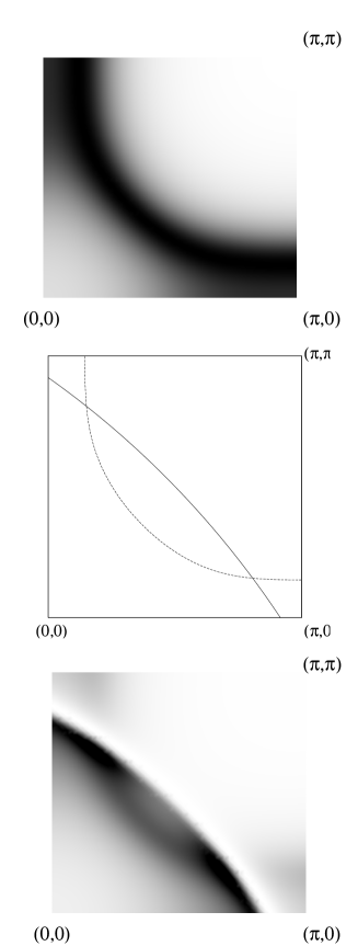
FIG. 16.: (a) Gray scale plot of the spectral intensity immediately below $E_{F}$, computed from (48) with $A(\omega)=1$.
(b) Fermi surface (dashed line) and constant energy contour of the surface state (full line).
(c) Spectral intensity in the presence of the surface state, i.e. (48) with the true $A(\omega)$.

The latter is shown in Figure 16b. In Figure 16c, on the other hand, we have included the Fano curve $A(\omega)$ for the surface state with $\mathchoice{{\hbox{\boldmath$\displaystyle G$}}}{{\hbox{\boldmath$\textstyle G$}}}{{\hbox{\boldmath$\scriptstyle G$}}}{{\hbox{\boldmath$\scriptscriptstyle G$}}}_{\|}=(-2\pi,-2\pi)$ (assuming a free 2D-electron dispersion with lattice constant $2.82Angstrom$) and a kinetic energy of $T=33eV$. The corresponding constant energy-contour $\frac{4\pi^{2}\hbar^{2}}{2ma^{2}}(\mathchoice{{\hbox{\boldmath$\displaystyle k$}}}{{\hbox{\boldmath$\textstyle k$}}}{{\hbox{\boldmath$\scriptstyle k$}}}{{\hbox{\boldmath$\scriptscriptstyle k$}}}+\mathchoice{{\hbox{\boldmath$\displaystyle G$}}}{{\hbox{\boldmath$\textstyle G$}}}{{\hbox{\boldmath$\scriptstyle G$}}}{{\hbox{\boldmath$\scriptscriptstyle G$}}})^{2}=33eV$ is also shown in Figure 17. One can see quite clearly then, that the contour attenuates the true Fermi surface on its ‘backside’ and strongly enhances the intensity at its ‘frontside’ thus creating the rather perfect impression of a Fermi surface arc which intersects the $(1,0)$ direction at approximately $(0.8\pi,0)$. On the other hand in our model the true Fermi surface is the one seen in Figure 16a. The combination of Fano resonance and flat band portion near $(\pi,0)$ thus produces an ‘apparent Fermi surface’ which is entirely artificial.
To compare with experimental data in more detail, we recall that upon neglecting the dispersion of the valence band state as compared to that of the surface resonance, the momenta in the $\mathchoice{{\hbox{\boldmath$\displaystyle k$}}}{{\hbox{\boldmath$\textstyle k$}}}{{\hbox{\boldmath$\scriptstyle k$}}}{{\hbox{\boldmath$\scriptscriptstyle k$}}}_{\|}$-plane where intersections as the one in Figure 14 occur have to obey the equation

$\displaystyle T=\frac{\hbar^{2}(\mathchoice{{\hbox{\boldmath$\displaystyle k$}}}{{\hbox{\boldmath$\textstyle k$}}}{{\hbox{\boldmath$\scriptstyle k$}}}{{\hbox{\boldmath$\scriptscriptstyle k$}}}_{\|}+\mathchoice{{\hbox{\boldmath$\displaystyle G$}}}{{\hbox{\boldmath$\textstyle G$}}}{{\hbox{\boldmath$\scriptstyle G$}}}{{\hbox{\boldmath$\scriptscriptstyle G$}}})^{2}}{2m},$

where $T$ denotes the kinetic energy of the ejected electron. In other words: the resonant enhancement of the ARPES intensity occurs along a constant energy contour of the surface resonance dispersion. If we stick to our free-electron approximation, these are simply circles in the $\mathchoice{{\hbox{\boldmath$\displaystyle k$}}}{{\hbox{\boldmath$\textstyle k$}}}{{\hbox{\boldmath$\scriptstyle k$}}}{{\hbox{\boldmath$\scriptscriptstyle k$}}}_{\|}$-plane centered on $-\mathchoice{{\hbox{\boldmath$\displaystyle G$}}}{{\hbox{\boldmath$\textstyle G$}}}{{\hbox{\boldmath$\scriptstyle G$}}}{{\hbox{\boldmath$\scriptscriptstyle G$}}}$. Figure 17 then shows these contours for two different photon energies, namely $22\;eV$ and $34\;ev$. Thereby we have again assumed that $T=h\nu-8\;eV$. Also shown is the standard ‘Fermi surface’, determined at $22\;eV$. It is then obvious that the ‘$22\;eV$-Fermi surface’ always is close to some portion of a surface resonance contour. This would imply that for this photon energy most potions of the Fermi surface could be enhanced - it might also be taken to suggest, however, that some Fermi surface portions near $(\pi,0)$ are actually artificial. It is hard to give a more detailed discussion, because even slight deviations from the free electron dispersion for the surface resonance will have a major impact on the energy contours. For $34\;eV$, on the other hand, the Fermi surface obviously is ‘cut off’ near $(\pi,0)$ by the contour for ${\bf G}=2\pi\;(-2,0)$. The Fermi surface seen at $34\;eV$ then might be obtained by following the true Fermi contour (dashed line) until the intersection with the $(-2,0)$-contour, and then following the latter (where the ARPES intensity is high due to the resonance effect and the fact there are states immediately below $\mu$ due to the flat band around $(\pi,0)$). In this way one would obtain a ‘Fermi contour’ which is quite similar to the one actually observed at $34\;eV$. For even higher photon energy there are too many $\textstyle G$’s which contribute their own circles, so that one cannot give a meaningful discussion.

FIG. 17.: (a) The full lines give the constant energy contours for a free electron-like surface resonance state for kinetic energy $22\;eV-8\;eV$ (a) and $34\;eV-8\;eV$ (b). The dashed line is the ‘Fermi surface’ seen in Bi2212.

The question which of the different Fermi surface portions observed in Bi2212 are artificial and which are real clearly needs a detailed experimental study. A very simple way would be to vary the photon energy in small steps of (e.g.) $1eV$, in which case one should observe a continuous drift of the ‘Fermi surface’ for those parts which are artificial. Unfortunately the present understanding of surface resonances in cuprate materials is much too rudimentary to make any theoretical prediction. Not even knowing any details of their dispersion, we have to content ourselves with the very much oversimplified model calculations outlined above to show what might happen. Even these simple model calculations do show rather clearly, however, that simply plotting intensity maps near $E_{F}$ or identifying ‘Fermi surface crossings’ near $(\pi,0)$ by drops of spectral weight is not really an adequate means to clarify this issue.

VII Conclusion

In summary, we have presented a discussion of ARPES intensities from the CuO₂ plane. Thereby we could actually address only a few (but hopefully the most important) aspects of the problem.
To begin with, the geometry of the orbitals, which form the first ionization states of the CuO₂ plane, leads to a pronounced anisotropy of the photoelectron current. This makes itself felt in a strong dependence of the intensity on the polarization of the incoming light. This may be exploited to enhance the intensity seen in an ARPES experiment by choosing appropriate photon polarization or going to a higher Brillouin zone. We have presented a simple model to guess ‘optimized’ values of the polarization and the Brillouin zone to obtain maximum intensity for a given ${\bf k}$-point.
Moreover there is a strong preference for a Zhang-Rice singlet to emit photoelectrons at small angles relative to the plane. This in turn may lead to a injection of the photoelectrons into states located at the surface of the sample, so-called surface resonances. Such surface resonances are well-established in at least one cuprate-related material, namely Sr₂CuCl₂O₂. We have proposed to explain the pronounced photon-energy dependence of the ARPES intensities in this material by these surface resonances. Next, we have presented a simple model calculation which shows how such surface resonances may lead to apparent Fermi surfaces in the flat-band region around $(\pi,0)$. This may be one explanation for the apparently different Fermi surface topology seen in Bi2212 at $22\;eV$ and at $34\;eV$, possibly also in an interplay with bilayer-splitting[21, 22]. In any case the existence or non-existence of surface-resonances should be clarified experimentally, since the identification of any major Fermi surface portion near $(\pi,0)$ as being ‘artificial’ amy have major implications for our understanding of cuprate materials.
Acknowledgment: Instructive discussions with V. Borisenko, J. Fink, M. Golden and A. Fleszar are most gratefully acknowledged. This work is supported by the projects DFG HA1537/20-2, KONWIHR OOPCV and BMBF 05SB8WWA1. Support by computational facilities of HLRS Stuttgart and LRZ Munich is acknowledged.

VIII Appendix I:Calculation of Radial Matrix Elements

The actual calculation of the radial matrix elements $R_{l,l^{\prime}}$ prove to be one of the most crucial points when making contact with experimental results. Functional forms of effective potentials for the CuO₂ compound are not known. A simple approach with a hydrogen-like potential seems doubtful, if one attempts cover at least a certain amount of physical reality of the photoemission process. A good starting point for an at least qualitative derivation of the matrix elements are the radial wave functions that can be obtained from density functional calculations, which include information about the electron-electron exchange correlation and the screening of the nuclear charge. The radial matrix elements used in this paper are calculated in the local-density approximation, where one solves the effective one electron Schrödinger equation

$$\left(\frac{1}{2}\nabla^{2}+v^{\alpha,\sigma}_{\mbox{eff}}\left({\bf r}\right)\right)\psi_{\alpha,\sigma}=\epsilon^{LDA}_{\alpha,\sigma}\psi_{\alpha,\sigma}\left({\bf r}\right).$$ (53)

The potential $v^{\alpha,\sigma}_{\mbox{eff}}\left({\bf r}\right)$ is a functional of the electron density, given by

$\displaystyle v^{\alpha,\sigma}_{\mbox{eff}}\left({\bf r}\right)=\left(v\left({\bf r}\right)+u\left([n];{\bf r}\right)+v^{\sigma}_{\mbox{xc}}\left(\left[n_{\uparrow},n_{\downarrow}\right];{\bf r}\right)\right).$

$v({\bf r})$ is the full nuclear potential and $u\left([n];{\bf r}\right)$ the direct Coulomb-potential $\int d{\bf r}^{\prime}n\left({\bf r}^{\prime}\right)/\left|{\bf r}-{\bf r}^{\prime}\right|$. The exchange-correlation functional $v^{\sigma}_{\mbox{xc}}\left(\left[n_{\uparrow},n_{\downarrow}\right];{\bf r}\right)$ is a parameterized after Ref. [27]. Equation (53) is solved selfconsistently to convergence of the total energy, resulting in a set of energy eigenvalues $\epsilon_{n}$ and radial wave functions $R_{n,l}(r)$, which we used to calculate

$\displaystyle R_{ll^{\prime}}(E)=\int drr^{3}R_{E,l}(r)R_{n,l}(r).$

Since we assume emitted electrons to be approximated by plane waves at the detection point, additional information on the outgoing wave function is needed in form of the phase shift compared to the asymptotic behaviour of

$\displaystyle R^{asym}_{El}(r)\approx 2\frac{\sin\left(kr-\frac{l\pi}{2}+\delta_{l}\right)}{r},\qquad r\rightarrow\infty,$

defining the interference of wave functions emitted by Op_x,y and Cud${}_{x^{2}-y^{2}}$ orbitals. The phase shift can easily be found by comparing the logarithmic derivatives

$\displaystyle\left(\frac{\partial}{\partial r}R\left(r\right)\right)/R\left(r\right)=\left(\frac{\partial}{\partial r}R^{asym}_{El}\left(r\right)\right)/R^{asym}_{El}\left(r\right)$

at a sufficiently large radius where

$\displaystyle\frac{\partial}{\partial r}v^{\alpha,\sigma}_{\mbox{eff}}\left({\bf r}\right)\approx 0.$

FIG. 18.: Radial integrals R${}_{l,l^{\prime}}$ (top) and Scattering phases $\delta_{l,l^{\prime}}$ (bottom) as calculated from density functional theory.

IX Appendix II

Here we present in more detail the calculation of the vectors $\textstyle v$ of interest to us. For the CEF initial states of interest to us, such as $p_{x}$, $p_{y}$ and $d_{x^{2}-y^{2}}$, the coefficients $c_{\alpha m^{\prime}}$ take the form

$\displaystyle c_{\alpha m^{\prime}}=\frac{\zeta}{\sqrt{2}}\;(\delta_{m^{\prime},\nu}\pm\delta_{m^{\prime},-\nu}),$

(see Table I) whence we find that

$$\sum_{m}\;d_{lm}\;Y_{lm}(\mathchoice{{\hbox{\boldmath$\displaystyle k$}}}{{\hbox{\boldmath$\textstyle k$}}}{{\hbox{\boldmath$\scriptstyle k$}}}{{\hbox{\boldmath$\scriptscriptstyle k$}}}^{0}) = \sqrt{\frac{4\pi}{3}}\sum_{\mu=-1}^{1}\;Y_{1,\mu}^{*}(\mathchoice{{\hbox{\boldmath$\displaystyle\epsilon$}}}{{\hbox{\boldmath$\textstyle\epsilon$}}}{{\hbox{\boldmath$\scriptstyle\epsilon$}}}{{\hbox{\boldmath$\scriptscriptstyle\epsilon$}}})\;A_{l,\mu}(\mathchoice{{\hbox{\boldmath$\displaystyle k$}}}{{\hbox{\boldmath$\textstyle k$}}}{{\hbox{\boldmath$\scriptstyle k$}}}{{\hbox{\boldmath$\scriptscriptstyle k$}}}^{0})$$ (54)

$$A_{l,\mu}(\mathchoice{{\hbox{\boldmath$\displaystyle k$}}}{{\hbox{\boldmath$\textstyle k$}}}{{\hbox{\boldmath$\scriptstyle k$}}}{{\hbox{\boldmath$\scriptscriptstyle k$}}}^{0}) = \frac{\zeta}{\sqrt{2}}\;\left(Y_{l,\mu+\nu}(\mathchoice{{\hbox{\boldmath$\displaystyle k$}}}{{\hbox{\boldmath$\textstyle k$}}}{{\hbox{\boldmath$\scriptstyle k$}}}{{\hbox{\boldmath$\scriptscriptstyle k$}}}^{0})\;c^{1}(l,\mu+\nu;l^{\prime},\nu)\pm Y_{l,\mu-\nu}(\mathchoice{{\hbox{\boldmath$\displaystyle k$}}}{{\hbox{\boldmath$\textstyle k$}}}{{\hbox{\boldmath$\scriptstyle k$}}}{{\hbox{\boldmath$\scriptscriptstyle k$}}}^{0})\;c^{1}(l,\mu-\nu;l^{\prime},-\nu)\right)$$ (55)

We now rewrite the scalar product

$\displaystyle\sqrt{\frac{4\pi}{3}}\sum_{\mu=-1}^{1}\;Y_{1,\mu}^{*}(\mathchoice{{\hbox{\boldmath$\displaystyle\epsilon$}}}{{\hbox{\boldmath$\textstyle\epsilon$}}}{{\hbox{\boldmath$\scriptstyle\epsilon$}}}{{\hbox{\boldmath$\scriptscriptstyle\epsilon$}}})\;A_{\mu}^{l}=\mathchoice{{\hbox{\boldmath$\displaystyle\epsilon$}}}{{\hbox{\boldmath$\textstyle\epsilon$}}}{{\hbox{\boldmath$\scriptstyle\epsilon$}}}{{\hbox{\boldmath$\scriptscriptstyle\epsilon$}}}\cdot\mathchoice{{\hbox{\boldmath$\displaystyle A$}}}{{\hbox{\boldmath$\textstyle A$}}}{{\hbox{\boldmath$\scriptstyle A$}}}{{\hbox{\boldmath$\scriptscriptstyle A$}}}_{l}$

and by use of the property $c^{1}(l,-m;l^{\prime},-m^{\prime})=c^{1}(l,m;l^{\prime},m^{\prime})$ we obtain the components of $\mathchoice{{\hbox{\boldmath$\displaystyle A$}}}{{\hbox{\boldmath$\textstyle A$}}}{{\hbox{\boldmath$\scriptstyle A$}}}{{\hbox{\boldmath$\scriptscriptstyle A$}}}^{l}$:

$$A_{l,x} = \frac{1}{\sqrt{2}}\;[\;c^{1}(l,\nu-1;l^{\prime},\nu)\;\frac{\zeta}{\sqrt{2}}\;(Y_{l,\nu-1}\mp Y_{l,-(\nu-1)})-c^{1}(l,\nu+1;l^{\prime},\nu)\;\frac{\zeta}{\sqrt{2}}\;(Y_{l,\nu+1}\mp Y_{l,-(\nu+1)})\;],$$ (56)

$$A_{l,y} = \frac{i}{\sqrt{2}}\;[\;c^{1}(l,\nu-1;l^{\prime},\nu)\;\frac{\zeta}{\sqrt{2}}\;(Y_{l,\nu-1}\pm Y_{l,-(\nu-1)})+c^{1}(l,\nu+1;l^{\prime},\nu)\;\frac{\zeta}{\sqrt{2}}\;(Y_{l,\nu+1}\pm Y_{l,-(\nu+1)})\;],$$ (57)

$$A_{l,z} = c^{1}(l\nu;l^{\prime}\nu)\;\frac{\zeta}{\sqrt{2}}(Y_{l,\nu}\pm Y_{l,-\nu}).$$ (58)

Defining $\tilde{R}_{l,l^{\prime}}(E)=\;e^{i\delta_{l}}R_{l,l^{\prime}}(E)$ we now readily arrive at the following expressions for photocurrent:

$${\bf j} = \frac{4N\hbar{\bf k}}{m}\;|\mathchoice{{\hbox{\boldmath$\displaystyle v$}}}{{\hbox{\boldmath$\textstyle v$}}}{{\hbox{\boldmath$\scriptstyle v$}}}{{\hbox{\boldmath$\scriptscriptstyle v$}}}\cdot\mathchoice{{\hbox{\boldmath$\displaystyle\epsilon$}}}{{\hbox{\boldmath$\textstyle\epsilon$}}}{{\hbox{\boldmath$\scriptstyle\epsilon$}}}{{\hbox{\boldmath$\scriptscriptstyle\epsilon$}}}|^{2},$$ (59)

$$v = \sum_{l=l^{\prime}\pm 1}(-i)^{l+1}\;\tilde{R}_{l,l^{\prime}}(E)\;\mathchoice{{\hbox{\boldmath$\displaystyle A$}}}{{\hbox{\boldmath$\textstyle A$}}}{{\hbox{\boldmath$\scriptstyle A$}}}{{\hbox{\boldmath$\scriptscriptstyle A$}}}_{l}.$$ (60)

Here the vector $\textstyle v$ depends on the type of initial orbital. Straightforward algebra then yields the following expressions for the vectors $\textstyle v$:

$$\mathchoice{{\hbox{\boldmath$\displaystyle v$}}}{{\hbox{\boldmath$\textstyle v$}}}{{\hbox{\boldmath$\scriptstyle v$}}}{{\hbox{\boldmath$\scriptscriptstyle v$}}}(p_{x}) = \sqrt{\frac{1}{15}}\tilde{R}_{21}\left(\begin{array}[]{c}\sqrt{\frac{5}{4\pi}}\frac{\tilde{R}_{01}}{\tilde{R}_{21}}+d_{3z^{2}-r^{2}}(\mathchoice{{\hbox{\boldmath$\displaystyle k$}}}{{\hbox{\boldmath$\textstyle k$}}}{{\hbox{\boldmath$\scriptstyle k$}}}{{\hbox{\boldmath$\scriptscriptstyle k$}}}^{0})-\sqrt{3}d_{x^{2}-y^{2}}(\mathchoice{{\hbox{\boldmath$\displaystyle k$}}}{{\hbox{\boldmath$\textstyle k$}}}{{\hbox{\boldmath$\scriptstyle k$}}}{{\hbox{\boldmath$\scriptscriptstyle k$}}}^{0})\\ -\sqrt{3}d_{xy}(\mathchoice{{\hbox{\boldmath$\displaystyle k$}}}{{\hbox{\boldmath$\textstyle k$}}}{{\hbox{\boldmath$\scriptstyle k$}}}{{\hbox{\boldmath$\scriptscriptstyle k$}}}^{0})\\ -\sqrt{3}d_{xz}(\mathchoice{{\hbox{\boldmath$\displaystyle k$}}}{{\hbox{\boldmath$\textstyle k$}}}{{\hbox{\boldmath$\scriptstyle k$}}}{{\hbox{\boldmath$\scriptscriptstyle k$}}}^{0})\end{array}\right)$$ (64)

$$\mathchoice{{\hbox{\boldmath$\displaystyle v$}}}{{\hbox{\boldmath$\textstyle v$}}}{{\hbox{\boldmath$\scriptstyle v$}}}{{\hbox{\boldmath$\scriptscriptstyle v$}}}(p_{y}) = \sqrt{\frac{1}{15}}\tilde{R}_{21}\left(\begin{array}[]{c}-\sqrt{3}d_{xy}(\mathchoice{{\hbox{\boldmath$\displaystyle k$}}}{{\hbox{\boldmath$\textstyle k$}}}{{\hbox{\boldmath$\scriptstyle k$}}}{{\hbox{\boldmath$\scriptscriptstyle k$}}}^{0})\\ \sqrt{\frac{5}{4\pi}}\frac{\tilde{R}_{01}}{\tilde{R}_{21}}+d_{3z^{2}-r^{2}}(\mathchoice{{\hbox{\boldmath$\displaystyle k$}}}{{\hbox{\boldmath$\textstyle k$}}}{{\hbox{\boldmath$\scriptstyle k$}}}{{\hbox{\boldmath$\scriptscriptstyle k$}}}^{0})+\sqrt{3}d_{x^{2}-y^{2}}(\mathchoice{{\hbox{\boldmath$\displaystyle k$}}}{{\hbox{\boldmath$\textstyle k$}}}{{\hbox{\boldmath$\scriptstyle k$}}}{{\hbox{\boldmath$\scriptscriptstyle k$}}}^{0})\\ -\sqrt{3}d_{yz}(\mathchoice{{\hbox{\boldmath$\displaystyle k$}}}{{\hbox{\boldmath$\textstyle k$}}}{{\hbox{\boldmath$\scriptstyle k$}}}{{\hbox{\boldmath$\scriptscriptstyle k$}}}^{0})\end{array}\right)$$ (68)

$$\mathchoice{{\hbox{\boldmath$\displaystyle v$}}}{{\hbox{\boldmath$\textstyle v$}}}{{\hbox{\boldmath$\scriptstyle v$}}}{{\hbox{\boldmath$\scriptscriptstyle v$}}}(p_{z}) = \sqrt{\frac{1}{15}}\tilde{R}_{21}\left(\begin{array}[]{c}-\sqrt{3}d_{xz}(\mathchoice{{\hbox{\boldmath$\displaystyle k$}}}{{\hbox{\boldmath$\textstyle k$}}}{{\hbox{\boldmath$\scriptstyle k$}}}{{\hbox{\boldmath$\scriptscriptstyle k$}}}^{0})\\ -\sqrt{3}d_{yz}(\mathchoice{{\hbox{\boldmath$\displaystyle k$}}}{{\hbox{\boldmath$\textstyle k$}}}{{\hbox{\boldmath$\scriptstyle k$}}}{{\hbox{\boldmath$\scriptscriptstyle k$}}}^{0})\\ \sqrt{\frac{5}{4\pi}}\frac{\tilde{R}_{01}}{\tilde{R}_{21}}+\sqrt{4}d_{3z^{2}-r^{2}}(\mathchoice{{\hbox{\boldmath$\displaystyle k$}}}{{\hbox{\boldmath$\textstyle k$}}}{{\hbox{\boldmath$\scriptstyle k$}}}{{\hbox{\boldmath$\scriptscriptstyle k$}}}^{0})\end{array}\right)$$ (72)

With the exception of the numerical prefactors, most of the above formulas could have been guessed from general principles: there are only transitions into $s$-like and $d$-like partial waves (i.e. the dipole selection rule $\Delta L=\pm 1$!) and acting e.g. with an electric field in $x$ direction onto a $p_{x}$ -orbital produces only $s$-like, $d_{x^{2}-y^{2}}$-like and $d_{3z^{2}-r^{2}}$-like partial waves (which have even parity under reflection by the $z-y$-plane), whereas acting with a field in $y$ direction on $p_{x}$ can only produce the $d_{xy}$ partial wave. We therefore believe that much of the formula remains true even if more realistic wave functions for the final states are chosen.
Similarly, we find for the matrix element of the $d$-like orbitals:

$${\bf v}\left(d_{3z^{2}-r^{2}}\right) = i\left(\matrix{\frac{1}{\sqrt{30}}\tilde{R}_{12}p_{x}+\sqrt{\frac{3}{35}}\tilde{R}_{32}f_{5x(z^{2}-r^{2})}\cr\frac{1}{\sqrt{30}}\tilde{R}_{12}p_{y}+\sqrt{\frac{3}{35}}\tilde{R}_{32}f_{5y(z^{2}-r^{2})}\cr-\frac{2}{\sqrt{15}}\tilde{R}_{12}p_{z}+\frac{3}{\sqrt{35}}\tilde{R}_{32}f_{z(5z^{2}-3r^{2})}}\right)$$ (73)

$${\bf v}\left(d_{yz}\right) = i\left(\matrix{\frac{1}{\sqrt{7}}\tilde{R}_{32}f_{xyz}\cr-\frac{1}{\sqrt{5}}\tilde{R}_{12}p_{z}-\sqrt{\frac{3}{35}}\tilde{R}_{32}f_{5z^{3}-3z}-\frac{1}{\sqrt{7}}\tilde{R}_{32}f_{z(x^{2}-y^{2})}\cr-\frac{1}{\sqrt{5}}\tilde{R}_{12}p_{y}+\sqrt{\frac{8}{35}}\tilde{R}_{32}f_{y(5z^{2}-1)}}\right)$$ (74)

$${\bf v}\left(d_{xz}\right) = i\left(\matrix{-\frac{1}{\sqrt{5}}\tilde{R}_{12}p_{z}-\sqrt{\frac{3}{35}}\tilde{R}_{32}f_{5z^{2}-3z}+\frac{1}{\sqrt{7}}\tilde{R}_{32}f_{z(x^{2}-y^{2})}\cr\frac{1}{\sqrt{7}}\tilde{R}_{32}f_{xyz}\cr-\frac{1}{\sqrt{5}}\tilde{R}_{12}p_{x}+\sqrt{\frac{8}{35}}\tilde{R}_{32}f_{x(5z^{2}-1)}}\right)$$ (75)

$${\bf v}\left(d_{x^{2}-y^{2}}\right) = i\left(\matrix{-\frac{1}{\sqrt{5}}\tilde{R}_{12}p_{x}-\frac{1}{\sqrt{70}}\tilde{R}_{32}f_{x(5z^{2}-1)}+\sqrt{\frac{3}{14}}\tilde{R}_{32}f_{x^{3}-3xy^{2}}\cr\frac{1}{\sqrt{5}}\tilde{R}_{12}p_{y}+\frac{1}{\sqrt{70}}\tilde{R}_{32}f_{y(5z^{2}-1)}+\sqrt{\frac{3}{14}}\tilde{R}_{32}f_{3yx^{2}-y^{3}}\cr\frac{1}{\sqrt{7}}\tilde{R}_{32}f_{z(x^{2}-y^{2})}}\right)$$ (76)

$${\bf v}\left(d_{xy}\right) = i\left(\matrix{-\frac{1}{\sqrt{5}}\tilde{R}_{12}p_{y}-\frac{1}{\sqrt{70}}\tilde{R}_{32}f_{y(5z^{2}-1)}+\sqrt{\frac{3}{14}}\tilde{R}_{32}f_{yx^{2}-y^{3}}\cr-\frac{1}{\sqrt{5}}\tilde{R}_{12}p_{x}-\frac{1}{\sqrt{70}}\tilde{R}_{32}f_{x(5z^{2}-1)}-\sqrt{\frac{3}{14}}\tilde{R}_{32}f_{x^{3}-xy^{2}}\cr\frac{1}{\sqrt{7}}\tilde{R}_{32}f_{xyz}}\right)$$ (77)

With the exception of the numerical prefactors, most of the above formulas could have been guessed from general principles: there are only transitions into $s$-like and $d$-like partial waves (i.e. the dipole selection rule $\Delta L=\pm 1$!) and acting e.g. with an electric field in $x$ direction onto a $p_{x}$ -orbital produces only $s$-like, $d_{x^{2}-y^{2}}$-like and $d_{3z^{2}-r^{2}}$-like partial waves (which have even parity under reflection by the $z-y$-plane), whereas acting with a field in $y$ direction on $p_{x}$ can only produce the $d_{xy}$ partial wave. We therefore believe that much of the formula remains true even if more realistic wave functions for the final states are chosen.

Gx/$2\pi$	Gy/$2\pi$	$\phi^{(opt)}_{E}$	$I/I_{0}$	$\phi^{(opt)}_{E}$	$\theta^{(opt)}_{E}$	$I/I_{0}$	$h\nu$
-1	-1	2.356	1.908	2.356	1.571	1.908	22eV
-1	0	1.275	0.958	1.275	1.005	1.345	22eV
0	-1	0.295	0.958	0.295	1.005	1.345	22eV
0	0	2.356	1.000	2.356	1.571	1.000	22eV
-1	-1	2.356	2.011	2.356	1.571	2.011	34eV
-1	0	0.974	1.053	0.974	1.040	1.417	34eV
-1	1	1.426	2.255	1.426	0.964	3.342	34eV
0	-1	0.597	1.053	0.597	1.040	1.417	34eV
0	0	2.356	1.000	2.356	1.571	1.000	34eV
0	1	2.218	0.913	2.190	0.754	1.922	34eV
1	-1	0.145	2.255	0.145	0.964	3.342	34eV
1	0	2.494	0.913	2.523	2.388	1.922	34eV

TABLE I.: Intensities of the ZRS relative to $k=(\frac{\pi}{2},\frac{\pi}{2})$ in higher Brillouin zones ${\bf k}+{\bf G}$ for 22 and 34eV photon energy.

Gx/$2\pi$	Gy/$2\pi$	$\phi^{(opt)}_{E}$	$I/I_{0}$	$\phi^{(opt)}_{E}$	$\theta^{(opt)}_{E}$	$I/I_{0}$	$h\nu$
-1	-1	2.422	4.313	2.419	1.806	4.563	22eV
-1	0	0.000	1.000	0.000	0.556	3.436	22eV
-1	1	0.719	4.313	0.723	1.335	4.563	22eV
0	-1	0.719	4.313	0.723	1.806	4.563	22eV
0	0	0.000	1.000	0.000	2.586	3.436	22eV
0	1	2.422	4.313	2.419	1.335	4.563	22eV
-2	0	0.000	1.645	0.000	2.318	3.058	34eV
-1	-1	2.472	2.588	2.466	1.963	3.019	34eV
-1	0	0.000	1.000	0.000	0.751	2.133	34eV
-1	1	0.669	2.588	0.675	1.178	3.019	34eV
0	-1	0.669	2.588	0.675	1.963	3.019	34eV
0	0	0.000	1.000	0.000	2.391	2.133	34eV
0	1	2.472	2.588	2.466	1.178	3.019	34eV
1	0	0.000	1.645	0.000	0.823	3.058	34eV

TABLE II.: Intensities of the ZRS relative to $k=(\pi,0)$ in higher Brillouin zones ${\bf k}+{\bf G}$ for 22 and 34eV photon energy.

REFERENCES

[1] Z.-X. Shen and D. S. Dessau, Phys. Rep. 253 1 (1995).
[2] B. O. Wells, Z.-X. Shen, A. Matsuura, D. King, M. Kastner, M. Greven, and
R. J. Birgenau, Phys. Rev. Lett. 74, 964 (1995).
[3] F. Ronning, C. Kim, D.L. Feng, D.S. Marshall, A.G. Loeser, L.L. Miller, J.N.
Eckstein, I. Bozovic, and Z.-X. Shen, Science, 282, 2067 (1998).
[4]
S. V. Borisenko, M. S. Golden, S. Legner, T. Pichler, C.Duerr, M.Knupfer,
J. Fink, G.Yang, S. Abell, and H.Berger,
Phys. Rev. Lett. 83, 3717 (1999).
[5]
H.M. Fretwell, A. Kaminski, J. Mesot, J.C. Campuzano, M.R. Norman,
M. Randeria, T. Sato, R. Gatt, T. Takahashi, and K. Kadowaki,
Phys. Rev. Lett. 84, 4449 (2000)
[6]
J. Mesot et. al., Phys. Rev. B 63, 224516-1 (2001)
[7]
Y. D. Chuang, A. D. Gromko, D. S. Dessau, Y. Aiura, Y. Yamaguchi, K. Oka,
A. J. Arko, J. Joyce, H. Eisaki, S.I. Uchida, K. Nakamura, and Yoichi Ando,
Phys. Rev. Lett. 83, 3717 (1999).
[8]
D.L. Feng, W.J. Zheng, K.M. Shen, D.H. Lu, F. Ronning, J.-I. Shimoyama,
K. Kishio, G. Gu, D. Van der Marel, and Z.-X. Shen,
cond-mat/9908056.
[9]
A.D. Gromko, Y.-D. Chuang, D.S. Dessau, K. Nakamura, and Yoichi Ando,
cond-mat/0003017.
[10]
P. V. Bogdanov, A. Lanzara, X. J. Zhou, S. A. Kellar, D.L. Feng, E. D. Lu,
J.-I. Shimoyama, K. Kishio, Z. Hussain, and Z.-X. Shen, cond-mat/0005394.
[11]et. al Phys. Rev. B 63, 14505 (2000)
[12] F. C. Zhang and T. M. Rice, PRB 37 3759 (1988).
[13] T. Matsushita, S. Imada, H. Daimon, T. Okuda, K. Yamaguchi,
H. Miyagi, and S. Suga, Phys. Rev. B 56 7687 (1997).
[14] A. S. Moskvin, E. N. Kondrashov, V. I. Cherepanov
cond-mat 0007470 (2001).
[15]
J. C. Slater, Quantum Theory of Atomic Structure
McGraw-Hill Book Company, New York Toronto London (1960);
see in particular Appendix 20 of Volume II.
[16] O. K. Andersen, A. I. Liechtenstein, O. Jepsen, and F. Paulsen,
J. Phys. Chem. Solids 56, 1573 (1995).
[17] A. Bansil and M. Lindroos
Phys. Rev. Lett. 83, 5154 (1999)
[18]D. Sénéchal, D. Perez and M. Pioro-Ladrière,
Phys. Rev. Lett. 84, 522 (2000).
[19] B. K. Theo, ‘EXFAS: Basic Principles and Data Analysis’, Springer, Berlin (1986).
[20] R. Manzke et. al
Phys. Rev. B 63, 100504 (2001).
[21] D. L. Feng, N. P. Armitage, D. H. Lu, A. Damascelli,
J. P. Hu, P. Bogdanov, A. Lanzara, F. Ronning, K. M. Shen, H. Eisaki,
C. Kim, Z. X. Shen, Phys. Rev. Lett. 86, 5550 (2001).
[22] Y.-D. Chuang, A. D. Gromko, A. V. Fedorov, Y. Aiura, K. Oka,
Yoichi Ando, D. S. Dessau, cond-mat/0107002 (2001).
[23] A. Gerlach, R. Matzdorf and A. Goldmann,
Phys. Rev. B 58, 10969 (1998).
[24] E. G. McRae, Rev. Mod. Phys. 51, 541 (1979).
[25] J. J. M. Pothuizen,
‘Electrons in and close to Correlated Systems’, Thesis,
Rijksuniversiteit Groningen (1998). The parts about the surface resonance are
unpublished, but can be downloaded from
http://www.ub.rug.nl/eldoc/dis/science/j.j.m.pothuizen/
[26]
R. J . Radtke and M. R. Norman, cond-mat/9404081
[27]
J. P. Perdew and A. Zunger, Phys. Rev. B 23, 5048 (1981).