Asset-asset interactions and clustering
in financial markets

Abstract

The collective phenomena of a liquid market is characterized in terms of a particle system scenario. This physical analogy enables us to disentangle intrinsic features from purely stochastic ones. The latter are the result of environmental changes due to a ‘heat bath’ acting on the many-asset system, quantitatively described in terms of a time dependent effective temperature. The remaining intrinsic properties can be widely investigated by applying standard methods of classical many body systems. As an example, we consider a large set of stocks traded at the NYSE and determine the corresponding asset–asset ‘interaction’ potential. In order to investigate in more detail the cluster structure suggested by the short distance behavior of the interaction potential, we perform a connectivity analysis of the spatial distribution of the particle system. In this way, we are able to draw conclusions on the intrinsic cluster persistency independently of the specific market conditions.

, , and

The stochastic character of financial market time series is one of their distinct aspects. Despite this random behavior, evidence has been found recently that a certain degree of correlation is still present on extremely short time scales [1]. The possibility to anticipate the future evolution of a single asset from the knowledge of its past values is however minimized by the presence of traders active on short time scales, usually with delays smaller than few seconds.

Time dependence is just one possible domain for investigating correlation patterns inside financial signals (see [2] and [3]), if contrasted with ‘spatial’ one, in which the features of interest are commonly referred to as multivariate correlations. In such a spatial domain, a financial market is seen as a complex system of interacting constituents [4], where the study of correlations among different assets is of peculiar importance, as in the modern theory of risk management. On a more fundamental level, an interesting issue is to understand how price changes can be separated, with a sufficient degree of confidence, into single asset, and collective, behavior.

In this paper, we are concerned with a method recently proposed to investigate asset correlations in a stock market by means of a particle system scenario. This can be achieved by introducing a formal map between logarithmic returns and distances among particles in a classical liquid [5]. The power of this analogy consists in the possibility of separating collective motion from the single asset dynamics, by determining the mutual interactions among the different assets. In this way, we can study the ‘thermodynamics’ of the system, interpreting its temperature as a measure of spatial volatility, which can be regarded as the counterpart of the more familiar (temporal) volatility. The 2, asset interaction potential is then calculated on the isothermal (isovolatile) market. In the following, the concept of time dependent asset, asset distance and the moving frame of reference model of Ref. [5] are reviewed. The asset, asset effective pair potential is obtained from a daily stock data taken from the New York Stock Exchange (NYSE). The phenomenon of asset clustering is also discussed, followed by the concluding remarks.

We consider a collection of $N$ assets from a given stock market. We wish to define a ‘metric’ within such a subspace of assets, so that a ‘distance’ between any two assets can be determined using only information of asset values at different time horizons. The value of asset $i$ at time $t$, $\Omega_{i}(t)$, can be expressed in units of the value of asset $j$, $\Omega_{j}(t)$, by means of the conversion factor $P_{ij}(t)$, as $\Omega_{i}(t)=P_{ij}(t)\Omega_{j}(t)$. By writing $\Omega_{i}$ as a function of $\Omega_{k}$, and the latter as a function of $\Omega_{j}$, the no, arbitrage equation for a liquid market is obtained $P_{ij}=P_{ik}P_{kj}$ [5]. The latter implicitly defines all the cross-ratios $P_{ij}$ for any index $i,j$.

According to [5], the quantity $d^{\alpha}_{ij}(t)=(1/{\tau_{\alpha}})\log[P_{ij}(t)/P_{ij}(t-\tau_{\alpha})]$ can be identified as the $\alpha$–component of a position vector between assets $i$ and $j$, ${\mathbf{d}}_{ij}$. It is natural to take $\tau_{\alpha}$ from a collection of $H$ time horizons, where $\alpha\leq H$. In the $H$–dimensional space, ${\mathbf{d}}_{ij}$ obeys the vector relations: (a) ${\mathbf{d}}_{ii}\equiv{\mathbf{0}}$, (b) ${\mathbf{d}}_{ij}=-{\mathbf{d}}_{ji}$ and (c) ${\mathbf{d}}_{ij}={\mathbf{d}}_{ik}+{\mathbf{d}}_{kj}$. Relation (c) results from the non–arbitrage nature of $P_{ij}$. Using the canonical definition of the norm in an $H$–dimensional euclidean space in this case, the quantity $|{\mathbf{d}}_{ij}|$ yields a well defined distance between assets $i$ and $j$.

Figure 1: Plot of the pair potential $u(r)$ for the entire considered data set over four horizons ($H=4$) of 1, 5, 20, and 250 market days.

In this $N$ asset system, only the relative positions between assets are meaningful. This is due to the intrinsic character of financial markets that no asset can be regarded a priori as an absolute quantity. It is still possible to define an ‘absolute’ position of asset $i$ relative to the center of ‘mass’ of the set, as ${\mathbf{x}}_{i}\equiv(1/N)\sum_{j=1}^{N}{\mathbf{d}}_{ij}$, with ${\mathbf{x}}_{i}-{\mathbf{x}}_{j}={\mathbf{d}}_{ij}$, which obeys $\sum_{i}{\mathbf{x}}_{i}=0$. Note that according to its definition, the distance between two assets is zero when the price of one with respect to the other remains constant. In this way, a reference frame can be introduced in which every single asset is assigned to an absolute position. The problem of the $N$ assets in the market is then transformed into a physical problem of $N$ interacting particles (a liquid) in $H$ dimensions, having coordinates ${\mathbf{x}}_{1},{\mathbf{x}}_{2},\dots,{\mathbf{x}}_{N}$.

It turns out that the quantity $\sigma^{\alpha}\equiv(1/N)\sqrt{\sum_{1\leq i<j\leq N}\left({d^{\alpha}_{ij}}\right)^{2}}$, is just the standard deviation of the ${\mathbf{x}}$’s coordinates and $(\sigma^{\alpha})^{H}$ a measure of the volume of the system. In the financial context, we refer to $\sigma^{\alpha}$ as the correlated volatility, to distinguish it from the usual volatility resulting from the temporal variability of the assets. The quantities introduced so far are sufficient for solving the eigenvalue problem for the skew symmetric matrix ${\mathbf{d}}_{ij}$. One of its three eigenvalues is zero and the corresponding eigenspace is orthogonal to both $({\mathbf{1}},{\mathbf{1}},\dots,{\mathbf{1}})^{\rm t}$ and $({\mathbf{x}}_{1},{\mathbf{x}}_{2},\dots,{\mathbf{x}}_{N})^{\rm t}$. The two remaining eigenvalues are $\pm{\rm i}N{\boldsymbol{\sigma}}$ corresponding to the eigenvectors $\overrightarrow{{\mathbf{1}}}\mp{\rm i}\overrightarrow{{\mathbf{r}}}$, where $r^{\alpha}_{i}\equiv x^{\alpha}_{i}/\sigma^{\alpha}$. Finally, we can define (finite difference) velocities ${{\mathbf{v}}}_{i}(t)=({{\mathbf{r}}_{i}(t)-{\mathbf{r}}_{i}(t-\tau_{1})})/{\tau_{1}}$, and obtain the liquid temperature $T=\left\langle\left\langle{v}^{2}_{i}(t)\right\rangle_{i}\right\rangle_{t}/H$, and conclude that the correlated volatility is a measure of the temperature of the system [5].

To elucidate the nature of the asset–asset interaction for the particle system defined so far, we have calculated the two point correlation function, $g(r)=2(N(N-1))^{-1}\sum_{i<j}\left\langle\delta\left(r-\left|{\mathbf{r}}_{i}(t)-{\mathbf{r}}_{j}(t)\right|\right)\right\rangle_{t}$, and obtained the corresponding pair potential $u(r)$ from the relation (see e.g. [6]) $u(r)\propto-\log{g(r)}$.

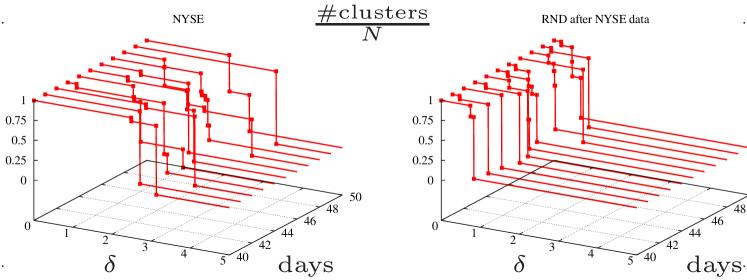
Figure 2: Typical behavior of the ratio of the number of distinct clusters to the total number of particles, versus connectivity distance $\delta$ for 10 different consecutive trading days. The left panel corresponds to real market data, and the right panel to the random surrogates sharing the same statistical properties.

We have determined $g(r)$ from a daily stock market data taken among 2784 equities traded in the New York Stock Exchange (NYSE) in the period between 01-Jan-1987 and 31-Dec-1998 (3032 trading days). To maintain a continuity of quotation, we have selected the maximal subset of 561 assets which, in the above mentioned period, remained consecutively traded. The associated pair potential $u(r)$ is shown in Fig. 1. It displays a long linear tail at large $r$ (of slope $=0.419\pm 0.001$, and correlation coefficient$=0.9998$ calculated over 116 points in the region $2.5<r<6$), indicating a remarkable long range character of the asset–asset interaction potential. These results are consistent with a previous calculation for a by far smaller set of stocks within the german DAX index [5].

We would like to learn next about the spatial heterogeneities in the $N$ particle system. One way to do this is to study the ‘clustering’ of particles, in a similar fashion as done in the description of clusters in percolation models [7]. In this case, particles are assumed to be connected to each other if their distance is smaller than some ‘connectivity distance’, $\delta$. The value of $\delta$ can be varied from $0$ to the linear size of the whole system, $S$. In the case of $\delta\ll S$, the particles are clearly disconnected and one finds $N$ single clusters. By increasing $\delta$ a first cluster is formed at a value $\delta_{\rm intra}$ giving a measure of the particle distance within the first formed cluster. When $\delta\to S$, all particles are connected to each other and a single cluster exists, and let $\delta_{\rm inter}$ denote the threshold to the formation of only one cluster. For intermediate values of $\delta$, the number of clusters decreases as $\delta$ increases. In the case of a homogeneous particle distribution in space, one expects to find a sort of critical value above which the number of clusters decreases rapidly when $\delta$ is increased. In other words, a cluster of connected particles ‘percolates’ the system. However, if the system is heterogeneous the transition may become quite different than in the homogeneous case. First results, obtained for a further subset of 67 NYSE stocks in the case of $H=2$ (daily and weekly horizons), suggest that the particle system is arranged in a sort of hierarchical fashion, in which small clusters are contained within larger ones. This is easily seen in Fig. 2. The ratio of the number of distinct clusters to the total number of particles is clearly time dependent, alternating homogeneous and heterogeneous phases. As a comparison, we have generated a surrogate data set by calculating at any time step the ellipse containing real market data in the embedding space. Its axes are the standard deviations of the fitting two–dimensional gaussian probability out of which we have drawn the surrogate data. It is worth saying that, as a result, every single surrogate stock shows the stylized facts of single asset finance (fat tails, volatility clustering etc.) but inexorably looses asset–asset correlation information.

To capture the basic features of the staircase plot of Fig. 2, we have calculated the extention of its non trivial plateaux $L=\delta_{\rm inter}-\delta_{\rm intra}$, and its number of jumps $n$ (Fig. 3).

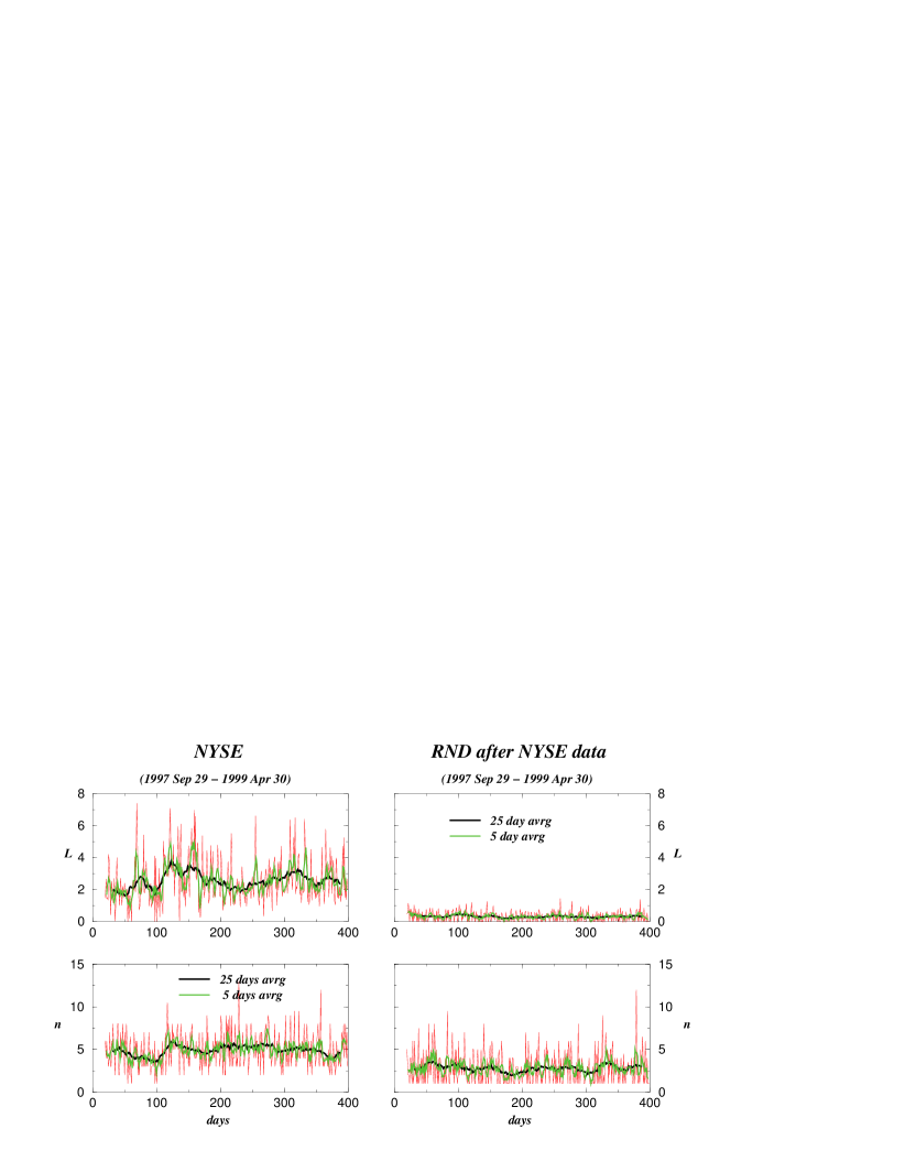
Figure 3: The length of the plateux $L$ and the number of jumps $n$ of the clustering curves are depicted for both real and random market data as in Fig. 2.

Market data and random data show markedly different behaviors. Averaged market data result in a richer structure due to the presence of a great hierarchy of clusters at different length scales (greater values of $n$). Moreover, at any length scale real market clusters are also spatially better separated (greater values of $L$). The strong time dependence of these indicators suggests that a clustering analysis which consider a behavior on long time scales may only give ‘average’ answers, missing the highly non–persistent dynamics of cluster particles.

To conclude, we have shown that a many asset market shows well marked indication of the correlations among assets. The asset–asset potential and the hierarchical time dependent cluster structures may reveal new paradigms for financial markets. The same analysis has been applied to a set of $N$ artificial prices generated with an agent based model (for traders with finite cash, picking stocks at random). It comes out that, despite individual stocks prices satisfy typical single asset empirical properties, the calculated collective indicators presented here are in significant disagreement with real market results [8].

We would like to thank to F. Lillo and R. Mantegna for providing daily data of equities traded in the NYSE. Fruitful discussions with Wolfgang Breymann are also acknowledged.

References

- [1] A.W. Lo, Econometrica 59 (1991) 1279–1313.
- [2] R.N. Mantegna and H.E. Stanley, An Introduction to Econophysics: Correlations and Complexity in Finance (Cambridge University Press, Cambridge, 1999).
- [3] W.A. Brock, W.D. Dechert, B.D. LeBaron and J.A. Scheinkman, Econometric Reviews 15 (1996) 197–235.
- [4] E.F. Fama, Journal of Financial Economics 49 (1998) 283–306.
- [5] G. Cuniberti and L. Matassini, To appear in The European Physical Journal B (2001). cond-mat/0101143.
- [6] J.-P. Hansen, I. R. McDonald, Theory of Simple Liquids (2nd Ed., Academic Press, 1986).
- [7] G. Grimmett, Percolation (Springer Verlag, 1999)
- [8] F. Castiglione, private communication.