Memory effects in vibrated granular systems

Abstract

Granular materials present memory effects when submitted to tapping processes. These effects have been observed experimentally and are discussed here in the context of a general kind of model systems for compaction formulated at a mesoscopic level. The theoretical predictions qualitatively agree with the experimental results. As an example, a particular simple model is used for detailed calculations.

1 Introduction

A granular material is a system composed of a “large” number of macroscopic particles or grains whose interactions are inelastic, so that mechanical energy is not conserved. Here, in practice, large means in many cases a few thousands or even hundreds of particles, as opposite to usual molecular systems having a number of particles of the order of Avogadro’s number. The macroscopic size of the particles implies that the usual concepts of thermodynamics can not be directly translated to these systems. For instance, if we consider a typical granular system such as sand, the energy needed to lift a grain by one diameter is more than ten orders of magnitude larger than the thermal energy of the grain at room temperature. Moreover, due to the inelasticity of collisions it is necessary to supply external (nonthermal) energy to the system in order to generate a steady state or to study the relaxation of the system towards a stable configuration. Therefore, although the concept of granular temperature is often used in the literature, it must be understood just as a measure of the velocity fluctuations in the system, without being related with any underlying idea of thermal equilibrium.

The phenomenology of granular media is very rich, showing many characteristic complex behaviours [1]. Here we will focus in one them, namely compaction, that can be roughly defined as the nonthermal relaxation of a loosely packed system of many grains under vertical mechanical tapping or vibration. This problem is of fundamental importance to many industrial applications and also raises fundamental theoretical questions. Therefore, it is not surprising that in the last years systematic experimental investigations and theoretical approaches are being developed to described the dynamics of compaction processes, as well as the nature of the final state reached by the system.

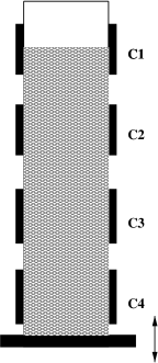
Figure 1: Sketch of the experimental set-up used in Reference [2]. The density is measured at four different heights by means of the capacitors $C1-C4$.

The evolution of the density in vibrated granular materials was investigated in a pioneering paper by Knight et al[2, 3]. The experimental set-up they used consisted of monodisperse spherical glass beads in a long thin cylinder mounted vertically on a vibration exciter. The packing fraction of the beads was measured by means of four capacitors mounted at different heights along the tube (see Figure 1). The shaking intensity $\Gamma$, determined by the maximum applied acceleration normalized by gravity, was controlled. The system was prepared in a low density initial state before being submitted to a sequence of single shakes or “taps”. Time between taps was long enough to allow the system to come to rest, so they were completely independent and internal resonances were avoided. It was observed that the density increased monotonically, tending eventually to a steady value. The number of taps required to reach the final density was very large, often larger than $10^{5}$.

The authors found that a good description of the experimental data was obtained with an inverse logarithm four parameter fit of the form

$$\rho(t)=\rho_{\infty}-\frac{\Delta\rho_{\infty}}{1+B\ln(1+t/t_{c})}\,,$$ (1)

where time is measured in number of taps and the parameters $\rho_{\infty}$, $\Delta\rho_{\infty}$, $B$, and $t_{c}$ are constants that depend only on the tapping strength $\Gamma$. The above inverse logarithmic expression fitted the data better than other more usual laws such as a single exponential, a combination of two exponentials, a power law, or a stretched exponential. Two features of the experimental results that are relevant for the later discussion here are

1. The slope of the relaxation curve is smaller for smaller vibration intensity $\Gamma$, i.e. the relaxation is slower for smaller $\Gamma$.

2. The final steady density is a monotonic decreasing function of $\Gamma$ [4].

A theoretical attempt to formulate a “thermodynamic” description of the steady states reached by the system in the long time limit has been carried out by Edwards and coworkers [5, 6, 7]. They extended the methods and concepts of usual statistical physics to granular media. The basic idea is that the volume plays in these systems a role analogous to that played by the energy in molecular (elastic) systems. Although there is no experimental verification of this theory up to now, it has been shown to be consistent with the behaviour of some simple models for granular compaction [8, 9, 10].

In addition to the slow relaxation described above, vibrated granular materials exhibit a series of properties that are reminiscent of the typical behaviour of conventional structural glasses. This includes effects as annealing, i.e. slow “cooling” properties, and hysteresis, when submitted to processes in which the tapping intensity is monotonically increased and decreased [3, 11]. This apparent glassy nature of granular compaction led Josserand et al[12] to investigate the response of a vibrated granular system to sudden perturbations of the intensity $\Gamma$. Their work was suggested by classical experiments for the study of aging in glasses, and the realization that the vibration intensity plays in vibrated granular media a role analogous to the temperature of molecular systems. Previously, a similar process had been studied by means of numerical simulations in a model for compaction [13].

In the simplest compaction experiment of Reference [12], the vibration intensity was instantaneously changed from a value $\Gamma_{1}$ to another $\Gamma_{2}$ after $t_{w}$ taps. For $\Gamma_{1}>\Gamma_{2}$ it was observed that on short times scales the compaction rate increases, while for $\Gamma_{2}>\Gamma_{1}$ the system dilates for short times. Both results are opposite from the behaviour at constant $\Gamma$, as discussed above. After several taps, the “normal” behaviour was recovered. This is a direct evidence of the presence of short-term memory effects in the system, so that the density for $t>t_{w}$ is not determined by its value at $t=t_{w}$. Other experiments are also reported by the authors showing the same kind of non-Markovian behaviour. In the next section we will investigate whether this anomalous response can be understood in terms of simple and general arguments.

2 Mesoscopic description of the density evolution

When a granular system is being vibrated, different kind of events take place in the system. The existence of a steady density for constant vibration intensity suggests the presence of two different kinds of elementary processes, the ones trying to increase the density and the others trying to decrease it. Stationarity arises when both tendencies cancel each other. Then, we will assume that the time evolution of the density $\rho$ in a tapping process can be described at a mesoscopic level by a balance equation of the form

$$\frac{d\rho(t)}{dt}=f_{1}(\Gamma)\mu_{1}(t)-f_{2}(\Gamma)\mu_{2}(t),$$ (2)

where $t$ is measured in number of taps, and the several functions verify

$$f_{1}(\Gamma)\geq 0,\quad f_{2}(\Gamma)\geq 0,$$ (3)

$$\mu_{1}(t)>0,\quad\mu_{2}(t)>0.$$ (4)

The quantities $\mu_{1}(t)$ and $\mu_{2}(t)$ are assumed to include all the correlation effects. Note that we do not assume that $\mu_{1}$ and $\mu_{2}$ can be expressed as functions of $\rho(t)$, so that Equation (2) is not closed. Our aim in the following will be to investigate what information can be obtained about $f_{1}$, $f_{2}$, $\mu_{1}$, and $\mu_{2}$ by using very general and plausible physical arguments. First, we notice that since we are measuring the time in units of complete taps, if there is no tapping there is no time evolution either. Therefore, it must be

$$f_{1}(\Gamma=0)=f_{2}(\Gamma=0)=0.$$ (5)

Moreover, the number of elementary processes, both tending to increase and to decrease the density, are expected to increase with $\Gamma$. This expectation is reinforced by the analogy of $\Gamma$ with the temperature, as mentioned in the previous section. Then we assume that $f_{1}(\Gamma)$ and $f_{2}(\Gamma)$ are both monotonic increasing functions. Let us introduce the function

$$g(\Gamma)\equiv\frac{f_{2}(\Gamma)}{f_{1}(\Gamma)}\,,$$ (6)

representing the ratio of the rate associated to the decompaction processes to that of the compaction ones. As already mentioned, experiments show that the steady density is a decreasing function of $\Gamma$. This suggests that $g(\Gamma)$ must be an increasing function of the vibration intensity, so that decompaction events become relatively more relevant. This assumption can be further justified by analysing the behaviour of the steady solutions of Equation (2) [14]. Then we can rewrite our mesoscopic evolution equation as

$$\frac{d}{dt}\rho(t)=f_{1}(\Gamma)\left[\mu_{1}(t)-g(\Gamma)\mu_{2}(t)\right].$$ (7)

Here $f_{1}(\Gamma)$, $g(\Gamma)$, $\mu_{1}(t)$, and $\mu_{2}(t)$ are all positive quantities. Moreover, the first two ones are increasing functions of $\Gamma$, vanishing in the limit $\Gamma\rightarrow 0$. This fully specifies the general kind of evolution equations we will deal with. Let us consider the following experiment. A system is vibrated with a constant intensity $\Gamma$. At a given time $t_{w}$, the intensity is instantaneously changed to $\Gamma+\Delta\Gamma$. We want to study the change in the relaxation rate $r(t)\equiv d\rho(t)/dt$. Just before the change we get from (7),

$$r_{w}=f_{1}(\Gamma)\left[\mu_{1}(t_{w}^{-})-g(\Gamma)\mu_{2}(t_{w}^{-})\right],$$ (8)

while just after the change it is

$$r_{w}^{\prime}=f_{1}(\Gamma+\Delta\Gamma)\left[\mu_{1}(t_{w}^{+})-g(\Gamma+\Delta\Gamma)\mu_{2}(t_{w}^{+})\right].$$ (9)

Then, for $\Delta\Gamma\ll 1$, we get

$$\frac{\Delta r_{w}}{\Delta\Gamma}\equiv\frac{r^{\prime}_{w}-r_{w}}{\Delta\Gamma}=\lambda(t_{w}),$$ (10)

where we have defined the function ($r(t)$ and $\mu_{2}(t)$ are computed over the relaxation curve at constant $\Gamma$)

$$\lambda(t)=\frac{f^{\prime}_{1}(\Gamma)}{f_{1}(\Gamma)}r(t)-f_{1}(\Gamma)g^{\prime}(\Gamma)\mu_{2}(t).$$ (11)

Upon deriving Eq. (10) we have assumed that $\mu_{1}(t)$ and $\mu_{2}(t)$ are continuous at $t=t_{w}$. This seems physically plausible since they are functionals of the state of the system. For instance, in the mesoscopic description they can be expressed as given moments of the underlying distribution function of the system, which is known to be a continuous function of time. In the limit $t_{w}\rightarrow\infty$, the system has time to reach the stationary density corresponding to the intensity $\Gamma$ before the change, so that $r_{w}=0$ and $\lambda(t_{w})<0$, because of the properties of the functions $f_{1}(\Gamma)$ and $g(\Gamma)$. In the opposite limit, $t_{w}\rightarrow 0$, and assuming that the initial density is close to its minimum value, it is $\lambda(t_{w})>0$. To derive this, we have taken into account that $\mu_{2}$ must vanish in the lowest density limit, where by definition no processes decreasing the density are possible. The conclusion of this discussion is that $\lambda(t_{w})$ has opposite signs in the short and large $t_{w}$ limits. Then, it follows from Eq. (10) that when the system has been vibrated for a short time before the change of vibration intensity, $\Delta r_{w}$ and $\Delta\Gamma$ have the same sign, i.e. the response of the system is what we have described in the previous section as normal. On the other hand, if the vibration time before the change is large, the response of the system is anomalous. In this context, the experiments reported in Reference [12] would correspond to “large” vibrating periods before the abrupt change in the shaking intensity.

3 A simple model for granular compaction

In this Section we are going to describe a one-dimensional model for granular compaction [15] that is simple enough as to allow for detailed calculations, and at the same time captures many of the experimental characteristic features. We consider a lattice in which each site $i$ can be either occupied by a particle or empty (occupied by a hole). A variable $m_{i}$ is assigned to each site, taking the value $m_{i}=1$ if the site is empty, and $m_{i}=0$ if there is a particle on it. The time evolution of the system is defined in the following way. The only possible elementary events occurring in the system are the adsorption of a particle on an empty site and the desorption of a particle from the lattice to the bulk. Then the dynamics is formulated by means of a master equation with a transition rate for the change of $m_{i}$ into $1-m_{i}$ given by

$$W_{i}({\bf m})=\frac{\nu}{2}(m_{i-1}+m_{i+1})\left[\epsilon+m_{i}(1-2\epsilon)\right].$$ (12)

Here ${\bf m}\equiv\{m_{1},m_{2},\ldots\},$ $\nu$ is a frequency defining the characteristic time scale, and $\epsilon$ is a dimensionless parameter taking values in the interval $0\leq\epsilon\leq 1$. Thus the transition rate for the adsorption of a particle at site $i$ is

$$W_{i}^{+}({\bf m})=\frac{\nu}{2}(1-\epsilon)m_{i}(m_{i-1}+m_{i+1}),$$ (13)

and that for the desorption of a particle

$$W_{i}^{-}({\bf m})=\frac{\nu}{2}\epsilon(1-m_{i})(m_{i-1}+m_{i+1}).$$ (14)

It is seen that for $\epsilon=1$ no particle can be absorbed, while for $\epsilon=0$ desorption processes are inhibited. Moreover, all processes are restricted, in the sense that a site can change its state only if at least one of its nearest neighbour sites is empty. A similar kind of facilitated dynamics has been considered in the formulation of Ising models for glassy relaxation [16]. A physical picture of the model can be obtained by associating a hole with a region of the granular system having a low density, and a site occupied by a particle with a high density region. The facilitated dynamics tries to translate the idea that fluctuations leading to rearrangements in a region require a neighbour region with low packing fraction. Our one-dimensional model is a very idealized representation of a low horizontal layer in a vibrated granular system, the parameter $\epsilon$ being related with the intensity of vibration.

In order to model a tapping experiment, the system is initially placed in a purely random configuration, from which it relaxes with $\epsilon=0$ until it gets eventually trapped in a metastable state, with all the holes surrounded by two particles. This is a low density configuration that is taken to correspond to the loosely initial conditions used in real experiments. Then, a pulse is generated by instantaneously increasing $\epsilon$ to a given value for a time period $t_{0}$. Afterwards, the system relaxes again with no external excitation, i.e. with $\epsilon=0$. In order to mimic what is done in experiments, the relaxation lasts long enough as to allow the system to reach a metastable configuration, from which no evolution is possible in absence of external excitation. This completes a tap event. The process is repeated to generate a series of them.

A first test of the relevance of the model to study compaction in vibrated granular systems is, of course, whether it leads to the same kind of density evolution at constant vibration intensity as experimentally observed. We have verified that this is the case in the limit $\epsilon\nu t_{0}\ll 1$. The mean density in an homogenous configuration is given by $\rho(t)\equiv 1-\langle m_{i}(t)\rangle$, with the angular brackets denoting ensemble average and $i$ being arbitrary.

Figure 2: Time evolution of the density of the model described in the main text when it is submitted to a tapping process with $\epsilon=0.5$. Data obtained with three different values of $t_{0}$, namely $0.002$, $0.001$, and $0.02$ have been plotted.

An example is given in Figure 2, where the relaxation of the density is plotted as a function of the scaled time $\tau_{n}=\nu\epsilon t_{0}n$, $n$ being the number of taps. The numerical data have been obtained from Monte Carlo simulations and different values of $\epsilon$ and $t_{0}$ have been used. The fact that all curves collapse indicates that $\tau_{n}$ is the relevant time scale for the compaction problem. Also plotted in the same figure is the fit to the phenomenological law (1), with parameters $\rho_{\infty}=1.10$, $\Delta\rho_{\infty}=0.40$, $B=0.39$, and $t_{c}=3.37/\nu\epsilon t_{0}$. It is seen that the inverse logarithmic law describes very well the simulation results. A similar behaviour has also been found in other models for granular compaction [17, 18, 19]. Nevertheless, we ought to say that we have not been able to derive the heuristic relaxation law by analytical methods, in spite of the tractability of our model. It is possible that it be just a convenient fitting expression over a wide time window. A strong indication supporting this idea is that the steady density predicted by the logarithmic law $\rho_{\infty}$ in the limit of an asymptotically large number of taps not only is in disagreement with the simulations, but is clearly unphysical since it is larger than one. The same happens with the experimental results, where $\rho_{\infty}$ is sometimes greater than the random close packing [2]. In fact, it is possible to derive an analytical expression for the asymptotic density reached by the model with the result

$$\rho_{0}^{(s)}\simeq 1-\frac{1}{2}\epsilon\nu t_{0},$$ (15)

valid again in the limit $\epsilon\nu t_{0}\ll 1$. Also this expression has been checked by Monte Carlo simulations [15].

4 Effective dynamics for tapping processes

Figure 3: The effective dynamics tries to define the transitions between the crosses, which correspond to the results of the successive taps.

The stochastic model formulated in the previous section, with the transition rates given by Eq. (12), can be used to study a variety of compaction processes by specifying the time dependence of the control parameter $\epsilon$. In particular, we have already discussed some applications to tapping processes, based on the particularization of the general equations following from the master equation to a specific way of vibrating the system. A different, and more appealing, approach is to look for an effective master equation following from (12) and being appropriated for a given experiment. We have developed such a program for tapping processes [8]. The idea is to look for effective transitions rates, $W_{ef}({\bf m}|{\bf m}^{\prime})$, connecting the initial and final states of the system when it is submitted to a “elementary event” (see Figure 3). The latter is defined as the combination of a tap and the posterior free relaxation to a metastable configuration. In the limit of $\epsilon\nu t_{0}\ll 1$, three groups of possible transitions are identified:
a)Elementary diffusive events, conserving the number of particles. They correspond to the interchange of a hole and a particle,

$$\ldots 100\ldots\rightarrow\ldots 010\ldots,\\ \ldots 001\ldots\rightarrow\ldots 010\ldots.$$ (16)

The effective transition rate for each of these processes is $\alpha/2$, where

$$\alpha=\frac{\nu t_{0}\epsilon}{2}.$$ (17)

is a positive constant playing a role similar to that played by $\Gamma$ in the real experiments.
b)Transitions increasing the number of particles. There are three of them,

$$\ldots 101\ldots\rightarrow\ldots 010\ldots,$$ (18)

with transition rate $\alpha/2$,

$$\ldots 101\ldots\rightarrow\ldots 001\ldots,$$ (19)

with transition rate $\alpha/4$, and

$$\ldots 101\ldots\rightarrow\ldots 100\ldots,$$ (20)

also with transition rate $\alpha/4$.
c)Transitions decreasing the number of particles. These are

$$\ldots 00100\ldots\rightarrow\ldots 01010\ldots,$$ (21)

with transition rate $\alpha^{2}/2$ and

$$\ldots 01000\ldots\rightarrow\ldots 01010\ldots,$$ (22)

$$\ldots 00010\ldots\rightarrow\ldots 01010\ldots,$$ (23)

both with $W_{ef}=\alpha^{2}/4$. Only those variables corresponding to sites whose state is changing or conditioning the transition are represented in the above expressions. The equivalence of this model to the original one defined by the transition rates (12) in the limit of small $\alpha$, has been tested by comparing the Monte Carlo simulation results obtained with both models. In fact, the data show that, for the density relaxation, the results from the effective model and the original one differ by less than $2$ per cent for $\alpha\leq 0.5$. For constant $\alpha\neq 0$, the system evolves from the initial low density configuration to a final state characterized by a density

$$\rho_{s}(\alpha)=\frac{1}{2}\left[1+\left(1+4\alpha\right)^{-1/2}\right].$$ (24)

Figure 4: Evolution of the density when the system is submitted to a tapping cycle as described in the text. The diamonds and the crosses represent the approximately reversible cooling and heating processes, respectively.

A detailed analysis of the properties of the steady state [8] shows that they are consistent with Edwards’s theory [5, 6, 7], with the compactivity being identified as $X=-(\ln\alpha)^{-1}$. Furthermore, when the system described by the effective transition rates is submitted to processes in which the tapping intensity is first monotonically increased and afterwards decreased also monotonically, its time evolution presents the reversible-irreversible branches observed in experiments [20]. In Figure 4 an example of the response of the system to one of these cycles is presented. The compactivity $X$ of the system is decreased and increased with the same rate, $r=10^{-5}$. Starting from the loosest configuration, for large enough vibration intensity (or compactivity) the density of the system approaches the steady curve. Afterwards, when the compactivity is decreased and increased, always with the same rate, two (approximately) reversible curves are obtained. These hysteresis effects are related with the existence of a “normal evolution curve”, fully determined by the program of increase of the intensity, and having the strong property of attracting any other solution of the master equation with the same program [20].

5 Memory effects

Now, we will show that the effective dynamics introduced above leads to a model for tapping processes that belongs to the general class discussed in Section 2 and, consequently, also presents the short term memory effects observed in vibrated granular materials. We start by noting that the steady density for constant intensity, given by (24) is a monotonic decreasing function of $\alpha$, going from $\rho_{max}=1$ to $\rho_{min}=0.5$. Next, from the master equation with the transition rates (16)-(23) it is obtained

$$\frac{d\rho}{dt}=\alpha x_{101}(t)-\frac{\alpha^{2}}{2}\left[x_{00100}(t)+\frac{1}{2}x_{01000}(t)+\frac{1}{2}x_{00010}(t)\right],$$ (25)

where $x_{101}$ is the concentration of hole-particle-hole clusters, $x_{00100}$ is the concentration of two particles-hole-two particles clusters, and so on. Comparison of the above equation with (7) shows that both equations have the same form, with the choices

$$f_{1}(\alpha)=g(\alpha)=\alpha,$$ (26)

$$\mu_{1}(t)=x_{101}(t),\quad\mu_{2}(t)=\frac{1}{2}x_{00100}(t)+\frac{1}{4}\left[x_{01000}(t)+x_{00010}(t)\right].$$ (27)

Since $f_{1}$ and $g$ are monotonic increasing functions of $\alpha$, and $\mu_{1}$ and $\mu_{2}$ are defined positive quantities, the model verifies the conditions required by the validity of the discussion carried out in Section 2. Therefore, we can directly write from Eq. (10)

$$\frac{\Delta r_{w}}{\Delta\alpha}=\lambda(t_{w}),$$ (28)

where the function $\lambda(t)$ determining the nature of the response of the system is

$$\lambda(t)=\frac{r(t)}{\alpha}-\alpha\mu_{2}(t).$$ (29)

For instance, for $\alpha=0.15$, Monte Carlo simulations show that $\lambda(t)>0$ for $t<t_{c}$, while $\lambda(t)<0$ for $t>t_{c}$, with $19<t_{c}<20$ [14]. According to the theory presented here, when the vibration intensity $\alpha$ is modified at a time $t_{w}<t_{c}$, a normal response in which the intensity jump and the relaxation rate jump have the same sign is to be expected. On the other hand, when $t_{w}>t_{c}$, stimulus and response should have opposite signs, corresponding to an anomalous response. In Figure 5 we have plotted the time evolution of the density of a system which is being vibrated with $\alpha=0.15$, and the intensity is suddenly decreased to $\alpha=0.125$ at $t=t_{w}$. The only difference between the two curves is in the value of $t_{w}$; in one case it is $t_{w}=10<t_{c}$ while in the other $t_{w}=50>t_{c}$. In agreement with the theoretical analysis, the relaxation rate at the jump decreases in the first case and increases in the latter.

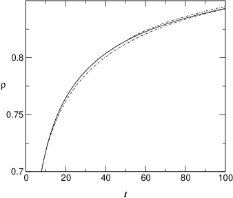
Figure 5: Response of the system to a sudden change in the vibration intensity from $\alpha=0.15$ to $\alpha=0.125$. When the jump is introduced at $t_{w}=10<t_{c}$, the response is normal, i.e. the slope of the relaxation curve decreases. On the other hand, for $t_{w}=50>t_{c}$ an anomalous response is observed.

It is important to stress the generality of the arguments in Section 2. Although we have restricted ourselves in this work to a particular simple model of compaction, the theoretical scheme presented there is rather general. For instance, an equation like (7) is also found for the so-called parking model [19, 21]. Even more, the one-dimensional Ising model with Glauber dynamics also belongs to the group [22]. In summary, the memory effects discussed in the context of compaction in granular materials seem to be quite general effects showing up in many different systems.

References

References

- [1] Jaeger H, Nagel S R, Behringer R 1996 Rev. Mod. Phys. 68 1259
- [2] Knight J B, Fandrich C G, Lau C N, Jaeger H M, and Nagel S R 1995 Phys. Rev. E 51 3957
- [3] Nowak E R, Knight J B, Ben-Naim E, Jaeger H M, and Nagel S R 1998 Phys. Rev. E 57 1971
- [4] The insert in Figure 5 of Reference [2] can be misleading, since the parameter shows there an increasing behaviour with . Nevertheless, this is due to the fact that the states considered for small values of do not correspond to the final stable configuration, but to metastable ones [3]
- [5] Edwards S F and Oakeshott R B S 1989 Physica A 157 1080
- [6] Mehta A and Edwards S F 1989 Physica A 157 1091
- [7] Edwards S F and Mounfield 1994 Physica A 210 279
- [8] Brey J J, Prados A, and Sánchez-Rey B 2000 Physica A 275 310
- [9] Lefevre A and Dean D S 2001 J. Phys. A: Math. Gen. 34 L213; Dean D S and Lefevre A 2001 Phys. Rev. Lett. 86 5639
- [10] Barrat A, Kurchan J, Loreto V, and Sellitto M 2000 Phys. Rev. Lett. 85 5034; 2001 Phys. Rev. E 63 051301
- [11] Jaeger H M 1998 Physics of Dry Granular Media ed H J Herrmann et al(Dordrecht: Kluwer Academic) p 553
- [12] Josserand C, Tkachenko A, Mueth D M, and Jaeger H M 2000 Phys. Rev. Lett 85 3632
- [13] Nicodemi M. 1999 Phys. Rev. Lett 82 3734
- [14] Brey J J and Prados A 2001 Phys. Rev. E 63 061301
- [15] Brey J J, Prados A, and Sánchez-Rey B 1999 Phys. Rev. E 60 5685
- [16] Fredrickson G H and Andersen H C 1984 Phys. Rev. Lett. 53 1244; 1985 J. Chem. Phys. 83 5822
- [17] Caglioti E, Loreto V, Herrmann H L, and Nicodemi M 1997 Phys. Rev. Lett. 79 1575
- [18] Nicodemi M, Coniglio A, and Herrmann H J 1997 Phys. Rev. E 55 3962
- [19] Ben-Naim E, Knight J B, Nowak E R, Jaeger H M, and Nagel S R 1998 Physica D 123 380
- [20] Prados A, Brey J J, and Sánchez-Rey B 2000 Physica A 284 277
- [21] Kraprivsky P L and Ben-Naim E 1994 J. Chem. Phys. 100 6778
- [22] Brey J J and Prados A 2001 Europhys. Lett. (in press); e-print cond-mat/0105232