Nonstandard mixing in the standard map

Abstract

The standard map is a paradigmatic one-parameter (noted $a$) two-dimensional conservative map which displays both chaotic and regular regions. This map becomes integrable for $a=0$. For $a\neq 0$ it can be numerically shown that the usual, Boltzmann-Gibbs entropy $S_{1}(t)=-\sum_{i}p_{i}(t)\ln{p_{i}(t)}$ exhibits a linear time evolution whose slope hopefully converges, for very fine graining, to the Kolmogorov-Sinai entropy. However, for increasingly small values of $a$, an increasingly large time interval emerges, before that stage, for which linearity with $t$ is obtained only for the generalized nonextensive entropic form $S_{q}(t)=\frac{1-\sum_{i}[p_{i}(t)]^{q}}{q-1}$ with $q=q^{*}\simeq 0.3$. This anomalous regime corresponds in some sense to a power-law (instead of exponential) mixing. This scenario might explain why in isolated classical long-range $N$-body Hamiltonians, and depending on the initial conditions, a metastable state (whose duration diverges with $1/N\rightarrow 0$) is observed before it crosses over to the BG regime.

PACS numbers: 05.20.-y, 05.45.-a, 05.70.Ce

In his critical remarks about the domain of validity of Boltzmann principle, Einstein stressed [1] that the basis of statistical mechanics lies on dynamics. Intensive work has recently been done which is consistent with this standpoint, specifically in situations where anomalous effects may arise ([2, 3, 4, 5, 6, 7]). Also, a particularly interesting observation was made in [8], where it was found a simple connection between the Kolmogorov-Sinai (KS) entropy rate (the one that stems from the properties of mixing of the system) and the statistical entropy (the one that originates from a probability distribution). It was shown in fact that, partitionning the phase space in $W$ cells and starting from many points within one cell, the time dependence of the usual, Boltzmann-Gibbs (BG), statistical entropy

$$S_{1}=-\sum_{i=1}^{W}p_{i}\ln{p_{i}},$$ (1)

includes a linear stage whose slope coincides with the KS entropy rate, calculated, via Pesin equality, using the Lyapunov exponents. Finally, for one-dimensional dissipative systems at the edge of chaos (e.g., the logistic map), it was found in [7] that the usual entropy fails to exhibit (with nonvanishing slope) such a behavior. Instead, the nonextensive entropy [9] (for a recent review, see [10])

$$S_{q}=\frac{1-\sum_{i=1}^{W}p_{i}^{q}}{q-1},$$ (2)

succeeds for a specific value of $q<1$ ($q^{*}\simeq 0.2445$ for the logistic map). We remind that the entropic form (2) reduces to (1) in the limit $q\rightarrow 1$ and that its extremum at equiprobability ($p_{i}=1/W,\;\;\forall i$) is given by $S_{q}=(W^{1-q}-1)/(1-q)$.

In Hamiltonian dynamics, one of the most studied models is the standard map (see, for instance, [11]), also referred to as the kicked-rotator model:

$$x_{t+1} = y_{t}+\frac{a}{2\pi}\sin(2\pi x_{t})+x_{t}~{}~{}~{}\textup{(mod 1)},$$

$$y_{t+1} = y_{t}+\frac{a}{2\pi}\sin(2\pi x_{t})~{}~{}~{}~{}~{}~{}~{}~{}~{}\textup{(mod 1)},$$

where $a\in\mathbb{R}$. It corresponds to an integrable system when $a=0$, while, for large-enough values of $a$ (typically $|a|\geq 7$), the map is strongly chaotic . It can be easily verified that, for all values of $a$, this two-dimensional map is conservative; it has a pair of $(x,y)$-dependent Lyapunov exponents, which only differ in sign (simplectic structure) and globally vanish when $a$ vanishes.

In this letter we study the time evolution of both the extensive ($q=1$) and the nonextensive ($q\neq 1$) statistical entropies of the standard map (Nonstandard mixing in the standard map), focusing our attention on small values of the parameter $a$, i.e., on those situations where the border between the chaotic and the regular regions has a relevant influence. For decreasingly small values of $|a|$ below say $7$, one encounters in fact an increasingly rich fractal-like structure, characteristic of a large class of Hamiltonian systems. Typically, chains of regular islands corresponding to elliptic points in resonance condition begin to appear, and between each couple of elliptic points of a chain there is an hyperbolic point, thus forming another chain of hyperbolic points responsible for the chaotic areas. Around each island there is another chain of islands of a higher order and, once again, another chain of hyperbolic points between the islands (see, for instance, [12] for details). This structure is usually referred to as “islands-around-islands”. If in some sense we think at the islands-around-islands structure as the edge-of-chaos region of a Hamiltonian system, we verify that for the standard map its relative area of influence increases if $a$ approaches $0$.

We know from the theory of chaos that the mixing (herein we use this word as a synonym of sensitivity to initial conditions: $\xi(t)\equiv\lim_{\Delta x(0)\to 0}\Delta x(t)/\Delta x(0)$, for a one-dimensional illustration), is typically linear ($\xi-1\propto t$) in the case of a regular region, and exponential in the case of a strongly chaotic one ($\dot{\xi}=\lambda_{1}\xi$, hence $\xi=e^{\lambda_{1}t}$, with the Lyapunov exponent $\lambda_{1}>0$). When a point falls in the neighborhood of the islands-around-islands structure, it becomes trapped, a phenomenon called “stickiness” (see, for instance, [13]); its motion may be thought in this case as a succession of “flights and sticks”. We suggest here, on the basis of the results that follow, that the presence of the fractal-like structure at the border between regular and strongly chaotic regions produces a power-law mixing of the kind ([2]):

$$\xi=e_{q^{*}}^{\lambda_{q^{*}}t}\equiv\left[1+(1-q^{*})\lambda_{q^{*}}t\right]^{\frac{1}{1-q^{*}}}$$ (4)

(see [10] for details on the $q$-exponential function), solution of the nonlinear equation $\dot{\xi}=\lambda_{q^{*}}\xi^{q^{*}}$, ($q^{*}<1$, $\lambda_{q^{*}}>0$). If we are then to construct a global solution $\xi(t)$, representative of the mixing properities of the whole phase space, we must implement some averaging process over regions with different kinds of mixing. In this case we expect that one or even two crossovers may happen when time increases, more precisely between the linear and the power-law mixings, and, later on, between the power-law and the exponential mixings. One way to model such a behavior is to assume that the differential equation that controls $\xi$ has the form [14] $\dot{\xi}=\lambda_{1}\xi+(\lambda_{q^{*}}-\lambda_{1})\xi^{q^{*}}$. The solution

$$\xi(t)=\left[1-\frac{\lambda_{q^{*}}}{\lambda_{1}}+\frac{\lambda_{q^{*}}}{\lambda_{1}}e^{(1-q^{*})\lambda_{1}t}\right]^{\frac{1}{1-q^{*}}},$$ (5)

presents, in the case $0<\lambda_{1}\ll\lambda_{q^{*}}$, three asymptotical behaviors, namely (i) linear ($q=0$ regime): $\xi\sim 1+\lambda_{q^{*}}t$, for $0\leq t\ll t_{cross1}\equiv\frac{1}{(1-q^{*})\lambda_{q^{*}}}$; (ii) power-law ($q=q^{*}$ regime): $\xi\sim\left[(1-q^{*})\lambda_{q^{*}}\right]^{\frac{1}{1-q^{*}}}t^{\frac{1}{1-q^{*}}}$, for $t_{cross1}\ll t\ll t_{cross2}\equiv\frac{1}{(1-q^{*})\lambda_{1}}$; (iii) exponential ($q=1$ regime): $\xi\sim(\frac{\lambda_{q}}{\lambda_{1}})^{\frac{1}{1-q}}e^{\lambda_{1}t}$, for $t\gg t_{cross2}$.

With this picture in mind, we explore now numerically the behavior of the entropy with time. We start introducing a coarse-graining partition of the mapping phase space by dividing it in $W$ cells of equal size, and we set many copies of the system ($M$ points) in a far-from-equilibrium situation putting all the $M$ points randomly or uniformly distributed inside a single cell. The occupation number $M_{i}$ of each cell $i$ ($\sum_{i=1}^{W}M_{i}=M$) provides a probability distribution $p_{i}\equiv M_{i}/M$, hence an entropy value. Using then the dynamic equations (Nonstandard mixing in the standard map), at each step the points spread in the phase space causing the entropy value to change. In order to obtain a numerically consistent definition of the probabilities $\{p_{i}\}$ when the system spreads at its maximum, we set $M>10\;W_{max}$, where $W_{max}\leq W$ is the maximum number of cells that the initial data occupy for the steps we are considering. Finally, to extract a global quantity on the $(x,y)$ phase space, we repeat the calculation setting the cell that contains the initial points in different positions chosen randomly all over the whole unit square, and we take an average over all the different histories thus obtained. We stress here that in taking this average all over the phase space we are consistent with a Gibbsian point of view, thus obtaining a statistical description of how the system approaches equilibrium. The result of this analysis for fixed $a$ is then a single curve of the entropy versus time, for each entropic form $S_{q}$.

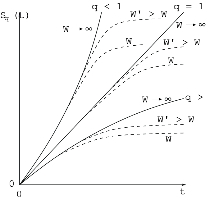
Figure 1: Schematic representation of $S_{q}(t)$ for different values of $q$, in the case of exponential mixing. Only for $q=1$ we have a finite entropy production ($\lim_{t\to\infty}S_{q}(t)/t$).

When the mixing is exponential and we use $q=1$, we obtain the behavior illustrated in [8]: a linear increase just before the saturation due to the finiteness of $W$, with a slope approaching, for $W\to\infty$, the positive Lyapunov exponent. If we vary $q$, we have that for $q<1$ $(q>1)$ the entropy grows with positive (negative) concavity before saturation. The exponential mixing is telling us that there is an unique value of $q$, namely $q=1$, which produces a linear growth in the entropy. We schematize this analysis in Fig. 1. Nevertheless, if some phenomenon like the trapping one described in [13] causes the mixing to slow down, thus becoming power-law, the same analysis exhibits that the only value of $q$ for which the entropy displays a linear stage with time is $q=q^{*}$, with $q^{*}<1$ (see, for example, [7]). Finally, if the mixing is linear, the specific value of $q$ corresponding to a linear stage is $q=0$.

In the case of the standard map the situation is more intricated because we have a coexistence of regions with different mixing properties. Fixing, for example, $a=5$, the phase space presents, macroscopically, two islands and a connected chaotic sea. Depending on where we set the initial data, we may face a strongly chaotic, or a regular, or even an islands-around-islands region. Our averaging procedure does not privilege any of these regions and allows the predominant one to emerge. The key point is to perform many different histories so that the average stabilizes on a definite curve. The resulting entropy curves are then sensible to two different phenomena: the characteristics of the mixing of each area (represented by the Lyapunov exponent $\lambda_{1}$, or its generalization $\lambda_{q^{*}}$ in the case of a power-law mixing) and the relative extension of each area with respect to the whole phase space (for this reason, in the following we indicate the slopes of the linear phases of $S_{q}(t)$ with $\widetilde{\lambda}_{q}$). If the phase space exhibits a predominance of power-law mixing region associated with a generalized Lyapunov exponent $\lambda_{q^{*}}$, with $q^{*}<1$, we expect, for time not too large, a linear growth for the entropy $S_{q^{*}}$. Waiting enough time, a crossover to the exponential mixing would occur, due to the rapidity of the exponential growth with respect to the power-law one, regardeless of how small is the exponential mixing region. After the crossover, the linearity with $t$ is obtained for $S_{1}$ (and not for $S_{q^{*}}$). We represent this more complex situation in Fig. 2, in the limit $W\to\infty$.

Let us present now our computational results for typical values of $a$. Fig. 3 represents the case $a=5$ and exhibits the predominance of the exponential-mixing. After the first step, that here and in what follows we consider as a transient, only the BG entropy $S_{1}(t)$ has a linear stage before the effects of saturation, while $S_{q}$ has positive concavity for $q=0.7$ and negative concavity for $q=1.3$. For $q=1$, our estimation of the slope $\widetilde{\lambda}_{1}(5)=0.96$ is different from that found in [8] because here we average all over the phase space, including the islands.

We notice that the scale that each entropic form covers, varies widely. To perform a linearity analysis between different entropy curves we use the following quite sensitive method. First, we fit the relevant piece of each curve (between $t=t_{1}$ and $t=t_{2}$) with a polynomial of the second degree: $At^{2}+Bt+C$. Then, we define the linearity coefficient $\rho\equiv A/(At_{2}^{2}+Bt_{2}-At_{1}^{2}-Bt_{1})$; $\rho$ tests the value of the second derivative of the fitting polynomial, including a scale renormalization. Obviously, $\rho=0$ corresponds to linearity, while $\rho>0$ and $\rho<0$ correspond to positive and negative curvatures respectively. An important remark is that the effect of saturation for a finite value of $W$ decreases the curvature of an entropy curve with respect to the case $W\to\infty$. This in turns introduces a systematic underestimation of $\rho$, which increases when $t_{1}$ and $t_{2}$ increase.

In Fig. 4 we show how, decreasing $a$, the first part of the $S_{1}(t)$ becomes concave. After the crossover the curves exhibit once again a linear increase. The slope of the linear stage becomes smaller, which suggests that the Lyapunov exponent $\lambda_{1}$ is globally going to $0$. In correspondence with the negative concavity of the first part of $S_{1}(t)$, $S_{0.3}(t)$ displays a linear increase (Fig. 5), with a slope that does not decrease as fast as the one of $S_{1}(t)$ (see the inset of Fig. 4). After the crossover, $S_{0.3}(t)$ becomes convex. We notice also that the crossover time $t_{cross}$ increases when $a$ decreases (inset of Fig. 5). It is the same linearity analysis performed in Fig. 3(d) which leads to $q^{*}\simeq 0.3$.

Summarizing, we have studied the production of entropy for a well known low-dimensional conservative map controlled by the parameter $a$. It appears that, for fixed $a\neq 0$ and in the limit $t\rightarrow\infty$ (to be in all cases taken after the $W\rightarrow\infty$ limit), it is the standard, BG entropy $S_{1}$, which is associated with a finite entropy production. However, during the time interval preceeding this extreme limit, an increasingly large interval emerges for which it is $S_{q^{*}}$, with $q^{*}\simeq 0.3$, which is associated with a finite entropy production. Consistently, our results suggest that, in the $lim_{t\rightarrow\infty}\;lim_{a\rightarrow 0}$ ordering, the only regime in fact observed is that corresponding to $q^{*}\simeq 0.3$. This fact provides a very appealing scenario for (meta) equilibrium thermostatistics in long-range Hamiltonians such as that considered in [15]. For these systems, a longstanding metastable state can exist (preceeding the BG one) whose duration diverges with $N\rightarrow\infty$, and whose distribution of velocities is not Maxwellian, but rather a power-law. The role played by $a$ in our present simple map and that played by $1/N$ in such long-range-interacting many-body systems, might be very similar, thus providing a dynamical basis for nonextensive statistical mechanics [9].

1 Acknowledgments

We acknowledge E.G.D. Cohen for stressing our attention on Einstein’s 1910 paper. We have benefitted from partial support by PRONEX, CNPq, CAPES and FAPERJ (Brazilian agencies).

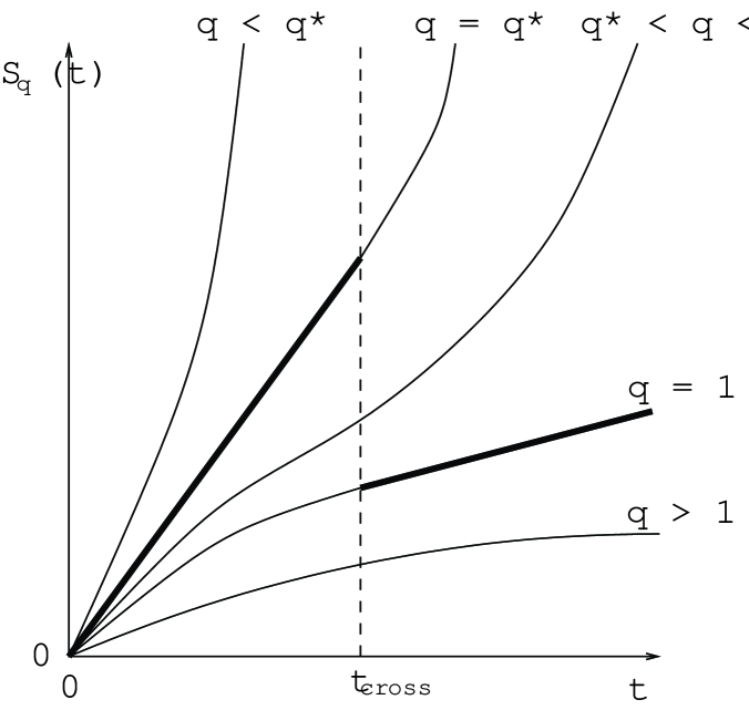
Figure 2: Schematic representation of $S_{q}(t)$ for different values of $q$, in the limit $W\to\infty$ and when there is coexistence between power-law ($q^{*}<1$) and exponential mixings. The thicker lines emphasize the linear regions.

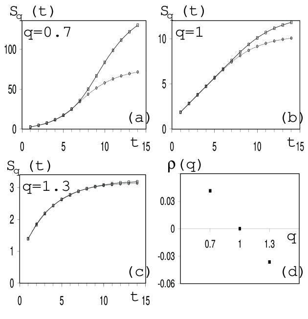
Figure 3: Typical $S_{q}(t)$ for $a=5$ (a,b,c). $1000$ histories were averaged; squares correspond to $M/10=W=708\times 708$; circles correspond to $M/10=W=224\times 224$. The lines are guides to the eye. (d) Linearity analysis $\rho(q)$ for the squares, with $t_{1}=2$ and $t_{2}=6$ (see text). The slope of $S_{1}(t)$ between $t_{1}=2$ and $t_{2}=6$ is $\widetilde{\lambda}_{1}(5)=0.96$.

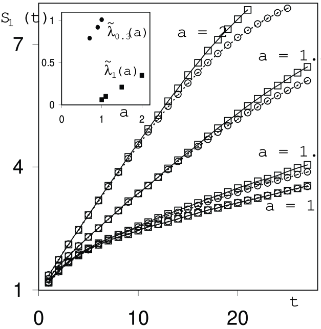
Figure 4: $S_{1}(t)$ for typical values of $a$ ($5000$ to $7000$ histories were averaged); squares correspond to $M=W=1000\times 1000$ for $a=2,1.5,1.1$ ($M=W=2236\times 2236$ for $a=1$); circles correspond to $M=W=448\times 448$ for $a=2,1.5,1.1$ ($M=W=1000\times 1000$ for $a=1$). The lines are guides to the eye. Inset: slopes of $S_{1}(t)$ and $S_{0.3}(t)$ (see also Fig. 5) in their linear stage.

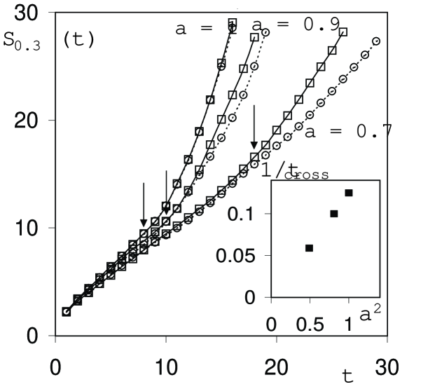
Figure 5: $S_{0.3}(t)$ for typical values of $a$ ($5000$ to $16000$ histories were averaged); squares correspond to $M=W=2236\times 2236$; circles correspond to $M=W=1000\times 1000$. The lines are guides to the eye. The arrows indicate the crossover time $t_{cross}$ for the corresponding values of $a$, as represented in the inset.

References

- [1] A. Einstein, Annalen der Physik 33, 1275 (1910) [ “Usually is put equal to the number of complexions… In order to calculate , one needs a complete (molecular-mechanical) theory of the system under consideration. Therefore it is dubious whether the Boltzmann principle has any meaning without a complete molecular-mechanical theory or some other theory which describes the elementary processes. seems without content, from a phenomenological point of view, without giving in addition such an Elementartheorie.” (Translation: Abraham Pais, Subtle is the Lord…, 1982) ]
- [2] C. Tsallis, A.R. Plastino and W.-M. Zheng, Chaos, Solitons and Fractals 8, 885 (1997). See also P. Grassberger and M. Scheunert, J. Stat. Phys. 26 697 (1981), T. Schneider, A. Politi and D. Wurtz, Z. Phys. B 66 469 (1987), G. Anania and A. Politi, Europhys. Lett. 7 119 (1988), and H. Hata, T. Horita and H. Mori, Progr. Theor. Phys. 82 897 (1989).
- [3] U.M.S. Costa, M.L. Lyra, A.R. Plastino and C. Tsallis, Phys. Rev. E 56, 245 (1997).
- [4] M.L. Lyra, C. Tsallis, Phys. Rev. Lett. 80, 53 (1998).
- [5] U. Tirnakli, C. Tsallis and M.L. Lyra, Eur. Phys. J. B 10, 309 (1999).
- [6] F.A.B.F. de Moura, U. Tirnakli and M.L. Lyra, Phys. Rev. E 62, 6361 (2000).
- [7] V. Latora, M. Baranger, A. Rapisarda, and C. Tsallis, Phys. Lett. A 273, 97 (2000); U. Tirnakli, G.F.J. Ananos and C. Tsallis, Phys. Lett. A (2001), in press [cond-mat/0005210]. See also J. Yang and P. Grigolini, Phys Lett. A 263, 323 (1999).
- [8] V. Latora, and M. Baranger, Phys.Rev. Lett. 82, 520 (1999).
- [9] C. Tsallis, J. Stat. Phys 52, 479 (1988); E.M.F. Curado, and C. Tsallis, J. Phys. A 24, L69 (1991) [Corrigenda: J. Phys. A 24, 3187 (1991), and J. Phys. A 25, 1019 (1992)]; C. Tsallis, R.S. Mendes, and A.R. Plastino, Physica A 261, 534 (1998).
- [10] C. Tsallis, in Nonextensive Statistical Mechanics and Its Applications, eds. S. Abe and Y. Okamoto, Lecture Notes in Physics 560, 3 (Springer, Berlin, 2001).
- [11] M. Tabor, Chaos and Integrability in Nonlinear Dynamics (Wiley, New York, 1989), Sec. 4.2.e.
- [12] M. Henon, in Chaotic Behavior of Deterministic Systems, eds. G. Ioos, R.H.G. Helleman, and R. Stora (North-Holland, Amsterdam, 1983).
- [13] G.M. Zaslavsky and B.A. Niyazov, Phys. Rep. 283, 73 (1997). C.
- [14] C. Tsallis, G. Bemski, and R.S. Mendes, Phys. Lett. A 257, 93 (1999).
- [15] V. Latora, A. Rapisarda and C. Tsallis, Phys. Rev. E (2001), in press (cond-mat/0103540).