Nonequilibrium and irreversible thermodynamics Solubility, segregation, and mixing; phase separation Diffusion in solids

Vacancy-mediated domain growth in a driven lattice gas.

Abstract

Using Monte Carlo simulations and a mean-field theory, we study domain growth in a driven lattice gas. Mediated by a single vacancy, two species of particles (“charges”) unmix, so that a disordered initial configuration develops charge-segregated domains which grow logarithmically slowly. An order parameter is defined and shown to satisfy dynamic scaling. Its scaling form is computed analytically, in excellent agreement with simulations.

Introduction. Driven diffusive lattice gases, first introduced by Katz, et.al. [1], display generic non-equilibrium features in their whole phase space [2]. Even when interactions are due to excluded volume constraints alone, complex phase diagrams can be induced by local dynamic rules [3, 4, 5] which violate detailed balance [6]. While disordered phases and universal properties near continuous transitions are quite well understood by now, ordered phases have proven far more complex [2]. In particular, studies of phase ordering and coarsening in driven systems have revealed surprising behaviors, quite distinct from those [7] exhibited by systems evolving towards an equilibrium final state. For example, when driven, the two-dimensional (2D) Ising lattice gas develops non-universal domain morphologies which grow in a highly anisotropic fashion and do not satisfy dynamic scaling [8]. In 1D, ordered domains grow with time as $t^{1/2}$ [9], in contrast to the equilibrium $t^{1/3}$ law [10]. Analytic results are sparse and focus primarily on establishing growth laws [9, 5, 11, 12]. Clearly, further studies of domain growth far from equilibrium are needed before a more general framework can be established.

In this letter, we report a detailed dynamic scaling analysis for defect-mediated domain growth in a driven three-state lattice gas [3]. Two species of particles, labelled “positive” and “negative”, diffuse on a periodic lattice by hopping onto a single empty site (the defect). Only nearest-neighbor jumps are allowed, biased by an “electric” field $E$ aligned with a lattice axis. At finite vacancy concentration, this system exhibits a phase transition, controlled by drive and particle density, from a disordered, “free-flowing” phase to an ordered, “jammed” phase [3, 13, 14]. Ordered configurations are spatially inhomogeneous: positive and negative particles form adjacent strips transverse to $E$, impeding each other. A mean-field theory predicts the structure and stability limits of both phases [3, 14, 15]. Models of this type have been invoked to describe water-in-oil microemulsions [16], gel electrophoresis [17] and traffic flow [18].

Remarkably, even the presence of a single vacancy suffices to order an initially random system. This problem, in both its static and dynamic aspects, is an example of a much-wider ranging class of interacting random walk and defect-mediated domain growth problems. The vacancy plays the role of a highly mobile defect [19], whose motion restructures its environment (i.e., the particle configuration), while the latter provides a feedback through the local jump rates. In the resulting steady state, investigated in detail in [20], particles form a charge-segregated strip, with the vacancy localized at one of the interfaces. The density profiles obey characteristic scaling forms, controlled by drive and system size.

Here, we focus on the time evolution of this system in 2D, seeking to understand how ordered domains form, grow and finally saturate. We present Monte Carlo (MC) data, supported by an approximate solution of the time-dependent mean-field equations. The ordering process exhibits three regimes: the initial formation of the strip, an extended logarithmic growth regime and the crossover to steady state. We demonstrate that the system satisfies dynamic scaling in the second regime and compute the scaling function analytically, in excellent agreement with the data. We conclude with some suggestions for further study. More details can be found in [21].

The microscopic model. Our model is defined on a 2D square lattice of $L_{x}\times L_{y}$ sites with fully periodic boundary conditions (PBC). The occupation of each site is represented by a spin variable $s_{xy}$ taking the values $+1,-1,0$, if a positive or negative charge or the vacancy is present at site ($x,y$). For simplicity, we restrict our study to equal densities of positive and negative charges. At each MC step (MCS), the vacancy exchanges with a randomly chosen nearest neighbor $s_{xy}$, with Metropolis rate [22], $\min\left\{1,\exp(s_{xy}E\delta y)\right\}$. Here, $\delta y=0,\pm 1$ is the change of the particle’s $y$–coordinate due to the jump. $E$ denotes the bias, uniform in space and time and directed along positive $y$.

(a)

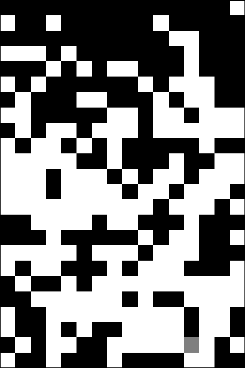
(b)

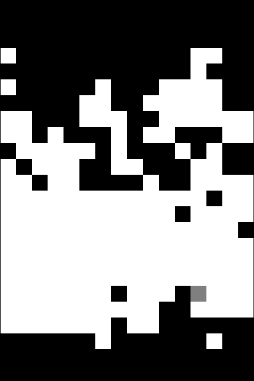
(c)

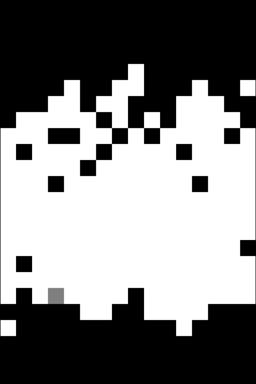
(d)

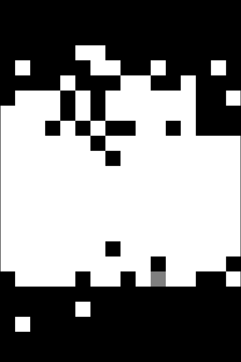
(e)

Figure 1: Snapshots of a $16\times 24$ lattice at $E=0.8$, taken after (a) $10^{3}$, (b) $10^{4}$, (c) $10^{5}$, (d) $10^{6}$, (e) $10^{7}$ MC steps. Negative (positive) particles are colored black (white), and the hole is gray. $E$ points upwards. The initial configuration was random.

This deceptively simple dynamics induces a charge segregation process on the lattice, as illustrated by Fig. 1. Starting from a random configuration (not shown), the system remains disordered for early times (Fig. 1a). Eventually, the hole begins to segregate the two species: In Fig. 1b, an interface between regions of opposite charge begins to develop. Due to PBC, a second interface must also form; this occurs at a time set by $L_{y}$. After $10^{5}$ MCS (Fig. 1c), the segregation of charges is already quite apparent. Clearly, the field drives the hole towards the lower (the “downstream”), and away from the upper (the “upstream”), interface. Typical configurations are homogeneous in the transverse direction. For our choice of parameters, the interfaces are well separated [20]. Since any increase of order requires a series of field-suppressed exchanges, the approach to steady state is very slow (Figs. 1c-e).

In the following, we provide a brief quantitative analysis of this process, beginning with our MC results. The control parameters of our study are $E$, ranging from $0.2$ to $2.0$, and the system size, $L_{x}=16$ or $40$, $16\leq L_{y}\leq 72$. The initial configuration is random. Time is measured in MCS. All of our data are averaged (denoted by $\left\langle\cdot\right\rangle$) over $100$ independent runs (samples), resulting in good statistics with errors well below $5\%$.

To probe the growth of the ordered domain, we measure averaged hole and charge density profiles, defined via $\phi(y,t){}\,\equiv\,\left\langle\frac{1}{L_{x}}\sum_{x}(1-s_{xy}^{2})\right\rangle$ and $\psi(y,t)\,\equiv\,\left\langle\frac{1}{L_{x}}\sum_{x}s_{xy}\right\rangle$. Due to translational invariance, strips can be centered at any $y$; thus, care must be taken when averaging: In each sample, we determine the maximum of the hole density over a sufficient time interval. This maximum marks the downstream interface. The charge density profiles from different samples are now shifted so that these maxima coincide, and averages can be taken. Clearly, this procedure is not very reliable for early times, since no or only faint strips have developed yet; however, our focus here concerns later stages of the growth process. Then, fluctuations of the downstream interface position are rather small and very slow, so that its location can be determined very accurately.

The evolution of the charge density profiles proceeds in three stages, as illustrated in Fig. 2 for systems with different $L_{y}$. At early times, the downstream interface forms and equilibrates quite rapidly, reaching its steady state form at about $10^{5}$ MCS, independent of $L_{y}$. Near this interface, the charges are already perfectly segregated, with the charge profile saturating at $\pm 1$. Two fronts, one on each side, separate the ordered from the remaining disordered region. The larger systems now enter a second regime, during which both fronts travel slowly outwards, increasing the width of the ordered region. This process is also independent of $L_{y}$: the centers of the fronts move out as $\ln t$, while their shape remains unchanged. Eventually, in the third regime, the two fronts merge, due to PBC, and the upstream interface equilibrates. The system has now reached steady state. For smaller systems (including the one shown in Fig. 1), the crossover to steady state sets in before well-developed fronts can form.

Figure 2: Charge density profiles for $L_{x}=16$, $E=0.8$, and a range of $L_{y}$, at different MC times (arrows). Some data points, away from the central region, are not shown for clarity.

As a quantitative probe, we define an order parameter, $\bar{Q}\equiv\sum_{y}\psi^{2}(y,t)$ [20] which measures the area, and hence the degree of order, under the (averaged, squared) charge profile. A central result of our work, Fig. 3 demonstrates that $\bar{Q}$ exhibits dynamic scaling in the logarithmic growth regime: Excellent data collapse is observed, for a range of $E$, $L_{x}$ and $L_{y}$ if $E\bar{Q}$ is plotted vs the scaling variable $\tilde{t}\equiv tE^{3}/L_{x}$. This confirms our picture of the ordering process: the motion and shape of the fronts is independent of $L_{y}$, and $\bar{Q}(\tilde{t})\propto\ln\tilde{t}$, since each escape of the vacancy is an activated process (exponentially suppressed by $E$).

Two comments are in order. First, we should emphasize that $\bar{Q}$ differs from an order parameter used previously, namely $Q\equiv\left\langle\sum_{y}\left(\frac{1}{L_{x}}\sum_{x}s_{xy}\right)^{2}\right\rangle$ [3]. The latter can be measured directly from the configurations, without the shifting procedure. Essentially, $Q$ counts the total number of ordered rows transverse to the external field. It is therefore sensitive to the presence of multiple strips which can emerge during the ordering process, especially in larger systems. As a result, the growth of $Q$ exhibits a weak $L_{y}$-dependence. In contrast, the shifting procedure averages out multiple strips, in favor of the largest (dominant) strip. Here, we focus on $\bar{Q}$ but note that the study of multiple strips remains an outstanding problem. Second, our scenario of the ordering process relies on having a well-developed downstream interface sandwiched between two fully charge-segregated regions. Our steady-state studies [20] show that this is the case provided $EL_{y}\geq 18$. Thus, the system with $L_{y}=24$, $E=0.8$ sets a lower limit.

Analytic approach. Finally, we turn to an analytic description, with the aim of deriving the appropriate scaling variables and the slope of the $\ln\tilde{t}$ law. Our starting point is a set of mean-field equations for the (coarse-grained) local hole and charge densities. Due to particle number conservation, the continuum version of our model takes the form of two continuity equations which can be derived from a microscopic master equation. Their form has been well established [3, 15, 20]. Proceeding directly to the equations for the profiles, we obtain

$$\partial_{t}\phi(y,t) = \partial\left\{\partial\phi+E\phi\psi\right\}$$ (1)

$$\partial_{t}\psi(y,t) = \partial\left\{\phi\partial\psi-\psi\partial\,\phi-E\phi\right\}$$ (2)

Here, $\partial$ denotes a spatial derivative in the drive direction, and terms of $O(\phi^{2})$ have been neglected, since they reflect the presence of multiple vacancies. The continuum limit has been taken by letting the lattice constant vanish at finite $E$. The equations have to be supplemented with appropriate boundary conditions and the constraints on total mass and charge.

Figure 3: Scaling plot of order parameter. The straight line, with slope $2.1\pm 0.1$, is a fit to the data.

Solving these coupled, nonlinear PDE’s is of course highly nontrivial. However, the data suggest a few approximations which allow for considerable analytic progress. Since we wish to capture the logarithmic growth regime, we center the downstream interface at the origin ($y=0$) and focus on the front moving in the positive $y$-direction (the other front being a mirror image, of course). By the onset of the second regime, this front is located well away from $y=0$, since the charge density at the downstream interface has already equilibrated (cf. Fig. 2). Moreover, MC data show that the hole density profile is strongly localized at the origin and does not change significantly as time progresses. Therefore, we replace it in Eq. (2) by its steady state form $\phi_{o}(y)$ [20] which decays, to excellent approximation, as $c^{-1}\exp(-E|y|)$ on both sides. Here, $c\propto L_{x}E^{-1}$ is a normalization, such that $\phi_{o}(y)$ is the probability of finding the vacancy at site ($x,y$) in the system. Introducing the scaling variables, $z\equiv Ey$ and $\tau\equiv c^{-1}E^{2}t$, we arrive [21] at a parameter-free equation, valid for $y>0$:

$$\partial_{\tau}\psi(z,\tau)=\exp(-z)\left[\partial_{z}^{2}\psi-\psi+1\right].$$ (3)

Clearly, initial and boundary conditions are needed. To study the motion of the front well before saturation occurs, we may allow $0<z<\infty$ [23]. The disordered phase far ahead of the front is modelled by $\lim_{z\rightarrow\infty}\psi(z,\tau)=0$ for all $\tau<\infty$. Further, the fully ordered phase well behind the front should be independent of $t$, since it is unaffected by further growth; thus, we demand that $\psi(z,\tau)\rightarrow 1$ for $\tau\rightarrow\infty$ and all $0<z<\infty$.

Some comments are in order. First, since $c\propto L_{x}/E$, the characteristic scaling of MC time with $E^{3}/L_{x}$ already emerges. Second, since $\bar{Q}\equiv 2\int_{0}^{\infty}\psi^{2}(y,t)dy=2E^{-1}\int_{0}^{\infty}\psi^{2}(z,\tau)dz$, our mean field theory predicts data collapse if $\bar{Q}E$ is plotted vs $tE^{3}/L_{x}$, as borne out by Fig. 3.

Since the moving front retains its shape, we may seek a solution in the form $\psi(z,\tau)\equiv f(w)$, with $w\equiv z-z_{o}(\tau)$. Clearly, $z_{o}(\tau)$ describes the front position. Eq. (3) becomes

$$-\dot{z}_{o}e^{z_{o}+w}f^{\prime}=f^{\prime\prime}-f+1,$$ (4)

where $\dot{z}_{o}\equiv$ $\partial_{\tau}z_{o}$ and $f^{\prime}\equiv\partial_{w}f$, with $\lim_{w\rightarrow+\infty}f(w)=0$ and $\lim_{w\rightarrow-\infty}f(w)=1$. Also, $f^{\prime}$ differs notably from zero only in a (finite) neighborhood of $w=0$. Multiplying both sides of (4) by $f^{\prime}$, and integrating from $-\infty$ to $+\infty$, we arrive at $\dot{z}_{o}e^{z_{o}}\int_{-\infty}^{+\infty}dwe^{w}f^{\prime 2}=\frac{1}{2}.$ Obviously, $\int_{-\infty}^{+\infty}dwe^{w}f^{\prime 2}\equiv\kappa$ is a positive, nonvanishing numerical constant. The time dependence of the front position (with simple initial condition $z_{o}(0)=0$) now follows as $z_{o}(\tau)=\ln\left(1+\tau/2\kappa\right)$. It is logarithmic, as expected.

Returning to Eq. (4), and using $\dot{z}_{o}e^{z_{o}}=1/2\kappa$, the shape of the front, subject to the specified boundary conditions, is given by $f(w)=2\kappa e^{-w}\left[1-\exp(-e^{w}/2\kappa)\right]$. The associated order parameter is now easily computed: $\bar{Q}\,E=2\ln\tau-0.927...+O(1/\tau)$, for large times $\tau>>\kappa$. Gratifyingly, the key features of the MC data, namely, the correct scaling variables, the logarithmic growth law and even its amplitude (i.e., the factor $2$) are reproduced by our solution. Of course, a single additive constant is required to match the time scale of the simulations.

Conclusions. In this letter, we presented MC and analytic results for domain growth in a simple driven lattice gas. A single vacancy rearranges positive and negative particles into charge-segregated strips transverse to the drive. Focusing on the largest strip, we find that it grows logarithmically with time, via field-suppressed excursions of the vacancy away from the center of the strip. The ordered domain is separated from the remaining disordered region by two well-defined moving fronts which retain their shape during the growth process. Eventually, the two fronts merge due to our BC’s, and the system crosses over into steady state. During the logarithmic growth regime, we observe dynamic scaling of a suitably defined order parameter, $\bar{Q}$, if $\bar{Q}E$ is plotted vs $tE^{3}/L_{x}$. These findings are supported by an (approximate) solution of a set of mean-field equations for the charge and hole density profiles. To leading order in $t$, the scaling function $\bar{Q}E$ grows as $2\ln\left(tE^{3}/L_{x}\right)$, in good agreement with the data.

Several questions remain open. First, multiple-strip configurations form easily, especially in larger systems, and our focus on the dominant strip washes out any secondary ones, due to the shifting procedure. Unfortunately, a full dynamic scaling study of observables sensitive to multiple strips demands much greater computational effort. Whether similar coarsening behavior emerges remains to be explored. A second natural extension of our study would allow for multiple vacancies, i.e., a finite hole density. Under these conditions, particles first form “clouds” which coarsen and eventually merge into multiple strips transverse to the field. These strips then continue to coarsen until a single charge-segregated strip survives. A numerical solution of the 1D mean-field equations [24] for the multiple-strip regime indicates that logarithmic growth persists, consistent with the arguments of Kafri, et.al. [11]. However, a detailed analysis, which identifies the relevant dynamic scaling variables and functions, and incorporates the crossover from clouds to strips, is still outstanding.

- [1] \NameKatz S., Lebowitz J.L. Spohn H. \REVIEWPhys. Rev. B2819831655 \REVIEWJ. Stat. Phys.341984497.
- [2] \NameSchmittmann B. Zia R.K.P. \BookPhase Transition and Critical Phenomena \Vol17 \EditorDomb C. Lebowitz J.L. \PublAcademic, New York \Year1995.
- [3] \NameSchmittmann B., Hwang K., Zia R.K.P. \REVIEWEurophys. Lett.19199219.
- [4] \NameEvans M.R., Kafri Y., Kodulevy H.M., Mukamel D. \REVIEWPhys. Rev. Lett.801998425
- [5] \NameEvans M.R., Kafri Y., Kodulevy H.M., Mukamel D. \REVIEWPhys. Rev. E5819982764. See [12] for further references to similar 1D models.
- [6] \NameMukamel D. in \BookSoft and Fragile Matter: Nonequilibrium Dynamics, Metastability and Flow \EditorCates M.E. Evans M.R. \PublInstitute of Physics Publishing, Bristol \Year2000.
- [7] \NameGunton J.D., San Miguel M., Sahni P.S. in \BookPhase Transitions and Critical Phenomena \Vol8 \EditorDomb C. Lebowitz J.L. \PublAcademic, New York \Year1983; \NameBray A.J. \REVIEWAdv. Phys.431994357.
- [8] \NameYeung C., Rogers T., Hernandez-Machado A., Jasnow D. \REVIEWJ. Stat. Phys.6619921071; \NameAlexander F.J., Laberge C.A., Lebowitz J.L., Zia R.K.P. \REVIEWJ. Stat. Phys.8219961133; \NameRutenberg A.D. Yeung C. \REVIEWPhys. Rev. E6019992710.
- [9] \NameCornell S.J. Bray A.J. \REVIEWPhys. Rev. E5419961153; \NameSpirin V., Krapivsky P.L., Redner S. \REVIEWPhys. Rev. E6019992670.
- [10] \NameCornell S.J., Kaski K., Stinchcombe R.B. \REVIEWPhys. Rev. B44199112263 \NameMajumdar S.N., Huse D.A., Lubachevsky B.D. \REVIEWPhys. Rev. Lett.731994182.
- [11] \NameKafri Y., Biron D., Evans M.R., Mukamel D. \REVIEWEur. Phys. J. B162000669 .
- [12] \NameEvans M.R., Kafri Y., Levine E., Mukamel D. \REVIEWPhys. Rev. E6220007619.
- [13] \NameBassler K.E., Schmittmann B. Zia R.K.P. \REVIEWEurophys. Lett. 241993115.
- [14] \NameLeung K.-t. Zia R.K.P. \REVIEWPhys. Rev. E561997308.
- [15] \NameVilfan I., Zia R.K.P., Schmittmann B. \REVIEWPhys. Rev. Lett.7319942071.
- [16] \NameAertsens M. Naudts J. \REVIEWJ. Stat. Phys.621990609.
- [17] \NameRubinstein M. \REVIEWPhys. Rev. Lett.5919871946; \NameDuke T.A.J. \REVIEWPhys. Rev. Lett.6219892877); \NameShnidman Y. in \BookMathematical and Industrial Problems IV \EditorFriedman A. \PublSpringer, Berlin \Year1991; \NameWidom B., Viovy J.L., Desfontaines A.D. \REVIEWJ. Phys. I (France)119911759.
- [18] \NameBiham O., Middleton A.A., Levine D. \REVIEWPhys. Rev. A461992R6124; \NameLeung K.-t. \REVIEWPhys. Rev. Lett.7319942386; \NameMolera J.M., Martinez F.C. Cuesta J.A. \REVIEWPhys. Rev. E511995175; \NameChowdhury D., Santen L., Schadschneider A. \REVIEWPhys. Rep.3292000199.
- [19] \NameToroczkai Z., Korniss G., Schmittmann B., Zia R.K.P. \REVIEWEurophys. Lett.401997281; \NameTriampo W., Aspelmeier T., Schmittmann B. \REVIEWPhys. Rev. E6120002386; \NameAspelmeier T., Schmittmann B., Zia R.K.P. \REVIEWPhys. Rev. Lett.87200165701.
- [20] \NameThies M. Schmittmann B. \REVIEWPhys. Rev. E612000184.
- [21] \NameSchmittmann B. Thies M. to be published.
- [22] \NameMetropolis N., Rosenbluth A.W., Rosenbluth M.N., Teller A.H. Teller E. \REVIEWJ. Chem. Phys.2119531087.
- [23] These boundary conditions are already implicit in the normalization of .
- [24] \NameKertész J. Ramaswamy R. \REVIEWEurophys.Lett.281994617.