Applications and Sexual Version of

a Simple Model for Biological Ageing

A. O. SOUSA¹, S. MOSS DE OLIVEIRA¹ and D.STAUFFER²

¹Instituto de Física, Universidade Federal Fluminense, Av. Litorânea s/n, Boa Viagem, 24210-340 Niterói, RJ, Brasil.

²Inst. for Theor. Physics, Cologne University, D-50923 Köln, Euroland.

e-mail: sousa@if.uff.br, suzana@if.uff.br, stauffer@thp.uni-koeln.de

Abstract We use a simple model for biological ageing to study the mortality of the population, obtaining a good agreement with the Gompertz law. We also simulate the same model on a square lattice, considering different strategies of parental care. The results are in agreement with those obtained earlier with the more complicated Penna model for biological ageing. Finally, we present the sexual version of this simple model.

Keywords: population dynamics, ageing, Monte Carlo simulations, Evolution

1 Introduction

One theory for biological ageing is the accumulation of bad inherited mutations. While the well known Penna model [1] uses a genome represented by a bitstring, this simple model [2] reduces the genetic information, transmitted with mutations from one generation to the next, to two integers, the minimum reproduction age $a_{m}$ and the genetic death age $a_{d}$. At each iteration, every individual with age $a$ between $a_{m}$ and $a_{d}$ gets at most one child (birth rate $b=1$) which inherits these numbers, apart from random changes (mutations) by $\pm 1$. Individuals die with certainty if their age reaches $a_{d}$, and they die earlier with probability $N(t)/N_{max}$ at every iteration, where $N(t)$ is the actual population and $N_{max}$ a so-called carrying capacity taking into account the limitations of food and space (Verhulst factor). The probability $p_{b}(i)$ for individual $i$ to get a child takes into account the well known (see e.g. [3]) trade-off between fecundity and survival and is the lower the larger the difference $a_{d}-a_{m}$ is:

$$p_{b}(i)=(1+0.08)/(a_{d}(i)-a_{m}(i)+0.08)$$

where the constant 0.08 ensures that the denominator is never zero. (For the mutations we require $0\leq a_{m}<a_{d}\leq 32$ to facilitate comparison with the Penna model which typically has 32 age intervals.)

This simple model allows for a self-organization (“emergence”) of a broad distribution of $a_{m}$ values, and a relatively more narrow distribution of $a_{d}$ values [2] (similar but not identical to those shown below in Fig.6; the $a_{m}$ distribution gets more narrow relatively if, as in section 4, an increase of $a_{m}$ is coupled to an increase of $a_{d}$.). It explained the catastrophic senescence of Pacific Salmon [4], the vanishing of cod in the northwest Atlantic through overfishing [5], and allowed to take into account the social needs of humans for a minimum population size [5]. But only with a birth rate increasing in old age [6] could a reasonable agreement with the Gompertz law be achieved.

Figure 1: Mortality function $\mu$ versus age (in iterations) giving rough agreement with the Gompertz law; $\beta=0.7$ with and without Verhulst deaths using 9 million individuals.

In the next section we present the mortality obtained with a slightly modified version of this model, which then agrees with the Gompertz law. In section 3 we present the results of the model when the individuals are placed on a square lattice and live under some parental care strategies. Finally, in section 4 we present the sexual version of the model and conclusions.

2 The Gompertz law

To get the Gompertz law of an exponentially increasing mortality function of age $a$, we now follow [7] and assume the genetic deaths to be probabilistic instead of deterministic, with probability $p_{d}=1/\{1+\exp[\beta(a_{d}-a)]\}$ and $\beta=0.7$; the deterministic case is recovered for $\beta\rightarrow\infty$. The survival probability thus decays like a Fermi function in physics. Fig.1 shows a good agreement with the exponential increase of the mortality function [9, 8] $\mu(a)=\ln[S(a-1/2)/S(a+1/2)]$ for humans at middle age (where $S(a)$ is the number of survivors at age $a$; $\mu$ approximates the derivative $-d(\ln S)/da$). For the deterministic case, $\beta\rightarrow\infty$, the analogous plot is strongly curved. Alternatively one may omit [10] the condition that no age exceeds 32, increase the constant from 0.08 to about 2, and set $\beta=0.3$; then Fig.2 shows a similar increase of the mortality function with age, with a reasonable distribution of genetic death ages which is no longer cut off at 32.

Figure 2: As Fig.1 but $\beta=0.3$ with 609 million individuals including Verhulst deaths, no maximum age and 0.08 replaced by 2.0 in the birth rate.

3 Parental care on a square lattice

Figure 3: Final distribution of the population on the lattice considering that if the mother moves, she brings the children under maternal care (age $\leq 2$) with her (case a). The final distribution of the lattice considering that the mother cannot move, if she has children under maternal (case b), looks very similar (not shown).

Now we return to the original deterministic version of the model and place the individuals on a square lattice. The carrying capacity $N_{max}$ is now replaced by a maximum occupation per site $N_{max}(i,j)$, such that the new Verhulst probability for an individual to die due to environmental restrictions depends on the current number of individuals $N_{(i,j)}(t)$ on each site. We give to each individual a probability $p_{m}$ to move to the neighbouring site that presents the smallest occupation, if this occupation is also smaller or equal to that of the current individual’s site. The strategy of child-care consists in defining a maternal care period $A_{pc}$ during which no child can move. We considered the following conditions: (a) if the mother moves, she brings the young children with her; (b) the mother cannot move if she has any child still under maternal care. In Fig. 3 we show the lattice configurations after 800,000 steps for case (a). The result of case (b) is very similar and not shown. These same strategies were simulated before using the Penna model [11], giving these same results. Also following [11], we simulated a third case which corresponds to case (a) with the restriction that if the mother dies, her children still under maternal care have a further probability to die. Figure 4 shows the spatial configuration for this case (c). Again the result is the same obtained with the Penna model, despite of the simplicity of the present model. Fig.5 compares the population sizes of the three cases. The parameters used to produce figures 3, 4 and 5 are: initial population = 10,000 individuals; maximum occupation per site = 30 individuals; initial minimum reproduction age $a_{m}=1$; initial genetic death age $a_{d}=16$; birth rate $b=2$; maternal care period $A_{pc}=2$ and lattice size = $150\times 150$.

Figure 4: Final distribution of the lattice considering that if the mother moves she brings the children under maternal care with her, and that if she dies, her children have a probability $0.9$ to die in their first year of life, and $0.3$ in their second year of life (case c). In this case we used a maximum occupation per site equal to 42 individuals. Even so, the final configuration of the lattice is much smaller than those obtained in cases (a) and (b).

Figure 5: Number of individuals as a function of time for cases: a (circles), b (triangles) and c (squares).

4 The sexual version

Now the population consists of males and females. At each iteration, every female with age $a$ between $a_{m}$ and $a_{d}$ randomly chooses a male, also with age between $a_{m}$ and $a_{d}$, to mate. The child randomly inherits the $a_{m}$ and $a_{d}$ values from one of the parents, independently. Mutations are introduced in the following way: two random numbers are generated; if they are both positive, $a_{m}$ and $a_{d}$ are both increased by one. If they are both negative, $a_{m}$ and $a_{d}$ are decreased by one; if the signs of the random numbers are different, no mutation occurs. Notice that in this way the difference $a_{m}-a_{d}$ is maintained constant. This strategy simulates the fact that a recessive mutation, to be effective, must be inherited from both parents; alternatively, it can be interpreted as antagonistic pleiotropy, the trade-off between fecundity and longevity [8, 3]. One may also regard this sexual version as an alternative to the requirement of a minimal population for human society [5]: a single individual cannot reproduce. In Fig. 6 we show the histograms of $a_{m}$ and $a_{d}$, that is, the number of individuals with a given value of $a_{d}$ and the number of individuals with a given value of $a_{m}$. It can be seen that there is also, as in the asexual case [2], a self-organization of distributions of $a_{m}$ and $a_{d}$. We have also tried to introduce the mutations in $a_{m}$ and $a_{d}$ independently of each other: Then no self-organization appears, that is, the $a_{m}$ value goes always to 1 and the $a_{d}$ value, to 32.

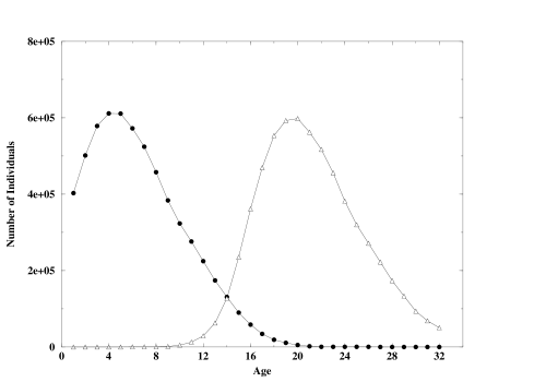
Figure 6: Distribution of minimum age of reproduction (circles) and of genetic death age (triangles) after a stationary state has been reached for the sexual population. Parameters: initial population = 25,000 males plus 25,000 females; maximum population size $N_{max}=500,000$, initial $a_{m}=1$ and initial $a_{d}=16$.

As in many previous simulations, starting with Redfield [12, 13], the sexual version does not give a clear advantage over the asexual one and additional assumptions like in [14] may be needed to justify sex.

5 Conclusion

The simple alternative [2] to the more widespread Penna model [1, 8] of biological ageing via inherited mutations was modified here to give reasonable agreement with the Gompertz mortality law at middle and old age, to allow a more realistic description of spatial fluctuations on a lattice, and to include sexual reproduction. In all cases the results were similar to those obtained earlier in the Penna model. Further research could concentrate on the simplification [10], to omit the restriction $a_{d}\leq 32$ and to omit the parameter now taken as 0.08.

Acknowledgements: A. O. Sousa and S. Moss de Oliveira thank CAPES, CNPq and FAPERJ for financial support; DS thanks the Jülich Supercomputer Center for time on their Cray-T3E.

References

- [1] T.J.P. Penna, J. Stat. Phys. 78, 1629 (1995)
- [2] D. Stauffer, in Biological Evolution and Statistical Physics (Dresden, May 2000), edited by M. Lässig and A. Valleriani, Springer, Berlin-Heidelberg 2002
- [3] C.K. Galambor, T.E. Martin, Science 292, 494 (2001)
- [4] H. Meyer-Ortmanns, Int. J. Mod. Phys. C 12, 319 (2001)
- [5] D. Stauffer and J.P. Radomski, preprint
- [6] D. Makowiec, D. Stauffer and M. Zieliński, Int. J. Mod. Phys. C 12, No. 7 (2001)
- [7] J. Thoms, P. Donahue, N. Jan, J. Physique I 5, 935 (1995)
- [8] S. Moss de Oliveira, P.M.C. de Oliveira, D. Stauffer: Evolution, Money, War and Computers, Teubner, Stuttgart and Leipzig 1999
- [9] L.D. Mueller, T.J. Nusbaum and M.R. Rose, Exp. Gerontol. 30, 553 (1995)
- [10] P.M.C. de Oliveira, priv. comm., June 2001
- [11] A.O. Sousa and S. Moss de Oliveira, Eur. Phys. J. B 9, 365 (1999)
- [12] R.J. Redfield, Nature 369, 145 (1994); similarly S. Siller, Nature 411, 689 (2001)
- [13] D. Stauffer, P.M.C. de Oliveira, S. Moss de Oliveira, T.J.P. Penna, J.S. Sá Martins, An. Acad. Bras. Ci. 73, 15 (2001)
- [14] J.S. Sá Martins and D. Stauffer, Physica A, 294, 191 (2001)