Theory of coherent Bragg spectroscopy of a trapped Bose-Einstein condensate

Abstract

We present a detailed theoretical analysis of Bragg spectroscopy from a Bose-Einstein condensate at $T=0$K. We demonstrate that within the linear response regime, both a quantum field theory treatment and a meanfield Gross-Pitaevskii treatment lead to the same value for the mean evolution of the quasiparticle operators. The observable for Bragg spectroscopy experiments, which is the spectral response function of the momentum transferred to the condensate, can therefore be calculated in a meanfield formalism. We analyse the behaviour of this observable by carrying out numerical simulations in axially symmetric three-dimensional cases and in two dimensions. An approximate analytic expression for the observable is obtained and provides a means for identifying the relative importance of three broadening and shift mechanisms (meanfield, Doppler, and finite pulse duration) in different regimes. We show that the suppression of scattering at small values of $q$ observed by Stamper-Kurn et al., [Phys. Rev. Lett. 83, 2876 (1999)] is accounted for by the meanfield treatment, and can be interpreted in terms of the interference of the $u$ and $v$ quasiparticle amplitudes. We also show that, contrary to the assumptions of previous analyses, there is no regime for trapped condensates for which the spectral response function and the dynamic structure factor are equivalent. Our numerical calculations can also be performed outside the linear response regime, and show that at large laser intensities a significant decrease in the shift of the spectral response function can occur due to depletion of the initial condensate.

I Introduction

In 1999 Ketterle’s group at MIT reported a set of experiments in which condensate properties were measured using the technique of Bragg spectroscopy Stenger et al. (1999); Stamper-Kurn et al. (1999). In those experiments a low intensity Bragg pulse was used to excite a small amount of condensate into a higher momentum state, and the Bragg spectrum of the condensate was found by measuring the momentum transfer for a range of Bragg frequencies ($\omega$) and momenta ($\hbar\mathbf{q}$). That work established Bragg spectroscopy as a tool capable of measuring condensate properties with spectroscopic precision. The theoretical analysis of the measurements however, gives rise to a number of issues. Ketterle and his colleagues assumed that the spectra gave a direct measurement of the dynamic structure factor, which is the Fourier transform of the density-density correlation function, and is familiar as the observable in neutron scattering experiments in super-fluid heliumPines and Nozieres (1966,1990,1999, 1990,1999); Griffin (1993). They also attributed the suppression of imparted momentum they observed at low $q$ values to correlated pair excitations, and quantum depletion of the condensate, and speculated Stamper-Kurn and Ketterle (2001) that an accurate description would require a more complete quantum treatment. The purpose of the current paper is to develop a theory of Bragg spectroscopy that is valid in the regime of the experiments, and to use it to make quantitative calculations and to analyze the phenomena that occur in this regime. We also investigate the relationship between the observable of Bragg spectroscopy (i.e. the momentum transferred to the condensate) and the dynamic structure factor, and show that for a trapped condensate there is no regime in which one can simply be obtained from the other.

We begin in section II within the framework of many body field theory and calculate, in the Bogoliubov approximation, the linear response of the condensate to an applied Bragg pulse. We obtain expressions for the temporal evolution of the quasiparticle operators, and show that they have a nonzero mean value, i.e. that the quasiparticles are generated as coherent states. We demonstrate that within a well defined regime the mean values of the Bogoliubov operators are identical to the amplitudes obtained from a linearized mean-field (Gross-Pitaevskii) treatment. The meanfield treatment therefore provides a valid description of the experiments in the regime of small excitation.

A number of meanfield theoretical treatments of Bragg scattering from condensates have been given. Blakie and Ballagh have presented a quantitative meanfield description Blakie and Ballagh (2000) which confirmed the analysis of the Bragg spectroscopy shift given by the MIT group, and provided analytic estimates for a number of quantities, including the momentum width of the scattered condensate. Stringari and colleagues have also used a meanfield description to analyze Bragg spectroscopy Zambelli et al. (2000); Brunello et al. (2001), and in addition have used the approach to devise schemes for measuring quasiparticle amplitudes Brunello et al. (2000), and for making spatially separate condensates interfere Pitaevskii and Stringari (1999). In the current paper we use the Gross Pitaevskii formulation of Bragg scattering as presented by Blakie and Ballagh Blakie and Ballagh (2000) to analyze the behavior observed in the Bragg spectroscopy experiments.

The observable in the experiments is the momentum transferred to the condensate, and in section III we define a normalized version of the expectation value of this quantity that we call the spectral response function $R(\mathbf{q},\omega)$. For a trapped condensate the momentum transfer can arise from two sources, the Bragg beams or the trap itself, which complicates the analysis. The MIT group recognized this issue, and applied the Bragg laser pulses only for a small fraction of the trap period, and then released the trap. However the tradeoff involved in minimizing momentum transfer from the trap by using a short Bragg pulse significantly compromises the energy selectivity of the process. We examine the influence this has on the relationship between $R(\mathbf{q},\omega)$ and the dynamic structure factor $S(\mathbf{q},\omega)$, and we show that in the presence of a trap, the evaluation of $S(\mathbf{q},\omega)$ requires $R(\mathbf{q},\omega)$ to be known for all possible pulse lengths.

The central quantity of Bragg spectroscopy is thus the spectral response function $R(\mathbf{q},\omega)$ and we derive an approximate analytic expression for this quantity, incorporating the effects of both the meanfield interaction and the finite duration of the Bragg pulse, in section IV. In section V we use $R(\mathbf{q},\omega)$ to characterize our numerical investigations of Bragg spectroscopy, and we consider a wide range of three dimensional axially symmetric scenarios, for which we simulate the experiments using the meanfield (Gross Pitaevskii) equation for Bragg scattering Blakie and Ballagh (2000). We verify the validity range of our approximate form for $R(\mathbf{q},\omega)$ by comparing it to the full numerical results, and we identify the regimes in which one or other of the mechanisms of: the meanfield interaction, the Doppler effect, and the finite pulse duration, dominates the formation of the Bragg spectrum. We also show that our approximate form for $R(\mathbf{q},\omega)$ will allow a more accurate estimation of the momentum width of a condensate than obtained by previous analyses.

Our numerical simulations allow us to calculate the effect on Bragg spectroscopy of laser intensities sufficiently large that linear response theory no longer holds. We investigate cases where the scattered fraction of the condensate is of order 20%, and show that the depletion of the ground state condensate leads to a significant reduction of the frequency shift, which has not been accounted for in previous analyses. We also consider the spectral response function from a vortex, using two dimensional simulations. Finally in section VI we investigate the energy response of a condensate subject to a Bragg pulse of sufficiently long duration that individual quasiparticle excitations can be resolved.

II Low-intensity Bragg scattering theory

In this section we calculate the response of the condensate to a Bragg pulse within the linear regime, using two distinct approaches. In the first of these (section IIA) we use the many body field theory formalism in the Bogoliubov approximation, to calculate the temporal evolution of the quasiparticle operators. In the second approach (section IIB) we use a meanfield (Gross Pitaevskii) equation and obtain the amplitudes of the linearized response. The two approaches are shown to give identical mean results in section IIC.

II.1 Many-body field theoretic approach

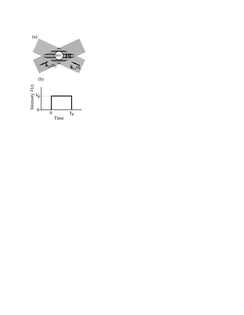
Figure 1: Bragg spectroscopy of a Bose-Einstein condensate (BEC). (a) Two laser beams with wavevectors $\mathbf{k}_{1}$ and $\mathbf{k}_{2}$ and frequencies $\omega_{1}$ and $\omega_{2}$ respectively, create a moving optical potential with wavevector $\mathbf{q}=\mathbf{k}_{1}-\mathbf{k}_{2}$ and frequency $\omega=\omega_{1}-\omega_{2}$ (see Blakie and Ballagh (2000)). (b) Temporal behaviour of the Bragg pulse assumed in this paper.

The many-body Hamiltonian for $N_{0}$ identical bosons in a trap and subject to a time-dependent Bragg pulse can be written

$$\hat{H}=\hat{H}_{0}+\hat{H}_{I}(t),$$ (1)

where $\hat{H}_{0}$ is the usual trapped boson Hamiltonian

$$\hat{H}_{0}=\int d\mathbf{r}\,\hat{\Psi}^{\dagger}\left[-\frac{\hbar^{2}}{2m}\nabla^{2}+V_{T}(\mathbf{r})\right]\hat{\Psi}+\frac{U_{0}}{2}\int d\mathbf{r}\,\hat{\Psi}^{\dagger}\hat{\Psi}^{\dagger}\hat{\Psi}\hat{\Psi}.$$ (2)

$V_{T}(\mathbf{r})$ is the trapping potential, which we choose to be harmonic. The Bragg interaction $\hat{H}_{I}(t)$ arises from two overlapping plane wave laser fields, which have equal amplitudes but frequency and wave vector differences $\omega$ and $\mathbf{q}$ respectively (see Fig. 1(a)). The laser fields are treated classically, and their interaction with the internal transition of the atoms is characterized by a Rabi frequency $\Omega(t)$ (for the combined fields at the intensity peaks) and a detuning $\Delta$ which is large and essentially the same for both laser fields. In this regime the internal structure for the atoms can be eliminated (see Blakie and Ballagh (2000) for details) so that the field operator $\hat{\Psi}$ refers only to the ground internal state, and $\hat{H}_{I}(t)$ takes the form

$$\hat{H}_{I}(t)=\int d\mathbf{r}\,\hat{\Psi}^{\dagger}\left[\hbar V(t)\cos(\mathbf{q}\cdot\mathbf{r}-\omega t)\right]\hat{\Psi},$$ (3)

where $V(t)=\Omega^{2}(t)/2|\Delta|$ (see Fig. 1(a)).

II.1.1 Bogoliubov transformation

For a highly occupied stationary state ($T\approx 0$K) the field operator can be written in the Bogoliubov approximation as a sum of meanfield and operator parts ($\hat{\Psi}=\langle\hat{\Psi}\rangle+\hat{\phi}$). In this paper we mostly consider a ground state, but we also consider the case of a central vortex. Following standard treatments (e.g. Griffin (1996); Fetter (1972)) we employ a Bogoliubov transformation for the operator part to write

$$\hat{\Psi}(\mathbf{r},t) = \sqrt{N_{0}}\psi_{0}(\mathbf{r})e^{-i\mu t}+e^{i(S_{0}(\mathbf{r})-\mu t)}\times$$

$$\sum_{i}\left(\hat{b}_{i}(t)e^{-i\omega_{i}t}\tilde{u}_{i}(\mathbf{r})+\hat{b}^{\dagger}_{i}(t)e^{i\omega_{i}t}\tilde{v}^{*}_{i}(\mathbf{r})\right),$$

where the condensate is represented by the first term, and $\hat{b}_{i}$ and $\hat{b}^{\dagger}_{i}$ are the quasiparticle destruction and creation operators respectively (in an interaction picture with respect to $\hat{H}_{0}$). The state $\psi_{0}=|\psi_{0}|\exp(iS_{0})$, is an eigenstate solution, with eigenvalue $\hbar\mu$ of the time independent Gross-Pitaevskii equation

$$\hbar\mu\psi_{0}=\left[-\frac{\hbar^{2}}{2m}\nabla^{2}+V_{T}(\mathbf{r})\right]\psi_{0}+N_{0}U_{0}|\psi_{0}|^{2}\psi_{0},$$ (5)

and the functions $\{\tilde{u}_{i},\tilde{v}_{i}\}$ are the orthogonal quasiparticle basis states Morgan et al. (1998). These basis states are orthogonal to the condensate mode and are related to the usual (non-orthogonal) quasiparticle basis states $\{u_{i},v_{i}\}$ (given below) by projection into the subspace orthogonal to the condensate, i.e.

$$\tilde{u}_{i} = u_{i}-a_{i}|\psi_{0}|,$$ (6)

$$\tilde{v}_{i}^{*} = v_{i}^{*}+a^{*}_{i}|\psi_{0}|,$$ (7)

where

$$a_{i}=\int d\mathbf{r}\,|\psi_{0}|u_{i}=-\int d\mathbf{r}\,|\psi_{0}|v_{i},$$ (8)

(see Morgan et al. (1998)).

The form of Bogoliubov transformation used in Eq. (II.1.1) explicitly includes the phase ($S_{0}$) of $\psi_{0}$, which is convenient in cases where $\psi_{0}$ is not necessarily a ground state. We note that a number of different sign conventions appear in the literature, and ours differs from that in Ref. Fetter (1972). We discuss the different conventions in the Appendix. The Bogoliubov-de Gennes equation for $\{u_{i},v_{i}\}$ are

$${\cal L}u_{i}+N_{0}U_{0}|\psi_{0}|^{2}v_{i} = \hbar\omega_{i}u_{i},$$ (9)

$${\cal L}^{*}v_{i}+N_{0}U_{0}|\psi_{0}|^{2}u_{i} = -\hbar\omega_{i}v_{i},$$ (10)

where

$${\cal L}=\left[-{\hbar^{2}\over 2m}(\nabla+i\nabla S_{0})^{2}+V_{T}(\mathbf{r})-\hbar\mu+2N_{0}U_{0}|\psi_{0}|^{2}\right],$$ (11)

with the orthogonality conditions

$$\int d\mathbf{r}\{u_{i}u_{j}^{*}-v_{i}v_{j}^{*}\} = \delta_{ij},$$ (12)

$$\int d\mathbf{r}\{u_{i}v_{j}-v_{i}u_{j}\} = 0.$$ (13)

II.1.2 Bogoliubov Hamiltonian

Applying the transformation in Eq. (II.1.1), to the Hamiltonians (2) and (3) we obtain their Bogoliubov form, i.e.

$$\hat{H}_{0} \approx \hat{H}_{0}^{B}$$ (14)

$$\equiv E_{0}+\sum_{i}\hbar\omega_{i}\hat{b}_{i}^{\dagger}\hat{b}_{i},$$

$$\hat{H}_{I}(t) \approx \hat{H}^{B}_{I}(t)$$

$$\equiv N_{0}\int d\mathbf{r}\,|\psi_{0}|^{2}\hbar V(t)\cos(\mathbf{q}\cdot\mathbf{r}-\omega t)$$

$$+\sqrt{N_{0}}\sum_{i}\Big{[}\hat{b}_{i}^{\dagger}e^{i\omega_{i}t}\int d\mathbf{r}\,(\tilde{u}_{i}^{*}+\tilde{v}_{i}^{*})$$

$$\times\hbar V(t)\cos(\mathbf{q}\cdot\mathbf{r}-\omega t)|\psi_{0}|+\rm{h.c}\Big{]},$$

where $E_{0}$ is the energy of the highly occupied state (see Eq. (76)). The quasiparticle transformation diagonalizes $\hat{H}_{0}$ to quadratic order, and we note that the orthogonal basis $\{\tilde{u}_{i},\tilde{v}_{i}\}$ is required for this diagonalization to be valid. In evaluating $\hat{H}^{B}_{I}$, terms involving products of quasiparticle operators have been ignored. This amounts to neglecting Bragg induced scattering between quasiparticle states, which is of order $1/\sqrt{N_{0}}$ smaller than the terms linear in $\hat{b}_{i}^{\dagger}$ (or $\hat{b}_{i}$). Those linear terms are of primary interest here, as they describe the scattering between the condensate and quasiparticle states which occurs as a result of the energy and momentum transfer from the optical potential.

The time dependent exponentials, $\exp(\pm i\omega_{i}t)$, which multiply the quasiparticle operators in Eq. (II.1.1) account for the free evolution due to $\hat{H}^{B}_{0}$, and so the Heisenberg equation

$$i\hbar\frac{\partial}{\partial t}\left(\hat{b}_{i}e^{-i\omega_{i}t}\right)=\left[\left(\hat{b}_{i}e^{-i\omega_{i}t}\right),\hat{H}_{0}^{B}+\hat{H}^{B}_{I}(t)\right],$$ (16)

becomes

$$i\hbar\frac{\partial}{\partial t}\hat{b}_{i} = \left[\hat{b}_{i},\hat{H}_{0}^{B}+\hat{H}^{B}_{I}(t)\right]-\hbar\omega_{i}\hat{b}_{i},$$ (17)

$$= \left[\hat{b}_{i},\hat{H}_{I}^{B}(t)\right].$$ (18)

This is easily solved to give

$$\hat{b}_{i}(t)=\hat{b}_{i}(0)-\beta_{i}(t),$$ (19)

where $\beta_{i}(t)$ is a $c$-number,

$$\beta_{i}(t) = -i\sqrt{N_{0}}\int_{0}^{t}dt^{\prime}\,V(t^{\prime})e^{i\omega_{i}t^{\prime}}\int d\mathbf{r}\,$$ (21)

$$\times(\tilde{u}^{*}_{i}+\tilde{v}^{*}_{i})\cos(\mathbf{q}\cdot\mathbf{r}-\omega t^{{}^{\prime}})|\psi_{0}|.$$

We see that the Bragg excitation causes the quasiparticle operators to develop nonzero mean values. Note that this is a complete solution of the physics in the linearized regime, from which any observable quantities can be computed.

II.1.3 Initial conditions

Our derivation so far has been based on a $T=0$K Bogoliubov treatment. For this case the initial state is the quasiparticle vacuum state ($|0\rangle$). Had we started with this initial condition and considered evolution in the Schrödinger picture we would have found that the system evolves as $|0\rangle\rightarrow\exp(i\theta)|\{\beta_{i}\}\rangle$, where $|\{\beta_{i}\}\rangle$ is a coherent state, i.e. $\hat{b}_{i}|\{\beta_{i}\}\rangle=\beta_{i}|\{\beta_{i}\}\rangle$ and $\theta$ is some phase factor (see Gardiner and Zoller (1999)).

Equation (19) also provides insight into finite temperature cases where most of the atoms are in the condensate. To fully treat the finite temperature case, it is necessary to generalize the Bogoliubov treatment to account for the thermal depletion (e.g. see Griffin (1996)), requiring the functions $\psi_{0}$, $u_{i}$, $v_{i}$ and $\omega_{i}$ to be solved for in a self-consistent manner (e.g. see Hutchinson et al. (1997, 1998); Morgan (2000)). In that case, Eq. (19) for the evolution of $\hat{b}_{i}$ will still apply, and thus we see that the initial statistics of $\hat{b}_{i}(0)$ are preserved and the mean value $\langle\hat{b}_{i}\rangle$ is shifted by $\beta_{i}$.

II.2 Gross-Pitaevskii equation approach

The Gross-Pitaevskii equation for a condensate of $N_{0}$ particles subject to a Bragg pulse was derived in Blakie and Ballagh (2000), i.e.

$$i\hbar{\partial\over\partial t}\Psi(\mathbf{r},t) = \left[-{\hbar^{2}\over 2m}\nabla^{2}+V_{T}(\mathbf{r})+U_{0}|\Psi|^{2}\right]\Psi(\mathbf{r},t)$$ (22)

$$+\hbar V(t)\cos(\mathbf{q}\cdot\mathbf{r}-\omega t)\Psi(\mathbf{r},t),$$

where $\Psi(\mathbf{r},t)$ is the condensate meanfield wavefunction for the atoms in their internal ground state, and is normalized according to $\int d\mathbf{r}\,|\Psi|^{2}=N_{0}$. The condensate wavefunction can be expanded in terms of a quasiparticle basis in the form

$$\Psi(\mathbf{r},t) = \sqrt{N_{0}}\psi_{0}e^{-i\mu t}+e^{i(S_{0}(\mathbf{r})-\mu t)}$$

$$\times\sum_{i}\left(c_{i}(t)u_{i}e^{-i\omega_{i}t}+c^{*}_{i}(t)v_{i}^{*}e^{i\omega_{i}t}\right),$$

where $c_{i}$ are the time dependent quasiparticle amplitudes. This expansion has been made using the non-orthogonal quasiparticle basis, and the ground state has been assumed static. This latter assumption will only be valid while excitation induced by the Bragg pulse remains small. The wavefunction decomposition (Eq. (II.2)) transforms the Gross-Pitaevskii Eq. (22) into

$$i\hbar \sum_{i}\left(\dot{c}_{i}(t)u_{i}e^{-i\omega_{i}t}+\dot{c}^{*}_{i}(t)v_{i}^{*}e^{i\omega_{i}t}\right)$$ (25)

$$=e^{-i(S_{0}(\mathbf{r})-\mu t)}\hbar V(t)\cos(\mathbf{q}\cdot\mathbf{r}-\omega t)\Psi(\mathbf{r},t).$$

Morgan et al. Morgan et al. (1998) have shown how to use the orthogonality relations of the quasiparticles, Eqs. (12) and (13), to project out the quasiparticle amplitudes from a condensate wavefunction, namely

$$c_{j}(t) = e^{i\omega_{j}t}\int d\mathbf{r}\,\left[e^{i(\mu t-S_{0}(\mathbf{r}))}u_{j}^{*}\Psi-v_{j}^{*}e^{-i(\mu t-S_{0}(\mathbf{r}))}\Psi^{*}\right]$$ (26)

$$-2a_{j}^{*},$$

where $a_{j}$ is defined in Eq. (8). Since the quasiparticles form a complete set, we may use projection to obtain a set of equations for quasiparticle amplitudes that are equivalent to Eq. (25), namely

$$\dot{c}_{j}(t) = -iV(t)e^{i\omega_{i}t}\int d\mathbf{r}\,\Big{[}u_{j}^{*}e^{i(\mu t-S_{0}(\mathbf{r}))}\cos(\mathbf{q}\cdot\mathbf{r}-\omega t)\Psi$$ (27)

$$+v_{j}^{*}e^{-i(\mu t-S_{0}(\mathbf{r}))}\cos(\mathbf{q}\cdot\mathbf{r}-\omega t)\Psi^{*}\Big{]}.$$

Because the quasiparticles occupations are all small compared to the condensate mode, we can simplify Eq. (27) by setting $\Psi(\mathbf{r},t)=\sqrt{N_{0}}|\psi_{0}(\mathbf{r})|\exp(iS_{0}(\mathbf{r})-i\mu t)$, yielding

$$c_{i}(t) = -i\sqrt{N_{0}}\int_{0}^{t}dt^{\prime}\,V(t^{\prime})e^{i\omega_{i}t^{\prime}}\int d\mathbf{r}\,(u^{*}_{i}+v^{*}_{i})$$ (28)

$$\times\cos(\mathbf{q}\cdot\mathbf{r}-\omega t^{{}^{\prime}})|\psi_{0}|.$$

This will of course only provide a good solution while the quasiparticle occupations all remain small.

II.3 Comparison of approaches

Direct comparison of the Gross-Pitaevskii and quantum field theoretic results is complicated by the fact that they have been derived for different basis sets. We note that although the Gross-Pitaevskii analysis was carried out using the $\{u_{i},v_{i}\}$ basis, it is equally straightforward to use the orthogonal basis $\{\tilde{u}_{i},\tilde{v}_{i}\}$. Morgan et al. Morgan et al. (1998) have shown that (in analysis of the Gross-Pitaevskii equation) transforming between these bases affects only the ground state population and gives rise to no difference in the quasiparticle occupations.

Connections between the field theory and simple Gross-Pitaevskii results based on Eq. (22) can only be expected to exist at $T=0$K, where thermal effects can be ignored . In this regime we begin by considering the relevant vacuum expectation of the quasiparticle operator from Eq. (19)

$$\langle\hat{b}_{i}(t)\rangle = -i\sqrt{N_{0}}\int_{0}^{t}dt^{\prime}\,V(t^{\prime})e^{i\omega_{i}t^{\prime}}\int d\mathbf{r}\,(\tilde{u}^{*}_{i}+\tilde{v}^{*}_{i})$$ (29)

$$\times\cos(\mathbf{q}\cdot\mathbf{r}-\omega t^{\prime})|\psi_{0}|.$$

This expression emphasizes the coherent nature of the quasiparticle states, and is the same as the Gross-Pitaevskii result of Eq. (28), with the identification $c_{i}(t)\leftrightarrow\langle\hat{b}_{i}(t)\rangle$. We note that the apparent difference between equations (28) and (29), where the former depends on the matrix elements involving $\{u_{i},v_{i}\}$ and the latter on matrix elements involving $\{\tilde{u}_{i},\tilde{v}_{i}\}$, disappears with the observation that $u_{i}+v_{i}=\tilde{u}_{i}+\tilde{v}_{i}$ (see Eqs. (6) and (7)). Thus we have verified that the $c_{i}(t)$ and $\langle\hat{b}_{i}(t)\rangle$ are identical.

II.4 Quasiparticle occupation

For the physics we consider in this paper the mean occupation of the $i$-th quasiparticle level (i.e. $\langle\hat{b}^{\dagger}_{i}\hat{b}_{i}\rangle$ or $|c_{i}(t)|^{2}$ for the many-body or Gross-Pitaevskii methods respectively) is of interest, as it is used to make a quasi-homogeneous approximation to the spectral response function in Eq. (59). Using Eq. (19) we calculate

$$\langle\hat{n}_{i}(t)\rangle = N_{0}\Big{|}\int_{0}^{t}dt^{\prime}\,e^{i\omega_{i}t^{\prime}}V(t^{\prime})\int d\mathbf{r}\,(u_{i}^{*}+v_{i}^{*})$$ (30)

$$\times\cos(\mathbf{q}\cdot\mathbf{r}-\omega t^{\prime})|\psi_{0}|\Big{|}^{2}+\langle\hat{n}_{i}(0)\rangle,$$

where $\langle\hat{n}_{i}(0)\rangle$ is the initial occupation, e.g. thermal occupation at $T\neq 0$K , and is included for generality. In Eq. (30) we have chosen to use the $\{u_{i},v_{i}\}$ quasiparticle basis for ease of comparison with previous results by other authors (e.g. Csordás et al. (1996); Fetter and Rokhsar (1998); Zambelli et al. (2000); Wu and Griffin (1996)).

To progress, it is necessary to specify the temporal behavior of the Bragg pulse. For simplicity we take the pulse shape as being square, with $V=V_{p}$ for $0<t<T_{p}$ (see Fig. 1(b)), then Eq. (29) becomes (evaluated at $t=T_{p}$)

$$\langle\hat{b}_{i}(T_{p})\rangle = -i\sqrt{N_{0}}V_{p}e^{i(\omega_{i}-\omega)T_{p}/2}\Big{[}\left(\frac{\sin((\omega_{i}-\omega)T_{p}/2)}{(\omega_{i}-\omega)}\right)\int d\mathbf{r}\,(u_{i}^{*}+v_{i}^{*})e^{i\mathbf{q}\cdot\mathbf{r}}|\psi_{0}|$$ (31)

$$+e^{i\omega T_{p}}\left(\frac{\sin((\omega_{i}+\omega)T_{p}/2)}{(\omega_{i}+\omega)}\right)\int d\mathbf{r}\,(u_{i}^{*}+v_{i}^{*})e^{-i\mathbf{q}\cdot\mathbf{r}}|\psi_{0}|\Big{]}.$$

In this expression, the second term (with denominator $\omega_{i}+\omega$) will typically be significantly smaller than the first term (with denominator $\omega_{i}-\omega$) since $\omega>0$, so to a good approximation we can ignore the second term. Similarly, the quasiparticle occupation result (30) under the same approximation is

$$\langle\hat{n}_{i}(T_{p})\rangle = \frac{\pi V_{p}^{2}T_{p}N_{0}}{2}\left|\int d\mathbf{r}\,(u_{i}^{*}+v_{i}^{*})e^{i\mathbf{q}\cdot\mathbf{r}}|\psi_{0}|\right|^{2}$$ (32)

$$\times F(\omega_{i}-\omega,T_{p})+\langle\hat{n}_{i}(0)\rangle,$$

in which

$$F(\omega,T)=\frac{2\sin^{2}(\omega T/2)}{\pi T\,\omega^{2}},$$ (33)

is a familiar term in time dependent perturbation calculations. In particular $F(\omega_{i}-\omega,T_{p})$ in Eq. (32) is sharply peaked in frequency about $\omega=\omega_{i}$, encloses unit area and has a half width of $\sigma_{\omega}\sim 2\pi/T_{p}$. In the limit $T_{p}\to\infty$ (while $V_{p}^{2}T_{p}$ remains small) this term can be taken as a $\delta$-function expressing precise energy conservation, so that only quasiparticles of energy $\hbar\omega$ will be excited, i.e.

$$\lim_{T_{p}\to\infty}\langle\hat{n}_{i}(T_{p})\rangle = \frac{\pi V_{p}^{2}T_{p}N_{0}}{2}\left|\int d\mathbf{r}(u^{*}_{i}+v^{*}_{i})e^{i\mathbf{q}\cdot\mathbf{r}}|\psi_{0}|\right|^{2}$$ (34)

$$\times\delta(\omega-\omega_{i})+\langle\hat{n}_{i}(0)\rangle.$$

III Observable of Bragg spectroscopy

In this section we outline the experimental procedure of Bragg spectroscopy on condensates. We begin by discussing the measured observable, which we refer to as the spectral response function. In Stenger et al. (1999); Stamper-Kurn et al. (1999) this observable was assumed to be a measurement of the dynamic structure factor. We briefly review the dynamic structure factor, and discuss why it is inappropriate for these experiments.

III.1 Spectral response function

In the MIT experiments Stamper-Kurn et al. (1999); Stenger et al. (1999) a low intensity Bragg grating was used to excite the condensate in-situ for less than a quarter of a trap period. Immediately following this the trap was turned off, the system allowed to ballistically expand, and the momentum transfer to the system was inferred by imaging the expanded spatial distribution. The experimental signal measured is (see Stenger et al. (1999); Stamper-Kurn et al. (1999); Stamper-Kurn and Ketterle (2001))

$$R(\mathbf{q},\omega)=\gamma\,\frac{P(T_{p})-P(0)}{\hbar q},$$ (35)

where

$$\gamma^{-1}={\pi\over 2}N_{0}V_{p}^{2}T_{p},$$ (36)

and $P$ is the momentum expectation of the system. We shall refer to $R(\mathbf{q},\omega)$ as the spectral response function. For the case of a Gross-Pitaevskii wavefunction, the spectral response function can be written as

$$R(\mathbf{q},\omega)=\gamma\,\frac{\int d\mathbf{r}\,\Psi^{*}(\mathbf{r},T_{p})\left(-i{\hbar\nabla}\right)\Psi(\mathbf{r},T_{p})}{\hbar q},$$ (37)

where it is assumed that the initial condensate has zero momentum expectation value. The factors $\gamma$ and $\hbar q$ appearing in Eqs. (35) and (37) effectively scale out effects of the Bragg intensity and duration, the magnitude of momentum transfer, and condensate occupation, so that $R(\mathbf{q},\omega)$ can be interpreted as a rate of excitation per atom (normalized with respect to $V_{p}^{2}$) within the condensate.

III.2 Dynamic structure factor

The dynamic structure factor has played an important role in the analysis of inelastic neutron scattering in superfluid ⁴He. It has facilitated the understanding of collective modes, and has enabled measurements of the pair distribution function and condensate fraction in that system, as discussed extensively in Griffin (1993). In those experiments a monochromatic neutron beam of momentum $\hbar\mathbf{k}_{0}$ is directed onto a sample of ⁴He and the intensity of neutrons scattered to momentum $\hbar\mathbf{k}^{{}^{\prime}}$ is measured. van Hove van Hove (1954) showed that the inelastic scattering cross section of thermal neutrons, calculated in the first Born approximation, can be directly expressed in terms of the quantity

$$S(\mathbf{q},\omega) = \frac{1}{\mathcal{Z}}\sum_{m,n}e^{-\beta E_{m}}|\langle m|\hat{\rho}_{\mathbf{q}}|n\rangle|^{2}\delta(\hbar\omega-E_{m}+E_{n}),$$

which is called the dynamic structure factor (see Pines and Nozieres (1966,1990,1999)). In Eq. (III.2), $|m\rangle$ and $E_{m}$ are the eigenstates and energy levels of the unperturbed system, $\mathcal{Z}$ is the partition function, $\hat{\rho}_{\mathbf{q}}=\int d\mathbf{r}\,\hat{\Psi}^{\dagger}(\mathbf{r})\exp(-i\mathbf{q}\cdot\mathbf{r})\hat{\Psi}(\mathbf{r})$ is the density fluctuation operator, and we have taken

$$\hbar\omega = \frac{\hbar^{2}k_{0}^{2}}{2m}-\frac{\hbar^{2}k^{\prime 2}}{2m},$$ (39)

$$\mathbf{q} = \mathbf{k}_{0}-\mathbf{k}^{{}^{\prime}}.$$ (40)

Our choice of notation for these quantities is to facilitate comparison between the matrix elements which arise in the dynamic structure factor and Bragg cases. We note that in the Bragg context $\mathbf{q}$ and $\omega$ refer to the wave vector and frequency respectively of the optical potential, whereas in a dynamic structure factor measurement, $\hbar\mathbf{q}$ and $\hbar\omega$ are the momentum and energy respectively, transferred to the system from the scattered probe.

For the case of a trapped gas Bose condensate, low intensity off resonant inelastic light scattering Javanainen (1995) provides a close analogy to neutron scattering from ⁴He. Csordás et al. Csordás et al. (1996) have shown that the cross section for such inelastic light scattering, with energy and momentum transfer to the photon of $-\hbar\omega$ and $-\hbar\mathbf{q}$ respectively, can be expressed in terms of the quantity

$$S(\mathbf{q},\omega) = \sum_{i}\left|\int d\mathbf{r}\,(u_{i}^{*}+v_{i}^{*})e^{i\mathbf{q}\cdot\mathbf{r}}|\psi_{0}|\right|^{2}$$

$$\times\left((\langle\hat{n}_{i}\rangle+1)\delta(\omega-\omega_{i})+\langle\hat{n}_{i}\rangle\delta(\omega+\omega_{i})\right).$$

This expression generalizes the dynamic structure factor to the case of light scattering and applies at finite temperatures in the regime of linear response, where the Bogoliubov theory for quasiparticles is valid. At $T=0$K, where thermal depletion can be ignored, the dynamic structure factor (III.2) takes the form

$$S_{0}(\mathbf{q},\omega) = \sum_{i}\left|\int d\mathbf{r}(u^{*}_{i}+v^{*}_{i})e^{i\mathbf{q}\cdot\mathbf{r}}|\psi_{0}|\right|^{2}\delta(\omega-\omega_{i}),$$ (42)

$$\qquad\qquad\qquad\qquad(T=0\rm{K})$$

for which a number of approximate forms have been calculated (e.g. see Csordás et al. (1996); Wu and Griffin (1996); Zambelli et al. (2000)).

The dynamic structure factor and Bragg spectroscopy

Although the dynamic structure factor and the spectral response function are distinctly different quantities, they do resemble each other strongly. In fact, the matrix elements in the $T=0$K dynamic structure factor in (42) resemble those in the expression (34) for the Bragg induced quasiparticle population, $\langle\hat{n}_{i}\rangle$ in the long time limit. It is easy to show, beginning from (42), that

$$S_{0}(\mathbf{q},\omega)=\left\{\gamma{\sum_{i}}\lim_{T_{p}\to\infty}\langle\hat{n}_{i}(T_{p})\rangle\right\},\qquad(T=0\rm{K})$$ (43)

where $\langle\hat{n}_{i}\rangle$ is given by Eq. (34) and $\gamma$ is defined in Eq. (36). Note that because Eq. (43) is evaluated at $T=0$K, we have taken the initial occupation, $\langle\hat{n}_{i}(0)\rangle$ in Eq. (34), to be zero. In practice a very long pulse ($T_{p}\gg 1/\omega_{T}$) of sufficiently weak intensity ($V^{2}_{p}T_{p}\ll 1$) could be used to excite the quasiparticles in the regime necessary for Eq. (43) to hold.

In Stamper-Kurn et al. (1999); Stenger et al. (1999) the spectral response function $R(\mathbf{q},\omega)$ was assumed to represent a measurement of the dynamic structure factor, $S(\mathbf{q},\omega).$ The argument given in those papers was based on the assumption that the Bragg pulse would excite quasiparticles of definite momentum $\hbar\mathbf{q}$ and the momentum transfer is hence proportional to the rate of quasiparticle excitation. This is in fact not so, although we can show that, in a certain sense, the dynamic structure factor and the spectral response function do determine each other. We use the result of Brunello et al. Brunello et al. (2001), who have shown that the momentum imparted can be related to the dynamic structure factor according to

$$\frac{dP_{z}(t)}{dt}=-m\omega_{z}^{2}Z+2N_{0}\hbar q\left(\frac{V}{2}\right)^{2}\int d\omega^{\prime}\,\left[S(\mathbf{q},\omega^{\prime})-S(-\mathbf{q},-\omega^{\prime})\right]\frac{\sin([\omega-\omega^{\prime}]t)}{\omega-\omega^{\prime}},$$ (44)

where the Bragg scattering has been taken to be in the $z$-direction and $P_{z}$ is the $z$-component of the momentum expectation. The quantity $Z=\langle\sum^{N}_{j=1}z_{j}\rangle$ is the expectation value of the $z$ center of mass coordinate and evolves according to

$$\frac{dZ}{dt}=\frac{P_{z}}{m}.$$ (45)

Taking the initial position and momentum expectations to be zero, Eqs. (44) and (45) can be solved using (35) to give the spectral response function in terms of the dynamic structure factor as

$$R(\mathbf{q},\omega)=\frac{1}{\pi T_{p}}\int d\omega^{\prime}\left[S(\mathbf{q},\omega^{\prime})-S(-\mathbf{q},-\omega^{\prime})\right]\frac{\cos(\omega_{z}T_{p})-\cos([\omega-\omega^{\prime}]T_{p})}{[\omega-\omega^{\prime}]^{2}-\omega_{z}^{2}}.$$ (46)

This formula can be inverted, but the inversion formulae are different depending on whether $\omega_{z}$ is zero or not:

$$S(\mathbf{q},\omega)-S(-\mathbf{q},-\omega) = \lim_{T_{p}\to\infty}R(\mathbf{q},\omega,T_{p})\qquad\qquad\quad\mbox{for $\omega_{z}=0$},$$ (47)

$$= \omega_{z}^{2}\int_{0}^{\infty}R({\bf q},\omega,T_{p})\,T_{p}dT_{p}\qquad\qquad\quad\mbox{for $\omega_{z}\neq 0$}.$$ (48)

In the linearized approximation we are using, we can use (III.2) to show that

$$S_{0}(\mathbf{q},\omega) = S(\mathbf{q},\omega)-S(-\mathbf{q},-\omega),\qquad\omega\geq 0,$$ (49)

so that the differencing cancels out finite temperature effects. Beyond the Bogoliubov approximation, there will however be residual finite-temperature effects.

Thus we see it is possible to determine the zero temperature dynamic structure factor in a good degree of approximation from experiments on a trapped condensate, provided measurements are performed for a sufficient range of pulse times $T_{p}$. It is clear that this could be a difficult experiment to implement, since the spectral response function will drop off faster than $1/T_{p}$ for large $T_{p}$, so the measured signal could become very small. But in analogy with the results of Sect.VI, we would expect that significant information could be obtained by measuring for pulse times $T_{p}$ up to about 5 trap periods.

On the other hand there is no direct connection between the spectral response function and the dynamic structure factor for any single time $T_{p}$ unless $\omega_{z}=0$, in which case we must take $T_{p}\to\infty$. In fact, if we note that significant structure in $S({\bf q},\omega)$ is expected on the frequency scale of $\omega_{z}$, then the formula (46) shows that a smearing over this frequency scale is assured by the form of the integrand in (46), independently of the value of $T_{p}$.

One therefore must conclude that the spectral response function, not the dynamic structure factor, is the appropriate method of analysis for Bragg scattering experiments. However, it is in principle possible to determine the zero temperature dynamic structure factor in a certain degree of approximation from these experiments by use of the inversion formula (48).

IV Quasi-homogeneous approximation to $R(\mathbf{q},\omega)$

In this section we develop an approximation for the spectral response function valid for time scales shorter than a quarter trap period. Because trap effects are negligible on this time scale we employ a quasi-homogeneous approach, based on homogeneous quasiparticles weighted by the condensate density distribution. This approximation plays an important part in the analysis of the numerical results we present in section V.

IV.1 Homogeneous spectral response

The results developed in section II for the trapped condensates can be applied to a homogeneous system of number density $n$ by making the replacements

$$u_{i}(\mathbf{r}) \rightarrow u_{k}(n)e^{i\mathbf{k}\cdot\mathbf{r}}/\sqrt{\mathcal{V}},$$ (50)

$$v^{*}_{i}(\mathbf{r}) \rightarrow v_{k}(n)e^{-i\mathbf{k}\cdot\mathbf{r}}/\sqrt{\mathcal{V}},$$ (51)

$$\sqrt{N_{0}}\psi_{0}(\mathbf{r}) \rightarrow \sqrt{N_{0}/\mathcal{V}}=\sqrt{n,}$$ (52)

where $\mathcal{V}$ is the volume, and

$$u_{k}(n) = \frac{\omega^{B}_{k}(n)+\omega_{k}}{2\sqrt{\omega^{B}_{k}(n)\omega_{k}}}\,,$$ (53)

$$v_{k}(n) = -\frac{\omega^{B}_{k}(n)-\omega_{k}}{2\sqrt{\omega^{B}_{k}(n)\omega_{k}}}\,,$$ (54)

$$\omega^{B}_{k}(n) = \sqrt{\omega^{2}_{k}+2nU_{0}\omega_{k}/\hbar}\,,$$ (55)

$$\omega_{k} = \frac{\hbar k^{2}}{2m}\,.$$ (56)

We have explicitly written these as functions of density $n$ for later convenience. Using Eqs. (50)-(52) the expectation of the quasiparticle operators (31) (i.e. at $T=0$K) resulting from Bragg excitation is found to be

$$\langle\hat{b}_{\mathbf{k}}\rangle = -iV_{p}\sqrt{\frac{n}{\mathcal{V}}}\int_{\mathcal{V}}d\mathbf{r}\,(u_{k}(n)e^{-i\mathbf{k}\cdot\mathbf{r}}+v_{k}(n)e^{-i\mathbf{k}\cdot\mathbf{r}})e^{i\omega^{B}_{k}(n)T_{p}/2}\Big{[}e^{-i\omega T_{p}/2}\left(\frac{\sin((\omega^{B}_{k}(n)-\omega)T_{p}/2)}{(\omega^{B}_{k}(n)-\omega)}\right)e^{i\mathbf{q}\cdot\mathbf{r}}$$ (57)

$$\quad+\,e^{i\omega T_{p}/2}\left(\frac{\sin((\omega^{B}_{k}+\omega)T_{p}/2)}{(\omega^{B}_{k}+\omega)}\right)e^{-i\mathbf{q}\cdot\mathbf{r}}\Big{]}.$$

Since the homogeneous excitations are plane waves, evaluating the spatial integral in Eq. (57) selects out quasiparticles with wave vector $\mathbf{k}=\pm\mathbf{q}$. The occupations $\langle\hat{b}_{\mathbf{k}}^{\dagger}\hat{b}_{\mathbf{k}}\rangle$ of these states are

$$\langle\hat{n}_{\pm\mathbf{q}}\rangle=\frac{\pi V_{p}^{2}T_{p}N_{0}}{2}(u_{q}(n)+v_{q}(n))^{2}F((\omega^{B}_{q}(n)\mp\omega),T_{p}),$$ (58)

where $F(\omega,T)$ is defined in Eq. (33). Since a quasiparticle created by $\hat{b}_{\mathbf{k}}^{\dagger}$ carries momentum $\hbar\mathbf{k}$, the total momentum transferred to the homogeneous condensate is

$$\langle\mathbf{p}\rangle\ =\hbar\mathbf{q}\left(\langle\hat{n}_{\mathbf{q}}\rangle-\langle\hat{n}_{-\mathbf{q}}\rangle\right),$$ (59)

and the spectral response function, as defined in Eq. (35), becomes

$$R(\mathbf{q},\omega)=\gamma\,\frac{\left|\langle\mathbf{p}\rangle\right|}{\hbar q},$$ (60)

$$\,=\gamma\,\left(\langle\hat{n}_{\mathbf{q}}\rangle-\langle\hat{n}_{-\mathbf{q}}\rangle\right),$$ (61)

$$\,=\frac{\omega_{q}}{\omega^{B}_{q}(n)}\Big{[}F((\omega^{B}_{q}(n)-\omega),T_{p})-F((\omega^{B}_{q}(n)+\omega),T_{p})\Big{]},$$

(62)

where we have used $(u_{q}(n)+v_{q}(n))^{2}=\omega_{q}/\omega^{B}_{q}(n)$ (from Eqs. (53) and (54)) to arrive at the last result.

IV.2 Quasi-homogeneous spectral response function

The density distribution of a Thomas-Fermi condensate is given by

$$N(n)=\frac{15N_{0}}{4n^{2}_{p}}n\sqrt{1-n/n_{p}},$$ (63)

where $N(n)dn$ is the portion of condensate atoms in the density range $n\rightarrow n+dn$, and $n_{p}=\hbar\mu/U_{0}$, is the peak density (see Stenger et al. (1999)).

To approximate the spectral response function for the inhomogeneous case we multiply the portion of the condensate at density $n$ by the homogeneous spectral response function (62) for a homogeneous condensate (of density $n$) and integrate over all densities present, i.e.

$$R_{QH}(\mathbf{q},\omega) \equiv \int dn\,N(n)R(\mathbf{q},\omega),$$

$$= \left(\frac{15N_{0}}{4n^{2}_{p}}\right)\int^{n_{p}}_{0}dn\,\frac{n\,\omega_{q}}{\omega^{B}_{q}(n)}\sqrt{1-n/n_{p}}$$

$$\times\Big{[}F(\omega^{B}_{q}(n)-\omega,T_{p})-F(\omega^{B}_{q}(n)+\omega,T_{p})\Big{]}.$$

We shall refer to $R_{QH}$ as the finite time quasi-homogeneous approximation to the spectral response function, or simply the quasi-homogeneous approximation. Ignoring the finite time broadening effects and assuming exact energy conservation in $R_{QH}$ with the replacement $F(\omega,T)\rightarrow\delta(\omega)$, reduces Eq. (IV.2) to the simpler line-shape expression

$$R_{QH}(\mathbf{q},\omega) \rightarrow I_{q}(\omega),$$ (66)

$$= \frac{15\hbar(\omega^{2}-\omega^{2}_{q})}{8\omega_{q}N_{0}U_{0}}\sqrt{1\!-\!\frac{\hbar(\omega^{2}-\omega^{2}_{q})}{2\omega_{q}N_{0}U_{0}}},$$ (67)

where we have adopted the notation, $I_{q}$, as used in the original derivation Stenger et al. (1999). Equation (67) is also known as the local density approximation to the dynamic structure factor (see Zambelli et al. (2000)), and has been used to analyze experimental data in Stenger et al. (1999); Stamper-Kurn et al. (1999). We emphasize that with $T_{p}<(1/4)\,T_{\rm{trap}}$ the $\delta$-function replacement is unjustifiable, as we verify with our numerical results in the next section.

V Bragg spectroscopy

Bragg spectroscopy can broadly be defined as selective excitation of momentum components in a condensate, by Bragg light fields. In this section we consider the spectral response function as a Bragg spectroscopic measurement, and using numerical simulations of the Gross-Pitaevskii equation (22) and the analytic results of the previous section we identify the dominant physical mechanisms governing the spectral response behavior. We investigate the spectral response function for a vortex and identify parameter regimes in which a clear signature of a vortex is apparent. From the full numerical simulations we are also able to assess the effect of higher laser intensities on the spectroscopic measurements.

V.1 Numerical results for $R(\mathbf{q},\omega)$

V.1.1 Procedure

The numerical results we present for $R(\mathbf{q},\omega)$, are found by evolving an initial stationary condensate state (typically a ground state) in the presence of the Bragg optical potential, using Eq. (22). At the conclusion of this pulse, the spectral response is evaluated using Eq. (37). This differs slightly from the typical procedure in the experiments, where the system is allowed to expand before destructive imaging is used to measure the condensate momentum. However we have verified numerically (in cylindrically symmetric 3D cases) that condensate expansion (after the pulse) does not alter the momentum expectation value. For each desired value of $\mathbf{q}$ and $\omega$, we repeat our procedure of evolving $\Psi$ according to (22), and calculating $R(\mathbf{q},\omega)$ immediately after the optical pulse terminates.

For axially symmetric situations, the simulations are calculated in three spatial dimensions with $\mathbf{q}$ oriented along the $z$-axis. When the initial state is a vortex, the interesting case of scattering in a direction orthogonal to the vortex core (lying on the $z$-axis) would break the symmetry requirement, so for these cases 2D simulations with $\mathbf{q}$ directed along the $y$-axis are used. For convenience we use computational units of distance $r_{0}=\sqrt{\hbar/2m\omega_{T}}$; interaction strength $w_{0}=\hbar\omega_{T}r_{0}^{3}$; and time $t_{0}=\omega_{T}^{-1}$ ; where $\omega_{T}$ is the trapping frequency in the direction of scattering.

V.1.2 Parameter regimes

We use square pulses of intensity and duration such that typically less than $1\%$ of the condensate is excited, except in section V.5 where we investigate the nonlinear response of the condensate. As long as the amount of excitation is small, we verify that the spectral response function $R({\bf q},\omega)$ is independent of $V_{p}$. However, the shape of $R({\bf q},\omega)$ is dependent on the pulse duration (in accordance with the frequency spread about $\omega$ associated with the time limited pulse) and on the magnitude of $\mathbf{q}$.

The momentum $\hbar q_{0}$ defined by

$$\hbar q_{0}=\sqrt{2mn_{p}U_{0}},$$ (68)

(i.e. $q_{0}=1/\xi$, where $\xi$ is the condensate healing length) characterizes the division between regimes of phonon and free particle-like quasiparticle character. We note that the experimental results in Stenger et al. (1999) and Stamper-Kurn et al. (1999) report measurements of $R(\mathbf{q},\omega)$ in the free particle and phonon regime, respectively.

V.2 Underlying broadening mechanisms

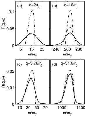
Figure 2: Spectral response function $R(\mathbf{q},\omega)$ of a 3D condensate. (a), (b) Spherical condensate, $N_{0}U_{0}=10^{4}w_{0}$, $\mu=14.2\omega_{T}$. (c), (d) Oblate condensate with trap asymmetry $\lambda=\sqrt{8}$, $N_{0}U_{0}=5.6\times 10^{5}w_{0}$, $\mu=70.9\omega_{T}$. Full numerical solution for $R$ shown as solid line; the local density approximation ($I_{q}$) dash-dot; and the finite time local density approximation ($R_{QH}$) dashed. Bragg parameters are $V_{p}=0.2\omega_{T}$ and $T_{p}=0.4/\omega_{T}.$

We present in Fig. 2 spectral response functions calculated using the Gross-Pitaevskii simulations in three spatial dimensions. The spectral response functions in Figs. 2(a) and (b) are for a spherically symmetric ground state with $q_{0}=3.8/r_{0}.$ The $q$ values (of the Bragg fields) were chosen so that the case in Fig. 2(a) is in the phonon regime ($q=2/r_{0}$), while Fig. 2(b) is in the free particle limit ($q=16/r_{0}$). For comparison, we present in Figs. 2(c) and (d) spectral response functions for a different ground state of greater nonlinearity, for which $q_{0}=8.4/r_{0}$. Fig. 2(c) is in the phonon regime ($q=3.76/r_{0}$), whereas Fig. 2(d) is in the free particle regime ($q=31.6/r_{0}$). In all cases we compare the Gross-Pitaevskii calculation of $R$ with the lines-shape $I_{q}$ and quasi-homogeneous result $R_{QH}$ from Eqs. (67) and (IV.2) respectively.

V.2.1 Mechanisms

The two ground states used in calculating the results presented in Fig. 2 are both in the Thomas-Fermi limit (i.e. they satisfy the condition $\mu\gg\omega_{T}$). We can see from the figure that the local density approximation $I_{q}$ Eq. (67) used by previous authors does not always give a good description of $R(\mathbf{q},\omega)$, whereas our quasi-homogeneous approximation $R_{QH}(\mathbf{q},\omega)$ Eq. (IV.2) is much more accurate. We have investigated the accuracy of $R_{QH}$ over a wide parameter range which has allowed us to evaluate the relative importance of the three underlying broadening mechanisms which contribute to $R(\mathbf{q},\omega)$. The mechanisms and their contributions are as follows:

• The shift in the excitation spectrum due to the meanfield interaction (depending on the local density). The range of densities present in the condensate cause a spread in this shift. The frequency width associated with this spread is proportional to the chemical potential $\mu$, and we shall refer to this as the density width - see section IV.

• The Doppler effect due to the momentum spread of the condensate; the Doppler broadened frequency width is $\sigma_{p}\cdot q/m$, where $\sigma_{p}$ is the condensate momentum width.

• The frequency spread in the Bragg grating due to the finite pulse time; the width arising from this effect is $\sim\pi/T_{p}$.

V.2.2 Relative importance of mechanisms

The relative importance of these mechanisms varies according to the parameter regime. In Table 1 we compare the estimated values of these widths for the simulations in Fig. 2.

	density	finite $T_{p}$	momentum
Fig.	$\mu$	$\pi/T_{p}$	$\sigma_{p}\cdot q/m$
2(a)	14.2	7.9	0.86
2(b)	14.2	7.9	6.92
2(c)	70.6	7.9	0.88
2(d)	70.6	7.9	7.4

Table 1: Simple estimate of widths of component mechanisms of the spectral response functions in Fig. 2. All quantities expressed in units of $\omega_{T}$.

We see that for the case of Fig. 2(a) both finite time and density effects are important; hence the quasi-homogeneous result which includes both of these is in good agreement with $R(\mathbf{q},\omega)$, whereas $I_{q}(\omega)$ which accounts for density effect alone is quite inaccurate. In Fig. 2(b) the value of $q$ is much larger, increasing the momentum width to a point where it is comparable to the other mechanisms. Since both $I_{q}$ and $R_{QH}$ fail to account for the condensate momentum, neither approximation to the spectral response function is in particularly good agreement with the numerically calculated $R$. In both Figs. 2(c) and (d) the density width is an order of magnitude larger than both the finite pulse and momentum widths, and so in this regime the simple line-shape expression $I_{q}$ is generally adequate.

V.2.3 Experimental comparison

Taking typical experimental parameters, the state used in Figs. 2(a) and (b) corresponds to about $2.8\times 10^{5}$ Na atoms in a $50$ Hz trap, with the Bragg grating formed from $589$ nm laser beams intersecting at an angle of $5^{\circ}$ in (a) and $39^{\circ}$ in (b). These figures are indicative of typical Bragg spectroscopy results for a small to medium size condensate. The state used in Figs. 2(c) and (d) corresponds to about $10^{7}$ Na atoms in a $100$ Hz trap, and was chosen to match some of the features of the experiments reported in Stenger et al. (1999); Stamper-Kurn et al. (1999), e.g. the peak density of this state is $\sim 4\times 10^{14}$ atoms/cm³ and the chemical potential is $\sim 6.7$kHz. The momentum values chosen correspond to those used to probe the phonon and free particle regimes in those papers (Bragg grating formed by $589$ nm beams at $14^{\circ}$ and $180^{\circ}$ respectively). Computational constraints mean we cannot match the experimental (prolate) trap geometry, but in a similar manner to the measurements made in Stenger et al. (1999) we scatter along a tightly trapped direction, although from a condensate in an oblate trap of aspect ratio $\sqrt{8}$. We note that in the phonon probing experiments Stamper-Kurn et al. (1999), scattering was performed in the weakly trapped direction for imaging convenience. It is worth emphasizing that the mechanisms accounted for in our approximate response function $R_{QH}$ depend only on the peak density (i.e. $\hbar\mu/U_{0}$), the magnitude of $q$ and the Bragg pulse duration. The reason is that condensates in the Thomas-Fermi regime with the same peak density will have identical density distributions in either prolate or oblate traps (see Eq. (63)). Thus the quasi-homogeneous approximation predicts the same spectral response function for both. Scattering in a tightly trapped direction will enhance momentum effects not accounted for in $R_{QH}$, since spatially squeezing the condensate causes the corresponding momentum distribution to broaden. However, it is apparent from Table 1, that for the case of large condensates this momentum effect is relatively small, and thus we expect our result in Figs. 2(c) and (d) to give a reasonably accurate description of the MIT experiments Stenger et al. (1999); Stamper-Kurn et al. (1999).

V.3 Spectral response function of a vortex

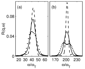
Figure 3: Spectral response functions $R(\mathbf{q},\omega)$ for 2D ground (solid) and $m=1$ vortex (dots) states, and $R_{QH(2D)}$ for 2D ground state (dashed). Both states have $N_{0}U_{0}=500w_{0}$, and the spectra are calculated with (a) $q=6/r_{0}$ and (b) $q=14/r_{0}$. Bragg parameters are $V_{p}=0.2\omega_{T}$ and $T_{p}=0.8/\omega_{T}$.

In previous work Blakie and R. J. Ballagh (2001) we showed how Bragg scattering from a vortex can produce an asymmetric spatially selective beam of scattered atoms which provides an in-situ signature of a vortex. In Fig. 3 we compare the spectral response functions from two dimensional ground and vortex states, and in Table 2 we summarize the density, finite time and momentum effects for the cases in Fig. 3.

	density	finite time	momentum
Fig.	$\mu$	$\pi/T_{p}$	$\sigma_{p}\cdot q/m$
3(a) ground	9.0	3.9	2.9
3(a) vortex	9.2	3.9	5.2
3(b) ground	9.0	3.9	6.7
3(b) vortex	9.2	3.9	12.2

Table 2: Simple estimate of widths of component mechanisms of the spectral response functions in Fig. 3. All quantities expressed in units of $\omega_{T}$.

In the low momentum transfer case Fig. 3(a), the density width is the most significant component of the response function width, although the increased momentum distribution of the vortex state relative to the ground state is reflected in the width of $R$. We also see that $R_{QH}$ for the 2D ground state is a reasonable approximation to the full numerical calculation of $R$.

In the large momentum transfer case Fig. 3(b), Doppler effects (which scale linearly with $q$) become important and the two peaks in the vortex spectral response appear. These indicate the presence of flow (or momentum components) running parallel and anti-parallel to the scattering direction. Zambelli et al. Zambelli et al. (2000) have discussed the Doppler effect in detail, and they utilized the impulse approximation for the dynamic structure factor for the regime where this mechanism dominates. The essence of this approximation is to project the trapped condensate momentum distribution into frequency space, and they have applied this to the case of a vortex (in the non-interacting long pulse limit). The impulse approximation always predicts a double peaked response from a vortex state corresponding to the Doppler resonant frequencies for the parallel and anti-parallel momentum components. Our numerical results for $R(\mathbf{q},\omega)$ show that at low momenta this vortex signature is obscured by the density and finite time effects.

V.4 Shape characteristics of the spectral response function

The spectral response functions shown in Figs. 2 and 3 contain a large amount of information, however the major properties can be well represented by a few numbers that describe the overall shape characteristics of these curves. The characteristics of the response curve that we focus on are the area under the curve, the shift of the mean response function and the rms frequency width. These can be expressed in terms of the first few frequency moments ($m_{n}$) of $R$ at constant $\mathbf{q}$, defined as

$$m_{n}\equiv\int d\omega\,\omega^{n}R(\mathbf{q},\omega).$$ (69)

The area under the curve is simply $m_{0}$; the shift of mean response frequency is

$$m_{\rm{shift}}=m_{1}/m_{0}-\omega_{q};$$ (70)

and the rms response width is

$$m_{\rm{rms}}=\sqrt{m_{2}/m_{0}-(m_{1}/m_{0})^{2}}.$$ (71)

These characteristics have also been considered in experimental measurements Stamper-Kurn et al. (1999); Stenger et al. (1999), where, however, only two values of $q$ were used (corresponding to Bragg gratings formed by counter-propagating and approximately co-propagating beams respectively) and the speed of sound (equivalent to $q_{0}$) was changed by altering the condensate density.

Numerically we can consider any value $q$ which can be resolved on our computational grids. Here we choose for simplicity to directly vary $q$ and consider how the spectral response function changes. The initial state for these calculations is identical to that used in Figs. 2(a)-(b) (i.e. a spherically symmetric ground state with $N_{0}U_{0}=10^{4}w_{0}$), because density, temporal and momentum effects are all important for the range of $q$ values we consider. This should be contrasted with the initial state in Figs. 2(c)-(d), where the density effect dominates over the other two effects at both small and large $q$.

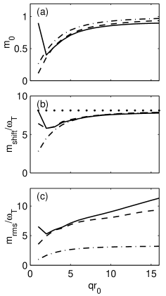
Figure 4: Spectral response function properties (see text) for a 3D condensate with $N_{0}U_{0}=10^{4}w_{0}$. $R(\mathbf{q},\omega)$ (solid), $R_{QH}(\mathbf{q},\omega)$ (dashed) and $I_{q}(\omega)$ (dash-dot). (a) the zeroth moment; (b) the mean response shift, with the shift $4\mu/7$ indicated (dotted); (c) the rms width of the frequency response. Bragg parameters are $V_{p}=0.2\omega_{T}$ and $T_{p}=0.4/\omega_{T}$.

Our numerical results lead to the following observations:

• In Fig. 4(a) the area under the response curve (i.e. $m_{0}$) is considered. The reduction of this from unity is characteristic of suppression of scattering for $q<q_{0}$ caused by the interference of the $u$ and $v$ amplitudes in the expression for the quasiparticle population (e.g. see Eq. (58)). Apart from the discrepancy at very low $q$ (which exists in all moments and which we discuss more fully below), both $I_{q}$ and $R_{QH}$ are in qualitatively good agreement with $R$. The finite pulse duration effect on $m_{0}$ is to reduce it uniformly from the $I_{q}$ prediction, a feature which $R_{QH}$ represents well.

• The mean shift (70) arises because of the Hartree interaction between the particles excited and those remaining in the condensate, as indicated by the Bogoliubov dispersion relation (55). The approximations $R_{QH}$ and $I_{q}$ are seen to be in good agreement with the full numerical calculation over most of the range of $q$, apart from $q=0$ (see below). At large values of $q$, the mean shift saturates at the value $4\mu/7$.

• The width prediction of $R_{QH}$ is in good agreement with the full numerical calculation at low $q$ ($2\leq qr_{0}\lesssim 6$), but differs as $q$ increases and the role of the condensate momentum distribution increases in importance. $I_{q}$ is in poor agreement for all $q$, because it ignores temporal broadening effects.

• In Fig. 4 the sharp features in the full numerical calculation of the moments of $R$ at extremely low $q$ arise because the (ground state) condensate momentum wavefunction has significant density in the region where the majority of the condensate is being scattered. This causes stimulated scattering of the condensate atoms, and will significantly affect the spectral response function when the amount of condensate initially present in the region we are scattering to is similar (or larger) than the amount of condensate excited with the Bragg pulse. This effect has been ignored in the derivation of $R_{QH}$ by taking $\hat{b}_{\mathbf{k}}$ to have a zero initial occupation in Eq. (57).

Evaluating condensate momentum width from the spectral response function

The MIT group have used the rms-width of the spectral response function to determine the Doppler width $\Delta\omega_{\mathrm{Dop}}$ of the condensate, and hence the momentum width $\sigma_{p}(=(m/q)$ $\Delta\omega_{\mathrm{Dop}}).$ This allowed them to make the important observation that the condensate coherence length is at least as large as the condensate size Stenger et al. (1999) (also see Stamper-Kurn and Ketterle (2001)). The Doppler width was obtained from the spectral response profile by assuming that the Doppler effect adds in quadrature to the density and temporal effects. The precise details of the procedure used in Stenger et al. (1999) are not given (see Fig. 3 of Stenger et al. (1999)), however an expression for the momentum width of the form

$$\sigma_{p}^{{}^{\prime}}=\frac{m\,\sqrt{m_{\mathrm{rms}}^{2}-(\Delta I_{q})^{2}-(\Delta F(\omega,T_{p}))^{2}}}{q},$$ (72)

is implied in the text. A difficulty that arises in applying Eq. (72) is that the rms-frequency spread $\Delta F(\omega,T_{p})$ due to the finite pulse length is ill defined. Formally $F(\omega,T_{p})$ has an unbounded rms-width, though the central peak has a half width of $\pi/T_{p}$. In order to allow the best possible result from the MIT procedure, we have treated $\Delta F$ as an arbitrary parameter, and fitted the function $\sigma_{p}^{{}^{\prime}}$ in Eq.(72) to the actual condensate momentum width of the ground state we use. The result for a range of $q$ values is shown plotted as circles in Fig. 5, and was obtained with a best fit value $\Delta F\approx 0.86\times\pi/T_{p}$. We can see that Eq. (72) does not give a particularly good estimate of the true momentum width, indicating that the assumption of quadrature contributions of density, momentum and finite time effects to the spectral response function is inappropriate. Agreement improves as $q$ increases, as would be expected, because the Doppler effect dominates over the other mechanisms in that regime.

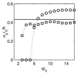
Figure 5: The true momentum width $\sigma_{p}$ of the condensate (solid line) in comparison to the estimated value from Eqs. (73) (squares) and (72) (circles). Other parameters as in Fig. 4.

Our approximate form $R_{QH}$ provides a more accurate means of extracting the Doppler width. We first assume that the finite time and density effects are well accounted for by $R_{QH},$ which has an an rms-width $\Delta R_{QH}$. We then assume that the overall width is obtained by adding this in quadrature to the Doppler width, which gives the following estimate $\tilde{\sigma}_{p}$ for the momentum width

$$\tilde{\sigma}_{p}=\frac{m\,\sqrt{m_{\mathrm{rms}}^{2}-(\Delta R_{QH})^{2}}}{q}$$ (73)

in which no fitting parameter is necessary. Results for $\tilde{\sigma}_{p}$ are also shown in Fig. 5 and clearly give a better estimate for the true width $\sigma_{p}$ than Eq. (72).

V.5 Scattering beyond the linear regime

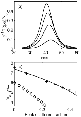
Figure 6: Laser intensity effects on the spectral response function. (a) Total scattered condensate fraction for $q=6/r_{0}$ and (lowest to highest) $V_{p}=0.51,\,0.85,\,1.1,\,1.3\,\omega_{T}.$ (b) Shift of peak response frequency $m_{\rm{shift}}$ as a function of the peak scattered fraction for $q=3/r_{0}$ (diamonds), $6/r_{0}$ (solid) and $9/r_{0}$ (crosses). Other parameters: spherically symmetric condensate, $N_{0}U_{0}=10^{4}w_{0},$ $q_{0}=3.8/r_{0}$ and $T_{p}=0.8/\omega_{T}$.

Spectroscopic experiments require that the number of atoms scattered be sufficient for the clear identification of momentum transfer to the system. In Stenger et al. (1999) the light intensity was chosen so that the largest amount of condensate scattered (at the Bragg resonance) was about $20\%$. The validity of the linear theories (e.g. section II) must be questioned at such large fractional transfers, where excitations can no longer be considered noninteracting (e.g. see Morgan et al. (1998)). The numerical GPE calculations do however remain valid in this regime, and can be used to understand the changes in the spectral response function that occur as the scattered fraction increases.

In Fig. 6 we present results which extend beyond the linear regime. In Fig. 6(a) we plot the scattered condensate fraction [$\gamma^{-1}R(\mathbf{q},\omega)/N_{0}]$ in a sequence of curves for increasing $V_{p}$. We have chosen to use the scattered condensate fraction rather than the spectral response function $R(\mathbf{q},\omega)$, since the numerical value of the scattered fraction indicates whether the measurement is outside the linear regime. This is shown clearly in this sequence of curves, which would simply be scaled by the ratios of $V_{p}^{2}$ if they were in the linear regime. Instead, we see that the shapes of the curves change as $V_{p}$ increases (and the scattered fraction increases) and in particular the peak frequency shifts downwards. In Fig. 6(b) we consider that dependence of the mean response frequency shift ($m_{\mathrm{shift}}$) on the peak scattered fraction of condensate (i.e. the fraction of condensate scattered at the Bragg resonance for the curves) for three different $q$ values. A number of features are apparent in those curves. First, the shift decreases below the linear prediction as the scattered fraction increases. Second, the decrease is larger for low momentum transfers ( $q<q_{0})$ than for higher momentum transfers. Third, for large enough momentum transfer, the shift at a given condensate fraction saturates

We note that in the MIT experiments a peak excitation fraction of $\sim 0.2$ was used Stenger et al. (1999). From Fig. 6 we see that even for the highest values of momentum transfer, (i.e. $q=6/r_{0}$ or $q=9/r_{0}$), the shift will be reduced by of order $15\%$ relative to the prediction of the linear theory.

VI Long time excitation: energy response

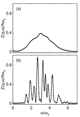
Figure 7: Energy response function calculated for a two dimensional condensate and a Bragg grating with $q=1/r_{0}$ and duration (a) $T_{p}=2\pi/\omega_{T}$ and (b) $T_{p}=10\pi/\omega_{T}$. In both cases the intensity is chosen so that $\gamma^{-1}\approx 0.05N_{0}$.

As discussed in section III, momentum is not a conserved quantity in a trapped condensate, and is not a convenient observable for the long time limit. Here we investigate the energy transfer to the condensate by Bragg excitation (see also Brunello et al. (2001)), since in the unperturbed system (i.e. in the absence of the Bragg grating) energy is a conserved quantity. A possible method of measuring the energy transferred is the technique of calorimetry, which has been applied by the Ketterle group in a somewhat different context Wol .

We define an energy response function $Z(\mathbf{q},\omega)$ analogous to the (momentum) spectral response function by the equation

$$Z(\mathbf{q},\omega)\equiv\gamma\,\left[E[\Psi(\mathbf{r},T_{p})]-E[\Psi(\mathbf{r},t=0)]\right],$$ (74)

where

$$E[\Psi]=\int d\mathbf{r}\,\left[\Psi^{*}\left[-{\hbar^{2}\over 2m}\nabla^{2}+V_{T}(\mathbf{r})\right]\Psi+{U_{0}\over 2}|\Psi|^{4}\right],$$ (75)

is the energy functional and $\gamma$ is defined in Eq. (36). Thus $Z(\mathbf{q},\omega)$ is the rate of energy transfer to the condensate from a Bragg grating of frequency $\omega$ and wave vector $\mathbf{q}$. The results of section II for the quasiparticle evolution can be readily applied to evaluating Eq. (74). Using the $T=0$K results of either the vacuum expectation of the Bogoliubov Hamiltonian in Eq. (14) with $\hat{b}_{i}$ given by (19), or the linearized Gross-Pitaevskii result (28) in the energy functional (75) gives

$$E[\Psi(\mathbf{r},t)]=E_{0}+\sum_{i}\hbar\omega_{i}\langle\hat{n}_{i}(t)\rangle,$$ (76)

where $E_{0}=E[\sqrt{N_{0}}\psi_{0}]$ is the initial (ground state) energy and $\langle\hat{n}_{i}(t)\rangle$ is the Bragg induced quasiparticle occupation (30) at time $t$. Substituting Eq. (76) into Eq. (74) gives

$$Z(\mathbf{q},\omega)=\gamma\sum_{i}\hbar\omega_{i}\langle\hat{n}_{i}(T_{p})\rangle.$$ (77)

As noted above, because energy is a constant of motion of the trapped condensate, we can take $T_{p}\gg 2\pi/\omega_{T}$ (though we require $V_{p}^{2}T_{p}$ to remain small compared to unity for our linear analysis to remain valid) and from Eq. (32) (with $\langle\hat{n}_{i}(0)\rangle=0$), we have

$$Z(\mathbf{q},\omega)=\sum_{i}\hbar\omega_{i}\left|\int d\mathbf{r}(u^{*}_{i}+v^{*}_{i})e^{i\mathbf{q}\cdot\mathbf{r}}|\psi_{0}|\right|^{2}F(\omega_{i}-\omega,T_{p}).$$ (78)

Thus in long duration (weak) Bragg excitation, the only contribution to $Z(\mathbf{q},\omega)$ will come from quasiparticle states with energy approximately matching $\hbar\omega$ (see Eq. (34)).

In Fig. 7 we present results for the energy response function of a 2D condensate for two different durations of Bragg excitation. Fig. 7(a) shows the case of Bragg excitation applied for a single trap period ($T_{p}=2\pi/\omega_{T}$). In this case the frequency spread of the Bragg pulse is sufficiently wide that only a single broad peak of energy absorption is discernible from the condensate i.e. the functions $F(\omega-\omega_{i},T)$ appearing in summation of Eq. (78) are sufficiently broad in frequency space to allow a large number of quasiparticles to respond. In Fig. 7(b) $Z(\mathbf{q},\omega)$ is shown for the case of a Bragg pulse applied for five trap periods ($T_{p}=10\pi/\omega_{T}$). Here the detailed structure of the energy response function is revealed, with individual (possibly degenerate) quasiparticle peaks being visible. We emphasize that current momentum response experiments (i.e. $R(\mathbf{q},\omega)$) are essentially limited to at most a quarter trap period of excitation.

A response measurement such as shown in Fig. 7(b) reveals a wealth of information about the nature of the condensate excitation spectrum. The frequencies ($\omega_{i}$) of the quasiparticles can be determined by the location of the resonant peaks of the response function, and these frequency peaks become narrower and better defined as $T_{p}$ increases. We note that for a given peak corresponding to a Bragg frequency $\omega_{p}$, the area under the peak is equal to the matrix element

$$\int_{\delta\omega}d\omega\,Z(\mathbf{q},\omega)=\sum_{i\,(\omega_{i}\in\delta\omega)}\hbar\omega_{i}\left|\int d\mathbf{r}(u^{*}_{i}+v^{*}_{i})e^{i\mathbf{q}\cdot\mathbf{r}}|\psi_{0}|\right|^{2},$$ (79)

where $\delta\omega$ ($\approx[\omega_{p}-\pi/T_{p},\omega_{p}+\pi/T_{p}]$) is the frequency width of the pulse and the summation is taken over quasiparticles in the energy range $\delta\omega$.

VII Discussion

In this paper we have given a detailed theoretical analysis of the phenomenon of Bragg spectroscopy from a Bose-Einstein condensate. We began by deriving analytic expressions for the evolution of the quasiparticle operators, which contain all possible information about the system in the linear response regime. We then demonstrated that at $T=0$K, the mean values of the quasiparticle operators are identical to the quasiparticle amplitudes obtained by solving the linearised Gross-Pitaevskii equation. Thus, for the purpose of calculating the observable of the Bragg spectroscopy experiments (the transferred momentum), a meanfield treatment is equivalent to the full quantum treatment. Consequently, we based our detailed analysis of Bragg spectroscopy on the meanfield equation for Bragg scattering presented in a previous paper. The central object for the experiments is the spectral response function for the momentum transfer, $R(\mathbf{q},\omega).$ We derived the relationship between $R(\mathbf{q},\omega)$ and the dynamic structure factor and showed that, contrary to the assumptions of previous analyses, there is no regime in which the two quantities are equivalent for trapped condensates.

The results of our numerical simulations of Bragg spectroscopy, which were carried out in axially symmetric three-dimensional cases, or in two dimensions, were characterised by the behaviour of $R(\mathbf{q},\omega)$. These full numerical solutions are accurate for all values of $q$ that can be resolved by the computational grid, however the computationally intensive nature of the calculation made quantitative comparison of our theory with the MIT experiments difficult. The analytic approximation for the spectral response function, $R_{QH}(\mathbf{q},\omega)$, provides a means of extending the regime of comparison to large condensates, and systems without axial symmetry, and we showed that it accurately represents $R(\mathbf{q},\omega)$, except in those regimes where the momentum width is dominant ($\sigma_{p}q/m$ exceeds $\pi/T_{p}$ and $\mu$) or where stimulated effects can occur ($\hbar q<\sigma_{p}$). It also provided a means for identifying the relative importance of three broadening and shift mechanisms (meanfield, Doppler, and finite pulse duration). We have shown that the suppression of scattering at small values of $q$ observed by Stamper-Kurn et al. Stamper-Kurn et al. (1999) is accounted for by the meanfield treatment, and can be interpreted in terms of the interference of the $u$ and $v$ quasiparticle amplitudes.

A remaining point to emphasize is that our numerical calculations allowed us to investigate the regime of large laser intensities where the linear response condition is invalid. We found that a significant decrease in the shift of the spectral response function can occur due to depletion of the initial condensate.

Bogoliubov conventions

Several different forms of the Bogoliubov transformation have been used in the theoretical description of inhomogeneous Bose-Einstein condensates. These transformations typically differ in their choice of sign between the $u$ and $v$ amplitudes, and by the explicit inclusion of phase. To assist comparison of our results to the work of others, we summarize four different definitions, and show how the form of the quasiparticle population result (Eq. (30)) is altered by each choice. In section II.1.1 we used the orthogonal quasiparticle basis, since the Bogoliubov diagonalization of the many-body Hamiltonian must be made with excitations that are orthogonal to the ground state. However, the quasiparticle population result, Eq. (30), is insensitive to this and so for brevity we will use the non-orthogonal basis states.

In what follows we denote our choice of quasiparticle amplitudes by the notation $\{u^{(+)}_{i},v_{i}^{(+)}\}$. These are closely related to the form used in Fetter (1996) by Fetter (which we denote $\{u^{(-)}_{i},v_{i}^{(-)}\}$), but differ by a minus sign in the relative phase between $u_{i}$ and $v_{i}$. Both these conventions explicitly include the condensate phase, and the operator part of the field operator is expanded in the form

$$\hat{\phi}=e^{iS_{0}(\mathbf{r})}\sum_{i}\left[u^{(\pm)}_{i}(\mathbf{r})\hat{b}_{i}(t)\pm v_{i}^{(\pm)*}(\mathbf{r})\hat{b}_{i}^{\dagger}(t)\right],$$ (80)

where the quasiparticles modes obey the equations (at $T=0$K with $N_{0}$ particles in the $\psi_{0}$ state)

$${\cal L}u^{(\pm)}_{i}\pm N_{0}U_{0}|\psi_{0}|^{2}v_{i} = \hbar\omega_{i}u^{(\pm)}_{i},$$ (81)

$${\cal L}^{*}v^{(\pm)}_{i}\pm N_{0}U_{0}|\psi_{0}|^{2}u^{(\pm)}_{i} = -\hbar\omega_{i}v^{(\pm)}_{i},$$ (82)

and ${\cal L}$ is as defined in Eq. (11). The basis choice of Eqs. (81) and (82) leads to the vacuum expectation value Eq. (29) having the form

$$\langle\hat{b}_{i}(t)\rangle = -i\sqrt{N_{0}}\int_{0}^{t}dt^{\prime}\,V(t^{\prime})e^{i\omega_{i}t^{\prime}}\int d\mathbf{r}\,(u^{(\pm)*}_{i}\pm v^{(\pm)*}_{i})$$ (83)

$$\times\cos(\mathbf{q}\cdot\mathbf{r}-\omega t)|\psi_{0}|.$$

The most common form of the Bogoliubov transformation (e.g. see Griffin (1996); Morgan et al. (1998)), uses the following form for the expansion of the operator part of the field

$$\hat{\phi}=\sum_{i}\left[\bar{u}^{(\pm)}_{i}(\mathbf{r})\hat{b}_{i}(t)\pm\bar{v}_{i}^{(\pm)*}(\mathbf{r})\hat{b}_{i}^{\dagger}(t)\right],$$ (84)

where the $\pm$ indices indicate the relative choice of sign between the $u$ and $v$ terms in Eq. (84). These quasiparticles modes obey the equations (at $T=0$K with $N_{0}$ particles in the $\psi_{0}$ state)

$$L\bar{u}^{(\pm)}_{i}\pm N_{0}U_{0}|\psi_{0}|^{2}\bar{v}^{(\pm)}_{i} = \hbar\omega_{i}\bar{u}^{(\pm)}_{i},$$ (85)

$$L\bar{v}^{(\pm)}_{i}\pm N_{0}U_{0}|\psi_{0}|^{2}\bar{u}^{(\pm)}_{i} = -\hbar\omega_{i}\bar{v}^{(\pm)}_{i},$$ (86)

where $L$ is defined as

$$L=\left[-{\hbar^{2}\over 2m}\nabla^{2}+V_{T}(\mathbf{r})-\hbar\mu+2N_{0}U_{0}|\psi_{0}|^{2}\right].$$ (87)

In this case the mean value of $\hat{b}_{i}$ is

$$\langle\hat{b}_{i}(t)\rangle = -i\sqrt{N_{0}}\int_{0}^{t}dt^{\prime}\,V(t^{\prime})e^{i\omega_{i}t^{\prime}}$$

$$\times\int d\mathbf{r}\,(\bar{u}^{(\pm)*}_{i}\psi_{0}\pm\bar{v}^{(\pm)*}_{i}\psi_{0}^{*})\cos(\mathbf{q}\cdot\mathbf{r}-\omega t),$$

(see Eq. (29)). When $\psi_{0}$ is a ground state (i.e. has constant phase), $\psi_{0}$ can be taken as real in Eq. (Bogoliubov conventions), i.e.

$$\langle\hat{b}_{i}(t)\rangle = -i\sqrt{N_{0}}\int_{0}^{t}dt^{\prime}\,V(t^{\prime})e^{i\omega_{i}t^{\prime}}$$

$$\times\int d\mathbf{r}\,(\bar{u}^{(\pm)*}_{i}\pm\bar{v}^{(\pm)*}_{i})\cos(\mathbf{q}\cdot\mathbf{r}-\omega t)\psi_{0}.$$

References

- Stenger et al. (1999) J. Stenger, S. Inouye, A. P. Chikkatur, D. M. Stamper-Kurn, D. E. Pritchard, and W. Ketterle, Phys. Rev. Lett. 82, 4569 (1999).
- Stamper-Kurn et al. (1999) D. M. Stamper-Kurn, A. P. Chikkatur, A. Gorlitz, S. Inouye, S. Gupta, D. E. Pritchard, and W. Ketterle, Phys. Rev. Lett. 83, 2876 (1999).
- Pines and Nozieres (1966,1990,1999) D. Pines and P. Nozieres, The Theory of Quantum Liquids, vol. I (Benjamin, New York, 1966,1990,1999).
- Pines and Nozieres (1990,1999) D. Pines and P. Nozieres, The Theory of Quantum Liquids, vol. II (Benjamin, New York, 1990,1999).
- Griffin (1993) A. Griffin, Excitations in a Bose-Condensed Liquid, no. 4 in Cambridge Studies in Low Temperature Physics (Cambridge University Press, N. Y., 1993).
- Stamper-Kurn and Ketterle (2001) D. M. Stamper-Kurn and W. Ketterle, in Coherent Atomic Matter Waves, Les Houches Summer School Session LXXII in 1999, edited by R. Kaiser, C. Westbrook, and F. David (Springer, New York, 2001), vol. 72, p. 137.
- Blakie and Ballagh (2000) P. B. Blakie and R. J. Ballagh, J. Phys. B 33, 2961 (2000).
- Zambelli et al. (2000) F. Zambelli, L. Pitaevskii, D. M. Stamper-Kurn, and S. Stringari, Phys. Rev. A 61, 063608 (2000).
- Brunello et al. (2001) A. Brunello, F.Dalfovo, L. Pitaevskii, S. Stringari, and F. Zambelli, Momentum transferred to a trapped Bose-Einstein condensate by stimulated light scattering, cond-mat/0104051 (2001).
- Brunello et al. (2000) A. Brunello, F. Dalfovo, L. Pitaevskii, and S. Stringari, Phys. Rev. Lett. 85, 4422 (2000).
- Pitaevskii and Stringari (1999) L. Pitaevskii and S. Stringari, Phys. Rev. Lett. 83, 4237 (1999).
- Griffin (1996) A. Griffin, Phys. Rev. B 53, 9341 (1996).
- Fetter (1972) A. L. Fetter, Ann. Phys. 70, 67 (1972).
- Morgan et al. (1998) S. A. Morgan, S. Choi, K. Burnett, and M. Edwards, Phys. Rev. A 57, 3818 (1998).
- Gardiner and Zoller (1999) C. W. Gardiner and P. Zoller, Quantum Noise, Springer Series in Synergetics (Springer Verlag, Berlin, 1999), 2nd ed., see page 105.
- Hutchinson et al. (1997) D. A. W. Hutchinson, E. Zaremba, and A. Griffin, Phys. Rev. Lett. 78, 1842 (1997).
- Hutchinson et al. (1998) D. A. W. Hutchinson, R. J. Dodd, and K. Burnett, Phys. Rev. Lett. 81, 2198 (1998).
- Morgan (2000) S. A. Morgan, J. Phys. B 33, 3847 (2000).
- Davis et al. (2001) M. J. Davis, S. A. Morgan, and K. Burnett, Phys. Rev. Lett. 87, 160402 (2001).
- Csordás et al. (1996) A. Csordás, R. Graham, and P. Sźepfalusy, Phys. Rev. A 54, R2543 (1996).
- Fetter and Rokhsar (1998) A. L. Fetter and D. Rokhsar, Phys. Rev. A 57, 1191 (1998).
- Wu and Griffin (1996) W. Wu and A. Griffin, Phys. Rev. A 54, 4204 (1996).
- van Hove (1954) L. van Hove, Phys. Rev. 95, 249 (1954).
- Javanainen (1995) J. Javanainen, Phys. Rev. Lett. 75, 1927 (1995).
- Blakie and R. J. Ballagh (2001) P. B. Blakie and R. J. Ballagh, Phys. Rev. Lett. 86, 3930 (2001).
- (26) C. Raman et al., J. Low Temp. Phys. 122, 99 (2001); R. Onofrio et al., Phys. Rev. Lett. 85, 2228 (2000).
- Fetter (1996) A. L. Fetter, Phys. Rev. A 53, 4245 (1996).