Resonant Raman Scattering by Charge Density and Single Particle Excitations in Semiconductor Nanostructures: A Generalized Interband-Resonant Random-Phase-Approximation Theory

Abstract

We develop a generic theory for the resonant inelastic light (Raman) scattering by a conduction band quantum plasma taking into account the presence of the filled valence band in doped semiconductor nanostructures within a generalized resonant random phase approximation (RPA). Our generalized RPA theory explicitly incorporates the two-step resonance process where an electron from the filled valence band is first excited by the incident photon into the conduction band before an electron from the conduction band falls back into the valence band emitting the scattered photon. We show that when the incident photon energy is close to a resonance energy, i.e. the valence-to-conduction band gap of the semiconductor structure, the Raman scattering spectral weight at single particle excitation energies may be substantially enhanced even for long wavelength excitations, and may become comparable to the spectral weight of collective charge density excitations (plasmon). Away from resonance, i.e. when the incident photon energy is different from the band gap energy, plasmons dominate the Raman scattering spectrum. We find no qualitative difference in the resonance effects on the Raman scattering spectra among systems of different dimensionalities (one, two and three) within RPA. This is explained by the decoherence effect of the resonant interband transition on the collective motion of conduction band electrons. Our theoretical calculations agree well (qualitatively and semi-quantitatively) with the available experimental results, in contrast to the standard nonresonant RPA theory which predicts vanishing long wavelength Raman spectral weight for single particle excitations.

I Introduction

In recent years the elementary electronic excitation spectra of a variety of doped semiconductor nanostructures, such as two dimensional (2D) quantum wells (QW) heterostructures, superlattices, and more recently, one dimensional (1D) quantum wire (QWR) systems, have been studied extensively both experimentally [1, 2, 3, 4, 5, 6, 7, 8, 9, 10, 11] and theoretically [12, 13, 14, 15, 16, 17, 18, 19]. Rich experimental spectra of the elementary electronic excitations (such as charge density excitations (CDE), spin density excitations (SDE), and single particle excitations (SPE), for both intrasubband and intersubband excitations) in these systems are typically experimentally investigated by using the resonant Raman scattering (RRS) technique, which is a powerful and versatile spectroscopic tool to study interacting electron systems. In the RRS experiment, external photons are absorbed at one frequency and momentum, $\omega_{i}$ and $\mathbf{k}\it_{i}$, and emitted at another, $\omega_{f}$ and $\mathbf{k}\it_{f}$, creating one or more particle-hole pair (or collective) excitations in the conduction band. The energy and momentum difference between the incident photon and the scattered photon is Stokes shift, indicating the dispersion of the relevant elementary electronic excitation created in the system. In the so-called polarized RRS geometry with the incident and scattered photons having the same polarization, the excited electrons have no spin flips during the scattering process, which therefore corresponds to the elementary charge density excitations of the system. At low temperatures (which is of interest to us in this paper) there is no real absorption of elementary excitations by the incident photon and the anti-Stokes line is not of any importance. (We use $\hbar=1$ throughout this paper.)

In the standard theory [16, 17, 18, 19, 20], which ignores the role of the valence band and simplistically assumes the external photons to be interacting entirely with conduction band electrons, the polarized RRS intensity is proportional to the dynamical structure factor [20, 21] of the conduction band electrons and therefore has strong spectral peaks at the collective mode frequencies at the wavevectors defined by the experimental geometry. The dynamical structure factor peaks correspond to the poles of the reducible density response function, which are given by the collective CDEs (plasmons) of the electron system in the long wavelength limit. In particular, the single particle electron-hole excitations, which are at the poles of the corresponding irreducible response function, carry no long wavelength spectral weight (about three orders of magnitude weaker than the CDE spectral weight at the typical wavevector, $10^{5}$ cm^-1, accessible in RRS experiments) in the density response function (according to the $f$-sum rule [20]). The SPE therefore should not, as a matter of principle, show up in the polarized RRS spectra in any dimensions. The remarkable experimental fact is that there is always a relatively weak (but quite distinct) SPE peak in the observed polarized RRS spectra in addition to the expected CDE peak. This experimental presence of SPE peak in RRS cannot be explained by the standard theory, which, however, does give the correct mode dispersion energy for both the CDE and the SPE, but fails to explain why the SPE spectral weight is strongly enhanced in the RRS experiments. This puzzling feature [1, 2, 19] of an ubiquitous anomalous SPE peak in addition to the expected CDE peak (or equivalently a two-peak structure) occurs in one, two, and even in three dimensional doped semiconductor nanostructures [4]. It exists in low dimensional semiconductor systems both for intrasubband and intersubband excitations.

Many theoretical proposals [12, 13, 14, 15, 22, 23] have been made to explain this two-peak RRS puzzle. $Ad$ $hoc$ proposals [5, 22] have been made in the literature that perhaps a serious breakdown of momentum or wavevector conservation (arising, for example, from scattering by random impurities) is responsible for somehow transferring spectral weight from large to small wavevectors, because the usual linear response theory predicts that at very large wavevectors (an order of magnitude larger than the experimentally used RRS wavevectors), where the CDE mode is severely Landau damped, the dynamical structure factor should contain finite SPE spectral weight corresponding to high energy electron-hole excitations. Apart from being completely $ad$ $hoc$, this proposal also suffers from any lack of empirical evidence in its support — in particular, the observed anomalous SPE peak in the RRS spectra does not correlate with the strength of the impurity scattering in the system. We have recently systematically analyzed [15] all the proposed mechanisms within the non-resonant RRS theory (i.e. without incorporating the valence band in the theory, assuming simply the inelastic light scattering process to be entirely confined to the conduction band free carrier system) leading to the conclusion that none of the proposed nonresonant mechanisms can explain the ubiquitous two-peak (the lower energy SPE peak and the higher energy CDE peak) structure of the observed RRS spectra.

We have recently reported [12] in a short letter a new resonant RRS theory by generalizing the nonresonant RPA theory to include the filled valence band in the semiconductor, reflecting the two-step resonant nature of the RRS process. The purpose of the current article is to provide the details of our resonant RRS theory, and more importantly, to present RRS results for 2D and 3D systems which have not been discussed earlier in the literature (our earlier letter [12] presented only 1D RRS results). The observed experimental RRS phenomenology in 1D, 2D, and 3D systems being very similar qualitatively, our generic interband-resonant RRS theory, as reported herein, provides the conceptual theoretical foundation for understanding RRS spectroscopy in doped semiconductor structures.

In this context, we emphasize that the striking similarity of the experimental RRS spectra in one, two, and three dimensional semiconductor systems suggests that the problem (namely, the two peak nature of the RRS spectra with the conspicuous presence of the ”forbidden” SPE peak) is not specific to 1D systems, where our earlier theory [12] was applied. The ubiquitousness of the strong SPE spectral weight in the RRS experiment (independent of system dimensionality, dependent only on the resonant nature of the experiment) suggests that the theoretical explanation for this puzzle must arise from some generic physics underlying RRS itself, and cannot be explained by the non-generic and manifestly system-specific theories which have been made occasionally in the literature. The resonant RRS theory presented herein (and in our short letter) provides a generic explanation for the two-peak structure of the RRS spectra by establishing that the so-called low energy anomalous SPE feature in the RRS spectrum arises entirely from the resonant two-step nature of the RRS experiment, and cannot be the explained within any non-resonant theory.

In this paper we provide (within the resonant RPA scheme) the compellingly generic theory for RRS experiments by including the valence band electrons during the scattering processes for one, two and three dimensional semiconductor systems, following our earlier short paper [12] on 1D systems. We find that the RRS spectral weight at SPE energy is a strong function of the resonance condition — the SPE spectral weight is substantially enhanced when the incident photon frequency is near the semiconductor band gap resonance energy, and decreases drastically away from the resonance. It is important to emphasize that this feature of our theory agrees with experimental observations — the anomalous SPE peak exists only around resonance and its spectral strength decreases off resonance. Our results show similar qualitative behavior for the RRS spectra in one, two and three dimensional systems.

One dimensional systems [24] actually pose a special (and subtle) problem with respect to understanding the two-peak RRS spectra because 1D electron systems are generically [25, 26] Luttinger liquids (i.e. non-Fermi liquids) which have no quasiparticle (SPE) excitations whatsoever. The elementary excitations in 1D electron systems are bosonic spinon and holon collective modes. It is therefore conceptually problematic to comprehend how an anomalous ”SPE” feature can arise in 1D semiconductor quantum wire RRS spectra as has been experimentally observed [1, 2, 3, 10, 11]. The issue of understanding 1D RRS spectra from a Luttinger liquid viewpoint has been recently discussed [13, 14, 15] in the literature, and we refrain from further discussing this point in this article since this is beyond the scope of our work. In particular, our use of generalized RPA enables us to develop a unified consistent theory of resonant RRS in arbitrary dimensions (including 1D), and the Luttinger liquid nature of 1D quantum wires is not of any relevance in our theory. We mention, however, that a complete Luttinger liquid theory of 1D RRS experiments has recently been developed [14], and this Luttinger liquid theory builds on the resonant nature of our work presented in this article.

The rest of this paper is organized as follows: in Sec. II we describe the theory of nonresonant and resonant Raman scattering process in RPA; in Sec. III we present and discuss our calculated RRS results for one, two, and three dimensional GaAs semiconductor systems; we then summarize our work in Sec. IV. All the results shown in this paper are for GaAs-based systems, but obviously the theory applies to any direct band gap semiconductor material.

II Theory

In Fig. 1(a) we depict the schematic diagram [12, 27, 28, 29] for the two step process (steps 1 and 2 in the figure) involved in the polarized resonant Raman scattering spectroscopy at the $E_{0}+\Delta_{0}$ direct gap of electron doped GaAs system [29] where an electron in the valence band is excited by the incident photon into an excited (i.e. above the Fermi level) conduction band state, leaving a valence band hole behind (step 1); then an electron from inside the conduction band Fermi surface recombines with the hole in the valence band (step 2), emitting an outgoing photon with an energy and momentum (Stokes) shift. The RRS process is a two-step process involving steps 1 and 2 with the net result of there being an elementary electron excitation created in the conduction band through intermediate valence band states as shown in Fig. 1. The non-resonant approximation to RRS ignores the intermediate valence band states and approximates the RRS process to be taking place entirely within the conduction band of the system, as shown by the step 3 in Fig. 1. The whole point of the theory [12] developed in this paper is that the non-resonant step 3 is not equivalent to the resonant scattering involving steps 1 and 2. Note that the resonant process involving steps 1 and 2 explicitly depends on the incident photon energy, while the non-resonant approximation depicted in step 3 depends only on the energy difference between the incident and the scattered photons and not on the incident photon energy. This difference turns out to be crucial in the RRS theory, and the resonance condition in the incident photon energy gives rise to the anomalous SPE-like feature in the RRS spectra as shown below. Electron spin is conserved throughout the scattering processes since we are considering only the polarized geometry where no spin flip occurs. As mentioned before we use the random phase approximation (RPA) in our theory taking care to generalize it to the resonant situation involving steps 1 and 2. In the RPA one neglects all exchange-correlation effects (e.g. self-energy and vertex corrections due to electron-electron interaction), including only the long range Coulomb interaction $V_{c}(\mathbf{q}\it)$ in the dynamical screening by the electron system so as to correct the noninteracting irreducible response function to the reducible response function. Following a preliminary discussion of the Coulomb interaction in 1, 2 and 3 dimensional semiconductor system in subsection A below, we then develop the nonresonant and the resonant RRS theories in sections B and C respectively. Our theory is entirely within the effective mass approximation, and we parameterize the electron system in the semiconductor by electron ($m_{e}$) and hole ($m_{h}$) effective masses corresponding to the top (bottom) of the conduction (valence) band and by a background lattice dielectric constant $\varepsilon_{0}$.

A Coulomb Interaction

The realistic (bare) Coulomb interaction in the artificially confined semiconductor nanostructures depends strongly on the confinement geometry of the systems. In the bulk 3D semiconductor materials, the unscreened Coulomb interaction has a long-ranged $1/r$ decay in the real space, and has the following Fourier transform in momentum space:

$$V^{\rm{3D}}_{c}(\mathbf{q}\it)=\frac{e^{\rm 2}}{\varepsilon_{0}}\int\frac{{d}\mathbf{r}\it^{\rm{3}}}{|\mathbf{r}\it|}e^{{i}\mathbf{q}\it\cdot\mathbf{r}\it}=\frac{\rm{4}\pi\it e^{\rm 2}}{\varepsilon_{\rm{0}}|\mathbf{q}\it|^{\rm{2}}},$$ (1)

where $e$ is the electron charge and $\varepsilon_{0}$ is the dielectric constant of the background material (about 12 in the GaAs semiconductor system). We use the static ($\varepsilon_{0}$) lattice dielectric constant in our theory rather than the more conventional high frequency ($\varepsilon_{\infty}$) dielectric constant in defining the Coulomb interaction, $V_{c}(\mathbf{q}\it)$, because inclusion of $\varepsilon_{0}$ is known to approximately account for the polaronic electron-phonon interaction in the system, which is rather weak in GaAs because of its low Fr$\ddot{\rm o}$hlich coupling constant ($\sim 0.07$). In the 2D semiconductor quantum well system, modern fabrication techniques have produced very narrow 2D wells (of nanostructure size $<100$ Å in GaAs in the confinement direction), leading to an almost pure 2D electron system. It is therefore a good approximation to assume the well width to be zero in our calculation, giving a 2D Fourier transform of the Coulomb interaction:

$$V^{\rm{2D}}_{c}(\mathbf{q}\it)=\frac{e^{\rm 2}}{\varepsilon_{0}}\int\frac{{d}\mathbf{r}\it^{\rm{2}}}{|\mathbf{r}\it|}e^{{i}\mathbf{q}\it\cdot\mathbf{r}\it}=\frac{\rm{2}\pi\it{e}^{\rm 2}}{\varepsilon_{\rm{0}}|\mathbf{q}\it|}.$$ (2)

Inclusion of the confinement wavefunction effect in the theory is straightforward and leads to a form factor $f(\mathbf{q}\it)$ ($<1$) multiplying $V_{c}^{\rm{2D}}(\mathbf{q}\it)$ in the theory. For the 1D semiconductor quantum wire system, we have to consider the realistic finite width of the wire (i.e. the relevant 1D form factor effect) because the 1D Fourier transform of $1/r$ potential (i.e. $\int dre^{iqr}/|r|$) diverges logarithmically requiring regularization by a length cut-off associated with the typical confinement size. Therefore the Coulomb interaction for the finite width quantum wire is obtained by taking the expectation value of the 2D Coulomb interaction (assuming the width in the $z$ direction to be zero for simplicity as in our 2D model in Eq. 2) over the confinement wavefunction along the transverse direction ($y$) of the wire. We then have [30] the following Coulomb interaction matrix element in the 1D QWR structure of finite width:

$$V^{\rm{1D}}_{c,ij}(q) = \frac{e^{\rm 2}}{\varepsilon_{0}}\int_{-\infty}^{\infty}\it{}dy\,dy^{\prime}\int_{-\infty}^{\infty}dx\frac{e^{-iqx}|\phi_{i}(y)|^{\rm 2\it}|\phi_{j}(y^{\prime})|^{\rm 2\it}}{\sqrt{x^{\rm 2\it}+(y-y^{\prime})^{\rm 2\it}}}$$ (3)

$$= \frac{2e^{\rm 2}}{\varepsilon_{0}}\int_{-\infty}^{\infty}\it{}dy\,dy^{\prime}|\phi_{i}(y)|^{\rm 2\it}|\phi_{j}(y^{\prime})|^{\rm 2\it}K_{\rm 0}(q|y-y^{\prime}|^{2}),$$ (4)

for interaction between electrons of subband $i$ and subband $j$. $\phi_{i}(y)$ is the electron wavefunction of $i$th subband of the QWR along the transverse direction. In this paper we assume that only the lowest ($i=1$) ground conduction subband is occupied (i.e. subband spacing $\Delta E_{12}>E_{F}$ at zero temperature and all the higher energy subbands are empty) and neglect any intersubband transition, so that the subband index $i=1$ throughout and will not be explicitly shown. $K_{0}(x)$ in Eq. (3) is the zeroth-order modified Bessel function of the second kind. The exact form of wavefunction $\phi(y)$ depends on the confinement geometry of the QWR system. For simplicity we assume the QWR confinement potential to be the 1D infinite square well in the $y$ direction. This turns out to be a good approximation for the electrostatic gate-controlled confinement in the presence of the self-consistent Hartree potential due to the free electrons themselves [30]. The the confinement wavefunction $\phi(y)$ is (for the ground subband):

$$\phi(y)=\left\{\begin{array}[]{ll}\sqrt{\frac{\displaystyle 2}{\displaystyle a}}\cos\left(\frac{\displaystyle\pi y}{\displaystyle a}\right)&\mbox{if}-a/2<y<a/2\\ 0&\rm{otherwise},\end{array}\right.$$ (7)

where $a$ is the wire width in the $y$ direction. Using Eqs. (3) and (4) we can numerically calculate the effective 1D Coulomb interaction [30] for the semiconductor QWR system. Unlike the power-law behavior of Coulomb interaction in the higher dimensions (Eqs. (1) and (2)), $V^{\rm{1D}}_{c}(q)$ has a weak logarithmic divergence, $-2{e}^{2}\ln(qa)/\varepsilon_{0}$, in the long wavelength limit ($q\rightarrow 0$). Because of this logarithmic dependence of $V_{c}(q)$ on $q$ (as $q\rightarrow 0$), the precise value of the wire width ($a$) is not particularly important in our theory, making our simple infinite square well approximation a reasonable one for our purpose.

B Nonresonant Raman scattering

In the presence of an external photon field the interacting Hamiltonian between the free electron gas and the radiation field is assumed to be obtainable from the standard gauge-invariant prescription [31, 32], $\mathbf{p}\it\rightarrow\mathbf{p}\it-e\mathbf{A}\it/c$, where $\mathbf{A}\it$ is the radiation field (photon) vector potential operator and $c$ the speed of light. The Hamiltonian including the radiation field and the electrons (i.e. the free carriers induced by doping) in the semiconductor conduction band can therefore be written as (we neglect the spin-photon interaction considering only polarized RRS spectra where spins do not play any explicit role)

$$H = \sum_{i}^{N}\frac{1}{2m_{e}}\left(\mathbf{p}\it_{i}-e\mathbf{A}\it(\mathbf{x}\it_{i},t)/c\right)^{2}+\sum^{N}_{ij,i>j}V_{c}(\mathbf{x}\it_{i}-\mathbf{x}\it_{j})$$ (8)

$$= \underbrace{\sum_{i}^{N}\left[\frac{\mathbf{p}\it_{i}^{\rm 2}}{2m_{e}}+\sum^{N}_{j<i}V_{c}(\mathbf{x}\it_{i}-\mathbf{x}\it_{j})\right]}_{\displaystyle H_{0}}+\underbrace{\sum_{i}^{N}\left[-\frac{e}{m_{e}c}\mathbf{p}\it_{i}\cdot\mathbf{A}\it(\mathbf{x}\it_{i},t)+\frac{e^{\rm 2}}{\rm 2\it m_{e}c^{\rm 2}}\mathbf{A}\it(\mathbf{x}\it_{i},t)^{\rm 2}\right]}_{\displaystyle H_{I}}$$ (9)

in the effective mass approximation with $m_{e}$ being the effective electron mass of the semiconductor conduction band. We have made the transverse gauge choice [31], $\nabla\cdot\mathbf{A}\it(\mathbf{x}\it_{i},t)=\rm{0}$, for the radiation field, leading to $\mathbf{p}\it_{i}\cdot\mathbf{A}\it=\mathbf{A}\it\cdot\mathbf{p}\it_{i}$ as used in Eq. (5). $H_{0}$ is the Hamiltonian of electrons interacting with Coulomb potential without the radiation field, and $H_{I}$ is the electron-photon interaction Hamiltonian which plays a crucial role in the Raman scattering problem. Figs. 1(b) and 1(c) correspond to the scattering processes induced by the linear ($\mathbf{p}\it\cdot\mathbf{A}\it$) term and the quadratic ($\mathbf{A}\it^{\rm 2}$) term respectively in the second quantization representation. The $\mathbf{p}\it\cdot\mathbf{A}\it$ term creates and annihilates one photon in the state it acts on, having no contribution to the scattering rate in the first order time-dependent perturbation theory since there is no net change of photon numbers. The quadratic $\mathbf{A}\it^{\rm 2}$ term, on the other hand, gives a non-vanishing first order contribution to the scattering rate because photons are created and annihilated at the same time in such scattering processes as shown in Fig. 1(c). In principle the second order contribution of $\mathbf{p}\it\cdot\mathbf{A}\it$ term in the time-dependent perturbation theory is of the the same order as the first order contribution from the $\mathbf{A}\it^{\rm 2}$ term as a simple power counting in the coupling constant $e/c$ shows. This second order contribution, which plays a role in the RRS phenomenon, will be studied and discussed in more details in the next section. We can simply neglect this ($\mathbf{p}\it\cdot\mathbf{A}\it$) term in $H_{I}$ if we are interested only in the $non$resonant Raman scattering regime, either because the incident photon energy $\omega_{i}$ is off-resonance i.e. far from the direct band gap, $E_{g}^{0}$ ($\sim$ 1.5 eV in GaAs), or because we only want to consider a nonresonant process as in step 3 in Fig. 1(a). The $\mathbf{A}\it^{\rm 2}$ term, being a scalar field operator which commutes with the electron field, $\psi(\mathbf{x}\it)$, leading to the perturbative Hamiltonian, $H_{I}$ (neglecting the $\mathbf{p}\it\cdot\mathbf{A}\it$ term) being proportional to the electron density operator, $n(\mathbf{x}\it)=\sum_{s}\psi_{s}^{\dagger}(\mathbf{x}\it)\psi_{s}(\mathbf{x}\it)$. The nonresonant (corresponding to the step 3 process in Fig. 1) Raman scattering intensity at frequency shift $\omega$ and momentum transfer $\mathbf{q}\it$ therefore can be calculated from the dynamical structure factor (the imaginary part of the density response function) in the linear response theory [20, 21]:

$$\frac{d^{2}\sigma}{d\Omega d\omega}\propto-\mathrm{Im}\Pi(\mathbf{q}\it,\omega)=\rm{Im}\left[\it i\int_{\rm{0}}^{\infty}dte^{i\omega t}\langle[n^{\dagger}(\mathbf{q}\it,t),n(\mathbf{q}\it,\rm{0})]\rangle_{\rm{0}}\right],$$ (10)

where $\langle\cdot\cdot\cdot\rangle_{0}$ is the ground state expectation value, and $n(\mathbf{q}\it,t)$ is the electron density operator, $n(\mathbf{q}\it,t)=\sum_{\mathbf{k}\it,s}c^{\dagger}_{\mathbf{k}\it+\mathbf{q}\it,s}(t)c_{\mathbf{k}\it,s}(t)$, with $c^{\dagger}_{\mathbf{k}\it,s}(c_{\mathbf{k}\it,s})$ the electron creation(annihilation) operator for momentum $\mathbf{k}\it$ and spin $s$. In the standard many-body theory, this (reducible) response function can be obtained by the reducible set of polarization diagrams [20, 21] (Dyson’s equation, see Fig. 2) formed by the irreducible conduction band polarizability, $\Pi_{0}(\mathbf{q}\it,\omega)$, for the scattering process where one has an electron and a hole in the conduction band:

$$\Pi(\mathbf{q}\it,\omega) = \Pi_{0}(\mathbf{q}\it,\omega)+\rm{\Pi_{0}}(\mathbf{q}\it,\omega)V_{c}(\mathbf{q}\it)\rm{\Pi_{0}}(\mathbf{q}\it,\omega)+\cdot\cdot\cdot$$ (11)

$$= \frac{\Pi_{0}(\mathbf{q}\it,\omega)}{1-V_{c}(\mathbf{q}\it)\rm{\Pi_{0}}(\mathbf{q}\it,\omega)}=\frac{\Pi_{0}(\mathbf{q}\it,\omega)}{\epsilon(\mathbf{q}\it,\omega)},$$ (12)

where $\epsilon(\mathbf{q}\it,\omega)\equiv\rm{1}\it-V_{c}(\mathbf{q}\it)\rm{\Pi_{0}}(\mathbf{q}\it,\omega)$ is the dynamical dielectric function.

In the random phase approximation (used in this paper), the irreducible polarizability, $\Pi_{0}(\mathbf{q}\it,\omega)$, is approximated by the noninteracting electron-hole bubble, $\Pi_{0}^{\mathrm{RPA}}(\mathbf{q}\it,\omega)$, without any self-energy or vertex correction. RPA is known to be a good approximation [16, 17, 18, 27, 28, 29] in two- and three-dimensional electron systems for calculating plasmon (or CDE) properties. It is also a good approximation for collective mode dispersion in one-dimensional electron systems and gives a 1D plasmon dispersion which agree with the exact Luttinger liquid theory [30]. The expression of $\Pi_{0}^{\mathrm{RPA}}(\mathbf{q}\it,\omega)$ for a $d$-dimensional system is

$$\Pi^{\mathrm{RPA}}_{0}(\mathbf{q}\it,\omega) = \frac{-2i}{(2\pi)^{d+1}}\int d\nu d\mathbf{p}\it\;G_{\rm 0}(\mathbf{p}\it,\nu)G_{\rm 0}(\mathbf{p}\it+\mathbf{q}\it,\nu+\omega)$$ (13)

$$= \frac{-2}{(2\pi)^{d}}\int d\mathbf{p}\it\ \frac{n_{\rm 0}(\mathbf{p}\it)-n_{\rm 0}(\mathbf{p}\it-\mathbf{q}\it)}{\omega+i\gamma-\mathbf{p}\it^{\rm 2}/\rm{2}\it{m_{e}}+(\mathbf{p}\it-\mathbf{q}\it)^{\rm 2}/\rm{2}\it{m_{e}}},$$ (14)

where $G_{0}(\mathbf{p}\it,\nu)$ is the bare conduction band electron Green’s function and $n_{0}(\mathbf{p}\it)=\theta(k_{F}-|\mathbf{p}\it|)$ is the zero temperature noninteracting momentum distribution function of conduction band electrons. $\gamma$ is a phenomenological damping term associated with impurity scattering (or other broadening mechanism), which is taken to be small ($\gamma\ll E_{F}$) in our numerical calculation. The damping term, $\gamma$, introduces finite widths to the spectral peaks in the dynamical structure factor of Eq. (6), but does not affect the peak position and spectral weight in any significant method. The imaginary part of the irreducible polarizability $\Pi_{0}(\mathbf{q}\it,\omega)$ (which is now approximated by $\Pi_{0}^{\mathrm{RPA}}(\mathbf{q}\it,\omega)$ in our paper) gives rise to the single particle excitation, which is typically very small at long wavelengths due to the dynamical screening effect of Eq. (7). In Fig. 3 we show as shaded regions the SPE continua (where Im$\Pi_{0}(\mathbf{q}\it,\omega)\neq\rm 0$) within RPA for one, two, and three dimensional systems. Note that, in contrast to 2D and 3D systems, the 1D SPE continuum is very restricted in the long wavelength limit ($q\ll k_{F}$). In higher dimensions, the SPE continuum is gapless for any finite wavevector smaller than $2k_{F}$, but it is gapped in 1D due to energy-momentum conservation induced phase space restriction. Using Eqs. (6)-(8) we can calculate the nonresonant Raman scattering spectra and the plasmon (CDE) dispersion (shown in Fig. 3) to compare with the experimental results and the resonant theory results discussed below. The calculated spectra are shown in Figs. 4(a)-(c) for one, two and three dimensional systems respectively. We discuss these results in details in Sec. III.

C Resonant Raman scattering

We now consider the full resonance situation (step 1 and 2 in Fig. 1) including the valence band which obviously [3, 12, 13, 14, 32] plays a crucial role in the RRS experiment because the external photon energy must be approximately equal the $E_{0}+\Delta_{0}$ direct gap for the experiment to succeed. In the RRS process the incident photon is absorbed and a scattered photon with the appropriately shifted frequency (and wavevector) is emitted. Electron spin is conserved throughout the scattering process. As discussed above, there are two steps (steps 1 and 2 in Fig. 1(a)) involved in the polarized RRS spectroscopy and both of these two steps of inelastic scattering result from the $\mathbf{p}\it\cdot\mathbf{A}\it$ term of $H_{I}$ in Eq. (5) (see Fig. 1(c)). When the incident photon frequency is equal to the direct band gap energy, $E_{0}$, the second order ”resonant” perturbative contribution of the $\mathbf{p}\it\cdot\mathbf{A}\it$ term becomes important and comparable to the first order contribution of $\mathbf{A}\it^{\rm 2}$ term, leading to an electron interband transition between the conduction band and the valence band. The interaction Hamiltonian of the RRS theory with external photon momentum, $\mathbf{k}\it$, and frequency, $\omega$, can be expressed in the second quantization representation as

$$H_{I}^{\mathbf{k}\it,\omega} = e^{-i\omega t}\sum_{\mathbf{p}\it,\sigma}[c_{\mathbf{p}\it,\sigma}^{\dagger}(t)v_{\mathbf{p}\it-\mathbf{k}\it,\sigma}(t)+v_{\mathbf{p}\it,\sigma}^{\dagger}(t)c_{\mathbf{p}\it-\mathbf{k}\it,\sigma}(t)]$$ (15)

$$+ e^{i\omega t}\sum_{\mathbf{p}\it,\sigma}[c_{\mathbf{p}\it,\sigma}^{\dagger}(t)v_{\mathbf{p}\it+\mathbf{k}\it,\sigma}(t)+v_{\mathbf{p}\it,\sigma}^{\dagger}(t)c_{\mathbf{p}\it+\mathbf{k}\it,\sigma}(t)],$$ (16)

with $c_{\mathbf{k}\it,\sigma}$ and $v_{\mathbf{k}\it,\sigma}$ being the annihilation operators of conduction band and valence band electrons respectively. The electron-photon coupling vertex, $\frac{-e}{m_{e}cL}\mathbf{p}\cdot\mathbf{\epsilon}$ (where $\epsilon$ is the light polarization), has been assumed to be constant for simplicity. Applying the time-dependent perturbation theory to the ground state, $|0\rangle$, characterized by a conduction band Fermi sea and no holes in the valence band (at zero temperature), we have the following transition amplitude from ground state, $|0\rangle$, to the $n$th excited state, $|n\rangle$:

$$c_{n}(T)=\int_{-T/2}^{T/2}dt_{1}\int_{-T/2}^{t_{1}}dt_{2}\langle n|H_{I}^{\mathbf{k}\it_{f},\omega_{f}}(t_{1})H_{I}^{\mathbf{k}\it_{i},\omega_{i}}(t_{2})|\rm 0\rangle,$$ (17)

where we have changed the time integration range from the conventional $\{0,T\}$ to $\{-T/2,T/2\}$ for the convenience of changing variables later. By substituting the explicit form of $H_{I}$ and choosing the specific channel of backward scattering (the so-called back-scattering geometry), $\mathbf{k}\it_{i}=-\mathbf{k}\it_{f}=\mathbf{q}\it/\rm{2}$ and $\omega_{i,f}=\Omega\pm\omega/2$, without any loss of generality, we obtain the transition rate (ignoring excitonic and self-energy effects), $W$, to be

$$W = \lim_{T\rightarrow\infty}\frac{1}{T}\left|\sum_{n}c_{n}(T)\right|^{2}$$ (18)

$$= \lim_{T\rightarrow\infty}\frac{1}{T}\sum_{\stackrel{{\scriptstyle\mathbf{p}\it_{\rm 1}\cdot\cdot\cdot\mathbf{p}\it_{\rm 4}}}{{\sigma_{1}\cdot\cdot\cdot\sigma_{4}}}}\int_{-T/2}^{T/2}dt_{1}\int_{-T/2}^{t_{1}}dt_{2}\int_{-T/2}^{T/2}dt^{\prime}_{1}\int_{-T/2}^{t^{\prime}_{1}}dt^{\prime}_{2}e^{i\Omega(t^{\prime}_{2}-t^{\prime}_{1}+t_{1}-t_{2})}e^{i\omega(t_{2}^{\prime}+t_{1}^{\prime}-t_{1}-t_{2})/2}$$ (21)

$$\times\langle v^{\dagger}_{\mathbf{p}\it_{\rm 1}-\mathbf{q}\it/\rm{2},\sigma_{\rm 1}}(t_{2}^{\prime})v_{\mathbf{p}\it_{\rm 2},\sigma_{\rm 2}}(t_{1}^{\prime})v^{\dagger}_{\mathbf{p}\it_{\rm 3},\sigma_{\rm 3}}(t_{1})v_{\mathbf{p}\it_{\rm 4}-\mathbf{q}\it/\rm{2},\sigma_{\rm 4}}(t_{2})\rangle_{0}$$

$$\times\langle c_{\mathbf{p}\it_{\rm{1}},\sigma_{\rm 1}}(t_{2}^{\prime})c^{\dagger}_{\mathbf{p}\it_{\rm 2}-\mathbf{q}\it/\rm{2},\sigma_{2}}(t_{1}^{\prime})c_{\mathbf{p}\it_{\rm 3}-\mathbf{q}\it/\rm{2},\sigma_{3}}(t_{1})c^{\dagger}_{\mathbf{p}\it_{\rm 4},\sigma_{\rm 4}}(t_{2})\rangle_{0}.$$

Since the valence band is completely filled in the ground state at zero temperature, we have only one contraction of the valence band electron operators, which is assumed to be noninteracting for simplicity:

$$\langle v^{\dagger}_{\mathbf{p}\it_{\rm 1}-\mathbf{q}\it/\rm{2},\sigma_{\rm 1}}(t_{2}^{\prime})v_{\mathbf{p}\it_{\rm 2},\sigma_{\rm 2}}(t_{1}^{\prime})v^{\dagger}_{\mathbf{p}\it_{\rm 3},\sigma_{\rm 3}}(t_{1})v_{\mathbf{p}\it_{\rm 4}-\mathbf{q}\it/\rm{2},\sigma_{\rm 4}}(t_{2})\rangle_{0}$$ (22)

$$=\langle v^{\dagger}_{\mathbf{p}\it_{\rm 1}-\mathbf{q}\it/\rm{2},\sigma_{\rm 1}}(t_{2}^{\prime})v_{\mathbf{p}\it_{\rm 2},\sigma_{\rm 2}}(t_{1}^{\prime})\rangle_{0}\langle v^{\dagger}_{\mathbf{p}\it_{\rm 3},\sigma_{\rm 3}}(t_{1})v_{\mathbf{p}\it_{\rm 4}-\mathbf{q}\it/{\rm 2},\sigma_{\rm 4}}(t_{2})\rangle_{0}.$$ (23)

$$=\delta_{\mathbf{p}\it_{\rm 1},\mathbf{p}\it_{\rm 2}+\mathbf{q}\it/\rm{2}}\delta_{\sigma_{1},\sigma_{2}}\delta_{\mathbf{p}\it_{\rm 3},\mathbf{p}\it_{\rm 4}-\mathbf{q}\it/\rm{2}}\delta_{\sigma_{3},\sigma_{4}}e^{iE_{v}(\mathbf{p}\it_{\rm 1}-\mathbf{q}\it/\rm{2})(\it{t^{\prime}}_{\rm 1}-\it{t^{\prime}}_{\rm 2})}e^{iE_{v}(\mathbf{p}\it_{\rm 3})(\it{t}_{\rm 1}-\it{t}_{\rm 2})},$$ (24)

where $E_{v}(\mathbf{p}\it)=-\mathbf{p}\it^{\rm 2}/\rm 2\it{m_{v}}$ is the kinetic energy of the valence band electrons. Setting new implicit time variables ($t_{1,2}\rightarrow\bar{t}_{1}\pm t_{1}/2$ and $t^{\prime}_{1,2}\rightarrow\bar{t}_{2}\pm t_{2}/2$) and using the quasi-particle approximation for the electron operator, $c_{\mathbf{p}\it,\sigma}(\bar{t}-t/2)=c_{\mathbf{p}\it,\sigma}(\bar{t})e^{-iE_{c}(\mathbf{p}\it)t/2}$, we can obtain the transition rate, after evaluating the $t_{1}$ and $t_{2}$ integrals,

$$W = \lim_{T\rightarrow\infty}\frac{1}{T}\int_{-T/2}^{T/2}d\bar{t}_{1}\int_{-T/2}^{T/2}d\bar{t}_{2}\,e^{i\omega(\bar{t}_{2}-\bar{t}_{1})}$$ (26)

$$\times\sum_{\stackrel{{\scriptstyle\mathbf{p}\it_{\rm 1},\mathbf{p}\it_{\rm 2}}}{{\sigma_{\rm 1},\sigma_{2}}}}A^{\ast}(\mathbf{p}\it_{\rm 1},\mathbf{q}\it)A(\mathbf{p}\it_{\rm 2},\mathbf{q}\it)\langle c_{\mathbf{p}\it_{\rm 1}+\mathbf{q}\it/\rm{2},\sigma_{\rm 1}}(\bar{t}_{\rm 2})c^{\dagger}_{\mathbf{p}\it_{\rm 1}-\mathbf{q}\it/\rm{2},\sigma_{\rm 1}}(\bar{t}_{\rm 2})c_{\mathbf{p}\it_{\rm 2}-\mathbf{q}\it/\rm{2},\sigma_{\rm 2}}(\bar{t}_{\rm 1})c^{\dagger}_{\mathbf{p}\it_{\rm 2}+\mathbf{q}\it/\rm{2},\sigma_{2}}(\bar{t}_{\rm 1})\rangle_{\rm 0}$$

$$= \int_{0}^{\infty}dt\,e^{i\omega t}\langle N^{\dagger}(\mathbf{q}\it,t)N(\mathbf{q}\it,\rm{0})\rangle_{\rm 0},$$ (27)

where the resonant ”density” operator, $N(\mathbf{q}\it,t)$, is defined to be

$$N(\mathbf{q}\it,t) = -\sum_{\mathbf{p}\it,\sigma}A(\mathbf{p}\it,\mathbf{q}\it)c_{\mathbf{p}\it-\mathbf{q}\it/\rm{2},\sigma}(t)c^{\dagger}_{\mathbf{p}\it+\mathbf{q}\it/\rm{2},\sigma}(t)$$ (28)

$$= \sum_{\mathbf{p}\it,\sigma}A(\mathbf{p}\it,\mathbf{q}\it)c^{\dagger}_{\mathbf{p}\it+\mathbf{q}\it/\rm{2},\sigma}(t)c_{\mathbf{p}\it-\mathbf{q}\it/\rm{2},\sigma}(t)$$ (29)

for $\mathbf{q}\it\neq\rm{0}$ with the matrix element $A(\mathbf{p}\it,\mathbf{q}\it)$:

$$A(\mathbf{p}\it,\mathbf{q}\it) = \frac{1}{E_{g}-\Omega+(E_{c}(\mathbf{p}\it-\mathbf{q}\it/\rm{2})+\it E_{c}(\mathbf{p}\it+\mathbf{q}\it/\rm{2}))/2-\it E_{v}(\mathbf{p}\it)+i\lambda}$$ (30)

$$= \frac{1/E_{F}}{E_{\omega}+(1+\xi)(\tilde{\mathbf{p}\it}^{\rm{2}}-\rm{1})+\tilde{\mathbf{q}\it}^{\rm{2}}/\rm{4}+\it{i}\lambda/E_{F}}.$$ (31)

Here $E_{\omega}\equiv{E_{F}}^{-1}(E_{g}+(1+\xi)E_{F}-\Omega)$ with $\xi\equiv m_{c}/m_{v}$; $\tilde{\mathbf{p}\it}\equiv\mathbf{p}\it/\mathit{k_{F}}$; $\tilde{\mathbf{q}\it}\equiv\mathbf{q}\it/\mathit{k_{F}}$, and $E_{F}=E_{c}(k_{F})$ is the Fermi energy of the conduction band electrons. $\lambda$ is a phenomenological broadening factor we introduce to include roughly all possible broadening effects, e.g. finite imaginary part of electron self-energy (the quasi-particle life time), finite impurity or disorder scattering, and any broadening or damping arising intrinsically from the photon field or the associated optical scattering. We take $\lambda$ to be small (=0.02$E_{F}$) in the numerical calculation. Note that the phenomenological parameter, $\lambda$, is a resonance broadening parameter (associated with the band to band process) to be contrasted with the simple spectral broadening parameter, $\gamma$, of Eq. (8), which is purely a conduction band phenomenological parameter. In our leading order RRS theory $\lambda$ (of Eq. (15)) and $\gamma$ (of Eq. (8)) are completely independent phenomenological relaxation or damping terms (both of which should be small, $\gamma$ and $\lambda$ $\ll E_{F}$, for our leading order theory to be sensible). Calculation of $\gamma$ and $\lambda$ is beyond the scope of the leading order theory — it is entirely possible that in a more complete theory including quasiparticle self-energy and vertex corrections as well as electron-impurity scattering and the electron-photon interaction, $\gamma$ and $\lambda$ will tern out to be related.

Comparing Eqs. (13)-(14) with Eq. (6), we find that the effect of resonance (i.e. photon induced interband transition) on the conduction band electrons is the matrix element $A(\mathbf{p}\it,\mathbf{q}\it)$, which arises from the time difference between the excitation of one electron from valence band to the conduction band (step 1) and the recombination of another electron from inside the conduction band Fermi surface with the hole in the valence band (step 2). The resonance condition is parameterized by the dimensionless parameter, $E_{\omega}$, with $E_{\omega}=0$ being the precise resonance condition. In the following discussion we define ”off resonance” as $|E_{\omega}|\gg 1$ and ”near resonance” as $|E_{\omega}|\ll 1$. Off resonance the spectral weight decreases as $|E_{\omega}|^{-2}$ as can be seen from Eq. (15). Near resonance the singular properties of $A(\mathbf{p}\it,\mathbf{q}\it)$ enhances the spectral weight nontrivially. The calculation of the RRS spectrum is therefore reduced to the evaluation of the correlation function of Eq. (14), which in the resonant RPA approximation (i.e. neglecting all vertex correction of the irreducible polarizabilities, see Fig. 5) is obtained to be

$$W\approx-\mathrm{Im}\left[\Pi^{\rm RPA}_{2}(\mathbf{q}\it,\omega)+\frac{\mathrm{\Pi}_{1}^{\rm RPA}(\mathbf{q}\it,\omega)\mathrm{\bar{\Pi}_{1}^{\rm RPA}}(\mathbf{q}\it,\omega){\mathit{V_{c}}}(\mathbf{q}\it)}{\epsilon(\mathbf{q}\it,\omega)}\right],$$ (32)

where

$$\Pi_{2}^{\rm RPA}(\mathbf{q}\it,\mathit{\omega})=\frac{-\mathrm{2}}{(\mathrm{2}\mathit{\pi})^{d}}\int d\mathbf{p}\it\;\frac{|A(\mathbf{p}\it,\mathbf{q}\it)|^{\rm{2}}(\it{n}_{\rm 0}(\mathbf{p}\it+\mathbf{q}\it/\rm{2})-\it{n}_{\rm 0}(\mathbf{p}\it-\mathbf{q}\it/\rm{2}))}{\omega+i\gamma-E_{c}({\mathbf{p}\it+\mathbf{q}\it/\rm{2}})+\it{E}_{c}({\mathbf{p}\it-\mathbf{q}\it/\rm{2}})},\\$$ (33)

and

$$\Pi^{\rm RPA}_{1}(\mathbf{q}\it,\mathit{\omega})=\frac{-\mathrm{2}}{(\mathrm{2}\mathit{\pi})^{d}}\int d\mathbf{p}\it\;\frac{A(\mathbf{p}\it,\mathbf{q}\it)(\it{n}_{\rm 0}(\mathbf{p}\it+\mathbf{q}\it/\rm{2})-\it{n}_{\rm 0}(\mathbf{p}\it-\mathbf{q}\it/\rm{2}))}{\omega+i\gamma-E_{c}(\mathbf{p}\it+\mathbf{q}\it/\rm{2})+\it{E_{c}}(\mathbf{p}\it-\mathbf{q}\it/\rm{2})},\\$$ (34)

$$\bar{\Pi}^{\rm RPA}_{1}(\mathbf{q}\it,\mathit{\omega})=\frac{-\mathrm{2}}{(\mathrm{2}\mathit{\pi})^{d}}\int d\mathbf{p}\it\;\frac{A^{\ast}(\mathbf{p}\it,\mathbf{q}\it)(\it{n}_{\rm 0}(\mathbf{p}\it+\mathbf{q}\it/\rm{2})-\it{n}_{\rm 0}(\mathbf{p}\it-\mathbf{q}\it/\rm{2}))}{\omega+i\gamma-E_{c}(\mathbf{p}\it+\mathbf{q}\it/\rm{2})+\it{E_{c}}(\mathbf{p}\it-\mathbf{q}\it/\rm{2})}.\\$$ (35)

The dynamical dielectric function, $\varepsilon(\mathbf{q}\it,\omega)$, is the same as defined in Eq. (7) within the same RPA formulae (Eq. (8)). Note that resonance effects arising from $A(\mathbf{p}\it,\mathbf{q}\it)$ (i.e. considering the full two step process involving both conduction and valence bands rather than just the effective single step process (step 3 of Fig. 1(a)) within the conduction band) are nonperturbative and depend crucially on the exact value of the incident photon energy. In the nonresonant theory, by contrast, the incident photon energy does not enter into the calculation of the spectra, only the frequency shift $\omega$ matters.

III Results and Discussions

In Figs. 3 and 4 we show the energy dispersion and the dynamical structure factor respectively of the nonresonant RRS spectra in the RPA theory for 1D, 2D, and 3D semiconductor GaAs systems. We emphasize that all earlier theoretical works on RRS spectroscopy, with the only exception of our earlier brief communication [12], use the nonresonant approximation. The sold lines in Fig. 4 are the RRS spectrum profiles in the long wavelength limit (small momentum transfer, $|\mathbf{q}\it|$=0.1$k_{F}$), while the dashed lines are the results of larger momentum transfer for comparison. (The experimental situations correspond to the long wavelength limit, with $|\mathbf{q}\it|\ll k_{F}$.) Two elementary excitations are observed in the nonresonant spectra (Fig. 4) at two separate peaks: one is the single particle excitation at lower energy and the other one is collective charge density excitation at higher energy. (Note that we use very small damping, $\gamma=10^{-3}E_{F}$, in Fig. 4 in order to resolve the small SPE weights; larger $\gamma$ smears out the SPE continuum completely.) We first mention that the RPA calculated energy dispersions of both modes (SPE and CDE) agree quantitatively with the experimental RRS results [1, 16, 18, 19, 24, 33]. However, the theoretically calculated nonresonant dynamical structure factor in Fig. 4 is entirely dominated by the collective CDE mode, the SPE mode, while being present in the results, carries negligible and unobservable spectral weight. This is entirely inconsistent with the ”two-peak” structure observed in the experimental RRS spectra [1] where the two peaks carry comparable spectral weights. In the large momentum transfer results (which are outside the experimentally accessible regime) shown in Fig. 4 (dashed lines), one finds that SPE spectral weights are somewhat enhanced over the long wavelength results, and correspondingly CDE weights decrease for large momentum scattering due to the strong Landau damping of plasmons (CDE) to single particle excitations which become allowed at large wavevectors. The SPE spectral weight is still much weaker (by three orders of magnitude) than the CDE weight even at large wavevectors, and in addition, the incoherent SPE continuum is severely broadened in this large momentum scattering channel. Note that this situation (i.e. negligible theoretical spectral weight at SPE) does not change [9, 15, 22, 34] even if one goes beyond RPA and includes vertex corrections (e.g. Hubbard approximation or time-dependent local density approximation) in the irreducible response function. Therefore, as long as resonance effects are neglected (and thus one includes only the step 3 of Fig. 1(a) ignoring the interband resonance process), the calculated RRS spectra at experimentally accessible wavevectors produce only observable CDE peaks in contrast to the experimental two-peak situation which, in addition, always finds at resonance SPE spectral weight to be comparable to the CDE spectral weights [1, 2, 3, 4, 5, 6, 7, 8, 9, 10, 11, 19, 29]. The nonresonant theory is therefore in qualitative disagreement with experiments as it fails to account the observed two-peak RRS spectra.

In Figs. 6-7 we show our results for the polarized RRS spectroscopy of the same 1D, 2D and 3D systems as in Fig. 4 within the resonant RPA theory (Eqs. (13)-(19)) in the long wavelength region ($|\mathbf{q}\it|$=0.1 $k_{F}$). RRS spectra for different resonance conditions, i.e. for different values of $E_{\omega}$, are shown in Fig. 6 with a larger value of the impurity broadening parameter ($\gamma=0.05E_{F}$, fifty times greater than the $\gamma$ used in Fig. 4) in order to compare with the experimental RRS profiles. The lower(higher) energy peak is associated with the SPE(CDE) of the electron systems. The most important qualitative feature of the resonant theory results is the great enhancement of the SPE spectral weight compared with the nonresonant theory. The three figures, Figs. 6(a), 6(b), and 6(c) (corresponding to the results of 1D , 2D, and 3D systems respectively) have qualitatively very similar behaviors: (i) the overall spectral weights decay very fast off resonance (i.e. for large $|E_{\omega}|$); (ii) the peak positions of the SPE and CDE in Fig. 6 are the same as the nonresonant excitation energies in Fig. 4, i.e. resonance does not affect the energy dispersion of the elementary electronic excitations; (iii) the spectral weight of SPE (lower energy peak) is essentially zero far away from resonance ($|E_{\omega}|>0.2$) where the CDE (higher energy peak) dominates similar to the nonresonant spectra in Fig. 4 (except for the larger value of $\gamma$ used in Fig. 6); (iv) near resonance ($|E_{\omega}|<0.2$) the SPE spectral weight is greatly enhanced — in fact, the SPE spectral weight becomes comparable to or even larger than the CDE spectral weight, in sharp contrast to the nonresonant theory (where the SPE weight is always extremely small at long wavelength). In Fig. 7 we plot our calculated RRS spectral weight ratio of CDE/SPE as a function of the resonance condition, explicitly showing the dramatic effect of resonance on the SPE spectral weight. We emphasize that this spectacular enhancement of SPE spectral weight in the full two step resonant scattering process (over the simple one step nonresonant effective theory) is a nonperturbative effect in our theory. Our calculated spectra at resonance are in excellent qualitative agreement with the corresponding experimental RRS spectra shown in Ref.[1, 2, 3], where the SPE spectral weight dies off rather quickly as the incident photon energy goes off-resonance. From our results presented in Fig. 7, we also find that the spectral weight ratio of the CDE to the SPE has very similar resonance behaviors for systems of different dimensionalities, consistent with the experimental findings and indirectly ensuring the validity of RPA theory in the RRS spectroscopy, at least in the experimental parameter regimes.

To understand the resonance condition dependence (on $E_{\omega}$) of Fig. 7, we should explain the resonance effects not only on the SPE continuum, but also on the CDE modes around the resonance region. In some sense the extreme resonance condition, $E_{\omega}=0$, may be thought of as providing an indirect mechanism for the breakdown of the wavevector conservation for the scattering process considered only within the conduction band in the prevailing nonresonant theory where the virtual valence band effects are ignored (i.e. step 3 in Fig. 1(a)) — thus our theory preserves the essence of the ”massive” wavevector breakdown mechanism proposed in Ref. [5], but in a very indirect sense because no impurity scattering is involved. Instead, participation by the valence band introduces the effective mechanism for wavevector conservation ”breakdown” through virtual interband process not included in the nonresonant theory. In particular, the function $A(\mathbf{p}\it,\mathbf{q}\it)$ defined in Eq. (15) provides the ”wavevector conservation breaking” mechanism by mixing conduction and valence band wavevectors non-trivially; if $A(\mathbf{p}\it,\mathbf{q}\it)$ is a constant, there is no resonant enhancement of the SPE mode. Equivalently, the dependence of $A(\mathbf{p}\it,\mathbf{q}\it)$ on two different wavevectors is the effective wavevector conservation breakdown mechanism. Mathematically we can start from the RPA dynamical structure factor defined in Eq. (16), where the CDE spectral weight is given by the numerator of the second term, $\Pi_{1}^{\rm RPA}(\mathbf{q}\it,\mathit{\omega})\bar{\rm\Pi}_{\rm 1}^{\rm RPA}(\mathbf{q}\it,\mathit{\omega})V_{c}(\mathbf{q}\it)$, at the CDE dispersion energy determined by the zero of the dielectric function ($\varepsilon(\mathbf{q}\it,\omega)=\rm 0$). Off-resonance, the function $A(\mathbf{p}\it,\mathbf{q}\it)$ is just a slowly varying function of momentum, $\mathbf{p}\it$, in the integral range $|\mathbf{p}\it\pm k_{F}|<\mathbf{q}\it/\rm{2}$ obtained by the occupancy factor, $n_{0}(\mathbf{p}\it+\mathbf{q}\it/\rm{2})-\it{n}_{\rm 0}(\mathbf{p}\it-\mathbf{q}\it/\rm{2})$, in Eq. (17)-(19), and therefore the RRS spectra show behavior (i.e. the CDE dominance the SPE) similar to the standard RPA results (see Fig. 4) except for the overall decreasing weight factor, $E_{\omega}^{-2}$. Near resonance ($E_{\omega}\sim 0$), however, the resonance function $A(\mathbf{p}\it,\mathbf{q}\it)$ in Eqs. (18) and (19) can essentially cancel the contribution from the other integrand in the polarizabilities (due to its sign change at $|\mathbf{p}\it|=k_{F}$), so that the CDE spectral weight (coming essentially from the second term in Eq. (16)) cannot be as strongly enhanced by resonance as the SPE weight, which arises mostly from the $\Pi_{2}^{\rm RPA}(\mathbf{q}\it,\omega)$ in Eq. (17). Therefore the sign change of the resonant function, $A(\mathbf{p}\it,\mathbf{q}\it)$, is responsible for the relatively weaker enhancement of the CDE weight compared to the SPE weight near resonance. We note that Eq. (16), defining the resonance spectral weight in our theory, has two terms, both of which are important in giving rise to a strong SPE spectral feature in the RRS spectra under resonance conditions.

Finally we give a simple explanation for the breakdown of Luttinger liquid theory in the 1D RRS process near resonance. It is well known that 1D electron systems are best understood as a Luttinger liquid, where collective excitations are the only possible excitations and no single particle excitations exist, for the conduction band electrons. However, Luttinger liquid behavior depends crucially on the charge conjugation symmetry, where the Hamiltonian remains the same after electrons and holes are exchanged about the Fermi surface. When the valence band is intrinsically involved near resonance in the RRS process, such electron-hole conjugation symmetry is totally broken, because the filled valence band is effectively ”overlapped” with the conduction band at Fermi surface. In other words, an electron below the conduction band Fermi surface now effectively has a new channel, not restricted by the small 1D phase space, to be excited above the conduction Fermi surface through the two step resonant interband transition, through the valence band virtual transition. An estimated resonance condition for this apparent breakdown of LL behavior in 1D RRS spectroscopy can therefore be obtained by $|E_{\omega}|<qv_{F}/E_{F}=2(q/k_{F})$, which is 0.2 for $q=0.1k_{F}$ and is consistent with our numerical result shown in Fig. 7. We therefore physically explain the failure of the theoretical attempt of using LL theory to study the 1D RRS experiments near resonance [14]. The qualitative similarity of the experimental RRS results for one, two and three dimensional systems confirms our theory, which is based on the conventional Fermi liquid model. We note, however, that the Luttinger liquid description of 1D systems has recently been theoretically modified [14] in an attempt to understand the observed RRS spectra, but the applicable theory is quite subtle and beyond the scope of this paper.

IV Summary

In summary, it may be important to emphasize that the striking phenomenological similarity in the experimentally observed RRS spectra in one, two, and three dimensional systems is a strong indication that generic interband resonance physics as studied here (within a resonant RPA scheme) is playing a fundamental role in producing the low energy ”SPE” feature in the polarized RRS spectra, which cannot be explained by the standard (nonresonant) theory or any other non-generic (system-dependent) theories. Our theory can also be applied to the depolarized RRS experiments, where both single particle and spin density excitations are important, but the exchange energy should be included properly [9, 34] to separate these two excitations which are degenerate in the regular RPA calculation. Once exchange correlation effects are invoked to distinguish the SPE and the SDE (with the SDE lying below the SPE by the exchange energy), our resonant theory can account for the observed two-peak structure in the resonant depolarized RRS experiments in a way very similar to the theory developed herein for the SPE and CDE in the polarized RRS experiments. To summarize our results, we have developed a theory for resonant Raman scattering spectroscopy in one, two and three dimensional semiconductor structures by considering the full two step resonance process involved in the scattering of external photons. We find that at resonance the RRS spectra have considerable weight at the SPE energy with the SPE weight decreasing off resonance. There is no qualitative difference in the RRS spectra between the systems of different dimensions. Our results are in qualitative agreement with experimental findings and provide a generic theoretical explanation for an ubiquitous puzzle which dates back more than twenty five years. As a concluding note we point out that it may be somewhat misleading to call the additional feature in the RRS spectra an ”anomalous” SPE mode as has routinely been done in the literature — a pure SPE mode arises from the imaginary part of the irreducible polarizability function, as given within RPA by Eq. (8), whereas the anomalous additional RRS feature arises primarily from the presence of the $\Pi^{\rm RPA}_{2}$ term (Eq. (17)) in our resonant RPA theory (Eqs. (16)-(19)) which is (related to, but) quite different from the irreducible polarizability, $\Pi^{\rm RPA}_{0}$ (Eq. (8)) by virtue of the nontrivial nature of the resonance function $A(\mathbf{p}\it,\mathbf{q}\it)$. Finally, we mention that a very recent experimental report has appeared in the literature [3] specifically verifying the essential features of our theory [12]. However a complete quantitative understanding of experimental results may very well require inclusion of additional effects (e.g. excitonic corrections, many body effects) beyond the scope of our work.

We thank A. J. Millis for critical discussion. The work is supported by the US-ARO, the US-ONR and DARPA.

 

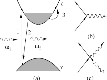
FIG. 1.: (a) Schematic representation of RRS in the direct gap two band model of electron doped GaAs nanostructure. $\omega_{i}$ and $\omega_{f}$ are the initial and final frequencies of the external photons. Steps 1, 2 and 3 are described in the text (RRS involves steps 1 and 2 only). (b) and (c) are the Feynman diagrams of the electron-photon scattering process described by $\mathbf{p}\it\cdot\mathbf{A}\it$ and $\mathbf{A}\it\cdot\mathbf{A}\it$ terms respectively in the interacting Hamiltonian, $H_{I}$. Solid and wavy lines represent the electron and photon Green’s functions respectively.

 

FIG. 2.: Diagrammatic representation of the conduction band irreducible response function, $\Pi^{\rm RPA}_{0}(\mathbf{q}\it,\omega)$ and reducible response function, $\Pi(\mathbf{q}\it,\omega)$, in the standard random phase approximation. $V_{c}(\mathbf{q}\it)$ is the Coulomb interaction.

 

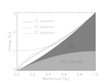
FIG. 3.: Typical momentum-energy dispersion of the single particle excitation continuum (shaded region) and the collective charge density excitations (plasmons) of one, two, and three dimensional electron systems (calculated within RPA).

 

 

 

FIG. 4.: Dynamical structure factor obtained by the standard (nonresonant) RPA calculation at zero temperature for (a) one, (b) two, and (c) three dimensional electron systems ignoring valence band effects. Solid lines are the calculated spectra in the long wavelength limit (small momentum transfer, $|\mathbf{q}\it|=\rm{0.1}\it k_{F}$) and dashed lines are for the large momentum transfer ($|\mathbf{q}\it|=\rm{0.7}\it k_{F}$ in (a) and (b), and $|\mathbf{q}\it|=\rm{0.4}\it k_{F}$ in (c)) calculations. The electron densities used in the calculation is $6.5\times 10^{5}$ cm^-1, $3.2\times 10^{11}$ cm^-2, and $1.8\times 10^{17}$ cm^-3 for one, two, and three dimensional systems respectively. Finite impurity scattering ($\gamma=10^{-3}E_{F}$) has been included to broaden the peaks. The ripple in (b) and (c) is of numerical origin.

 

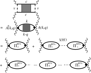
FIG. 5.: Diagrammatic representation of the resonant Raman scattering response function including the valence band electrons in the RPA calculation. Different kinds of irreducible response functions are defined and explained in Eqs. (17)-(19) and the matrix element, $A(\mathbf{k}\it,\mathbf{q}\it)$, is defined in Eq. (15).

 

 

 

FIG. 6.: Dynamical structure factor in the resonant RPA calculation for (a) one, (b) two, and (c) three dimensional electron systems incorporating the valence band electrons. We choose the resonance broadening factor, $\lambda$, to be $0.02E_{F}$, and finite impurity scattering factor, $\gamma$, to be 0.05 $E_{F}$ in order to have agreement with the experimental data (the impurity broadening is still rather small since $\gamma/E_{F}=1/20$). Other system parameters are the same as used in Fig. 4.

 

FIG. 7.: Ratio of the resonant Raman scattering spectral weight (CDE to SPE) as a function of the resonance energy, $E_{\omega}$, in one, two, and three dimensional systems. Off-resonance, $|E_{\omega}|\geq 0.2$, CDE always dominates SPE in the spectra, but near resonance, $|E_{\omega}|<0.2$, the SPE weight could even be stronger than the CDE weight. All system parameters are the same as used in Fig. 6.

REFERENCES

- [1] A. R. Goi, A. Pinczuk, J. S. Weiner, J. M. Calleja, B. S. Dennis, L. N. Pfeiffer, and K. W. West, Phys. Rev. Lett. 67, 3298 (1991).
- [2] C. Schller, G. Biese, K. Keller, C. Steinebach, and D. Heitmann, Phys. Rev. B 54, R17304 (1996).
- [3] B. Jusserand, M. N. Vijayaraghavan, F. Laruelle, A. Cavanna, and B. Etienne, Phys. Rev. Lett. 85, 5400 (2000).
- [4] Pinczuk, A, Brillson, L., and Burstein, E., Phys . Rev. Lett. 27, 317 (1971).
- [5] A. Pinczuk, J. P. Valladares, D. Heiman, A. C. Gossard, J. H. English, C. W. Tu, L. Pfeiffer, and K. West, Phys. Rev. Lett. 61, 2701 (1988).
- [6] A. Pinczuk, S. Schmitt-Rink, G. Danan, J. P. Valladares, L. N. Pfeiffer, and K. W. West, Phys. Rev. Lett. 63, 1633 (1989).
- [7] D. Gammon, B. V. Shanabrook, J. C. Ryan, and D. S. Katzer, Phys. Rev. B 41, 12311 (1990); M. Berz, J. F. Walker, P. von Allmen, E. F. Steigmeier, and F. K. Reinhart, Phys. Rev. B 42, 11957 (1990).
- [8] A. Pinczuk, B. S. Dennis, L. N. Pfeiffer, and K. West, Phys. Rev. Lett. 70, 3983 (1993).
- [9] D. Gammon, B. V. Shanabrook, J. C. Ryan, and D. S. Katzer, Phys. Rev. Lett. 68, 1884 (1992); R. Decca, A. Pinczuk, S. Das Sarma, B. S. Dennis, L. N. Pfeiffer, and K. W. West, Phys. Rev. Lett. 72, 1506(1996).
- [10] A. Schmeller, A. R. Goi, A. Pinczuk, J. S. Weiner, J. M. Calleja, B. S. Dennis, L. N. Pfeiffer, and K. West, Phys. Rev. B 49, 14778 (1994).
- [11] R. Strenz, U. Bockelmann, F. Hirler, G. Abstreiter, G. Bhm, and G. Weimam, Phys. Rev. Lett. 73, 3022 (1994).
- [12] S. Das Sarma and D. W. Wang, Phys. Rev. Lett. 83, 816 (1999).
- [13] M. Sassetti and B. Kramer, Phys. Rev. Lett. 80, 1485 (1998).
- [14] D. W. Wang, A. J. Millis, and S. Das Sarma, Phys. Rev. Lett. 85, 4570 (2000); and unpublished.
- [15] D. W. Wang and S. Das Sarma, cond-mat/0101061 (2001).
- [16] J. K. Jain, and P. B. Allen, Phys. Rev. Lett. 54, 947 (1985); J. K. Jain, and P. B. Allen, Phys. Rev. Lett. 54, 2437 (1985); S. Das Sarma and E. H. Hwang, Phys. Rev. Lett. 81, 4216 (1998).
- [17] J. K. Jain, and S. Das Sarma, Phys. Rev. B 36, 5949 (1987); J. K. Jain, and S. Das Sarma, Surf. Sci. 196, 466 (1988).
- [18] S. Das Sarma, Elementary Excitations in Low-Dimensional Semiconductor Structures. p. 499 in Light scattering in Semiconductor Structures and Superlattices, edited by Lockwood, D. J. and Young, J. F. (Plenum, New York, 1991).
- [19] A. Pinczuk, B. S. Dennis, L. N. Pfeiffer, and K. W. West, Philosophical Magazine B 70, 429 (1994) and references therein.
- [20] D. Pines, and P. Nozieres, The Theory of Quantum Liquids (Benjamin, New York, 1966).
- [21] A. L. Fetter and J. D. Walecka, Quantum Theory of Many-particle Systems, (McGraw-Hill, San Francisco, 1971).
- [22] I. K. Marmorkos and S. Das Sarma, Phys. Rev. B 45, 13396 (1992).
- [23] P. A. Wolff, Phys. Rev. 171, 436 (1968); F. A. Blum, Phys. Rev. B 1, 1125 (1970).
- [24] S. Das Sarma and E. H. Hwang, Phys. Rev. B 54, 1936 (1996).
- [25] H. J. Schulz, Phys. Rev. Lett. 71, 1864 (1993).
- [26] For a review of 1D Luttinger liquids, see for example, J. Voit, Rep. Prog. Phys., 58, 977 (1995).
- [27] M. V. Klein, Electronic Raman Scattering. p. 147 in Light Scattering in Solids, edited by Cardona, M. (Springer-Verlag, New York, 1975).
- [28] E. Burstein, A. Pinczuk, and D. L. Millis, Surf. Sci. 98, 451 (1980).
- [29] A. Pinczuk, and G. Abstreiter, Spectroscopy of Free Carrier Excitations in Semi-Conductor Quantum Wells. p. 153 in Light Scattering in Solids V, edited by Cardona, M. and Gntherodt, G. (Springer-Verlag, New York, 1989).
- [30] S. Das Sarma and W. Y. Lai, Phys. Rev. B 32, 1401 (1985); B. Yu-Kuang Hu and S. Das Sarma, Phys. Rev. B 48, 5469 (1992).
- [31] J. J. Sakurai, Advanced Quantum Mechanics (Addison-Wesley, Redwood, 1984).
- [32] P. A. Wolff, Phys. Rev. Lett. 16, 225 (1966).
- [33] Q. P. Li, and S. Das Sarma, Phys. Rev. B 43, 11768 (1991).
- [34] P. I. Tamborenea, and S. Das Sarma, Phys. Rev. B 49, 16821 (1994).
- [35] I. E. Dzyaloshinkii and A. I. Larkin, Sov. Phys.-JETP 38, 202 (1974); J. Slyom, Adv. Phys., 28, 201 (1979).