[

Time-resolved spectroscopy of multi-excitonic decay in an InAs quantum dot

Abstract

The multi-excitonic decay process in a single InAs quantum dot is studied through high-resolution time-resolved spectroscopy. A cascaded emission sequence involving three spectral lines is seen that is described well over a wide range of pump powers by a simple model. The measured biexcitonic decay rate is about 1.5 times the single-exciton decay rate. This ratio suggests the presence of selection rules, as well as a significant effect of the Coulomb interaction on the biexcitonic wavefunction.

]

Electrostatic interactions play an important role in the energy structures of semiconductor quantum dots[3] containing multiple particles. Although these interactions are usually treated as small perturbations to the single-particle wavefunctions, they lead to significant energy shifts that have been measured.[4, 5, 6, 7] These effects offer possibilities for new quantum-optical devices such as single-photon sources,[8, 9] entangled photon sources,[10] and perhaps even a method to implement quantum logic.[11]

Single-exciton and multi-exciton states, generated by adding electron-hole pairs to a dot, are of special interest for optical experiments. They are ideally the only states that can be generated through resonant optical excitation of quantum-dot transitions, and they also appear to be the states most commonly seen in above-band excitation experiments. Identification of individual multi-excitonic emission lines was originally based on the dependence of the emission intensity on the laser excitation power. More recently, time-resolved measurements on single quantum dots have become possible,[12, 13, 14] and measurements of biexcitonic emission from single CdSe dots[15] and multi-excitonic emission from ensembles of CdSe and CuCl nanocrystals[16, 17] and single InAs dots[18] have been performed.

Here, we report high-resolution time-resolved measurements on a single InAs dot using a streak camera system. After identifying the single-exciton and multi-exciton emission lines, we measure their decay rates, and find that the ratio of the one-exciton and biexciton decay rates is about 1:1.5. This is closer to the ratio expected for independent exciton recombination (1:2) than ratios reported for other material systems. [15, 16, 17] This result suggests the presence of strong selection rules, as well as a significant effect of the Coulomb interaction on the wavefunctions of multi-exciton states. We finally show that the data may be fit well over a wide range of excitation powers using a simple model.

The InAs self-assembled quantum dots used in this study were grown by molecular beam epitaxy at a high temperature ($520^{\circ}{\rm C}$) to increase alloying between the InAs and the surrounding GaAs, yielding ground-state emission wavelengths in the range of 860-$900\,{\rm nm}$. The potential wells of the dots are thus rather shallow, and even the first excited states are close in energy to the wetting layer. The dots are approximately $30\,{\rm nm}$ wide, with a density of about $11\,\mu{\rm m}^{-2}$. Small mesas (200 or $400\,{\rm nm}$ diameter) were then fabricated by electron-beam lithography and plasma etching to isolate single dots. Mesas containing exactly one dot were identified through their optical emission spectra. The spectra shown in Fig. 1(a),(b) were obtained from two mesas (mesas A and B, respectively) that have similar emission patterns, under continuous-wave (CW) excitation above the GaAs bandgap ($655\,{\rm nm}$ excitation wavelength). We identify the lines labeled 1 and 2 as one-exciton and two-exciton emission, since their dependences on excitation power are linear and quadratic, respectively, and since photon correlation measurements have confirmed their link. The lines labeled $1^{\prime}$ and $1^{\prime\prime}$ have linear pump power dependence, but are identified as charged-state[19] emission, since they disappear under excitation resonant with a higher energy level in the dot, as is seen in Fig. 1(c).

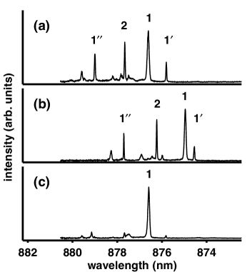
FIG. 1.: Emission spectra of (a) mesa A and (b) mesa B under CW, above-band ($655\,{\rm nm}$) excitation, and (c) of mesa A under CW, resonant ($858\,{\rm nm}$) excitation. Lines 1 and 2 are one- and two-exciton emission, respectively, while lines $1^{\prime}$ and $1^{\prime\prime}$ are believed to be charged-exciton emission.

Single mesas at a temperature of $5\,{\rm K}$ were excited from a steep angle ($54^{\circ}$ from normal) by $3\,{\rm ps}$ pulses every $13\,{\rm ns}$ from a Ti-sapphire laser, focused down to an $18\,\mu{\rm m}$ effective spot diameter. The resulting emission was collected by an ${\rm NA}=0.5$ aspheric lens, spectrally filtered to reject scattered laser light, and imaged onto a removable pinhole, which selected emission from a $5\,\mu{\rm m}$ region of the sample. The emission was then sent to an alignment camera, a spectrometer, or a streak camera system, which included a monochrometer that determined both the spectral ($0.13\,{\rm nm}$) and temporal ($25\,{\rm ps}$) resolutions. The streak camera recorded the emission following the excitation pulses, averaged over about 5 minutes ($2.3\times 10^{10}$ pulses). The resulting images were corrected for dark current, non-uniform sensitivity, and a small number of cosmic ray events.

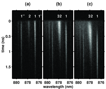
FIG. 2.: Streak camera images of emission from mesa A under pulsed, $708\,{\rm nm}$ laser excitation with powers (a) 27 $\mu{\rm W}$, (b) 108 $\mu{\rm W}$, and (c) 432 $\mu{\rm W}$. For larger powers, a cascaded emission is seen, with the multi-excitonic emission (lines 2, 3) occurring first, followed by one-exciton emission (line 1).

Images obtained under above-band ($708\,{\rm nm}$), pulsed laser excitation of mesa A with three different excitation powers are shown in Fig. 2. The observed emission lines are labeled as in Fig. 1. Figure 2(a) shows that under weak excitation ($27\,\mu{\rm W}$), the single-exciton line (line 1) appears less than $0.1\,{\rm ns}$ after the excitation pulse, and then decays exponentially. We attribute the small initial delay to the time required for electrons and holes generated by the excitation pulse to be captured by the dot. However, when the excitation power is increased to $108\,\mu{\rm W}$, Fig. 2(b) shows that line 1 reaches its maximum only after a delay of about $0.5\,{\rm ns}$. Most of the emission immediately after the excitation pulse now comes from the multi-exciton lines 2 and 3. In this case, the laser pulse initially creates several electron-hole pairs, and some time is required before the population in the dot reduces to one electron-hole pair, after which one-exciton emission occurs. Under strong excitation ($432\,\mu{\rm W}$), one can see from Fig. 2(c) that the delay in the one-exciton emission is even longer, and a delay also appears for lines 2 and 3. Only the broadband emission in the vicinity of the multi-exciton lines is seen to appear immediately after the excitation pulse.

The multi-excitonic decay process may be described by the following rate equation:

$$\frac{d}{dt}P_{n}(t)=\gamma_{n+1}P_{n+1}(t)-\gamma_{n}P_{n}(t)\,,\\$$ (1)

where $P_{n}(t)$ is the probability that $n$ electron-hole pairs exist in the dot at time $t$, and $\gamma_{n}$ is the decay rate of the $n$-pair state. The creation of charged dot states is not considered here. Instead, we apply this model only to neutral-dot outcomes following an excitation pulse by excluding emission lines $1^{\prime}$ and $1^{\prime\prime}$ from the analysis, and noting that radiative decay beginning with a neutral state cannot generate charged states. The form of $\gamma_{n}$ depends strongly on the nature of the states of the system. For an uncorrelated system with no recombination selection rules, one might expect $\gamma_{n}=n^{2}\gamma_{1}$. For a dot much smaller than the exciton Bohr radius, the Coulomb interaction has little effect on the wavefunctions of multi-exciton states, and due to selection rules one expects approximately independent recombination, $\gamma_{n}=n\gamma_{1}$. For a larger dot, it has been predicted that the Coulomb interaction produces a spatial separation between holes in multi-exciton states, so that, for example, the biexciton state resembles a molecule [15, 20]. In this case, one expects $\gamma_{n}<n\gamma_{1}$, and this has been observed for CdSe quantum dots.[15]

The decay rates $\gamma_{n}$ in Eq. 1 can be measured directly from the time-dependent intensities of the lines corresponding to $P_{n}(t)$, when $P_{n}(t)\gg P_{n+1}(t)$. To perform this measurement as accurately as possible, we tuned the excitation laser to a resonance at about $858\,{\rm nm}$, as in Fig. 1(c), creating electron-hole pairs directly inside the dot, which rapidly relax to a lowest-energy state. This way, the delayed capture of electrons and holes, which can alter the apparent decay rates, does not occur, as it could in the above-band excitation case. The excitation power (about $2\,{\rm mW}$) was chosen so that multi-exciton states were created with significant probability. The intensities of lines 1, 2, and 3 were calculated in a straightforward manner, by integrating the streak camera image over strips about $0.2\,{\rm nm}$ wide, defined to include all of the emission from each line. Lines 2 and 3 were not completely resolved, and the integration boundary was placed midway between them. A further concern for the multi-exciton lines 2 and 3 is that any weak background emission related to the one-exciton or charged-exciton states having a slower decay will cause significant distortion at large $t$, which is where we must measure the decay rates. With these cautions in mind, Fig. 3(a) shows the time-dependent intensities of lines 1, 2, and 3 under resonant excitation and a 60-minute integration, plotted on a semi-logarithmic scale. The slopes are estimated over the indicated regions by least-squares exponential fits. The time constants obtained are $0.479\,{\rm ns}$, $0.316\,{\rm ns}$, and $0.248\,{\rm ns}$, respectively. The one-exciton (line 1) lifetime seen here is close to the value of $0.47\,{\rm ns}$ we have measured with weaker excitation powers. We obtain $\gamma_{2}=1.52\gamma_{1}$, a result in between the small-dot limit ($\gamma_{2}=2\gamma_{1}$) and what has been reported for CdSe dots ($\gamma_{2}\approx\gamma_{1}$).[15] This is consistent with the presence of selection rules and a departure from the small-dot limit, due to the influence of the Coulomb interaction on the multi-exciton wavefunctions. Line 3 is likely due to emission from the 3-exciton state, since its wavelength relative to the one-exciton and biexciton lines is similar to what has been reported elsewhere for the 3-exciton line,[21] and this identification is made plausible here by its time dependence. With this assumption, we obtain $\gamma_{3}=1.93\gamma_{1}$.

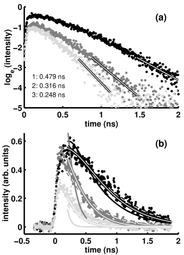
FIG. 3.: (a) Time-dependent intensities of lines 1 (black), 2 (dark gray), and 3 (light gray) from mesa A under pulsed, resonant ($858\,{\rm nm}$, $2\,{\rm mW}$) laser excitation. Exponential fits are applied after sufficient decay has occurred to estimate the decay times. (b) Time-dependent intensities under above-band ($708\,{\rm nm}$, $54\,\mu{\rm W}$) excitation, compared to three models: $\gamma_{n}=n\gamma_{1}$ (hollow lines), measured decay rates (hollow, dashed), and $\gamma_{n}=n^{2}\gamma_{1}$ (solid).

We now wish to model the multi-excitonic decay process under above-band excitation over a wide range of excitation powers, to show that the behavior of lines 1, 2, and 3 is consistent with a cascaded decay. We assume that photons from the laser excitation pulse are absorbed independently by the GaAs surrounding the dot to form electron-hole pairs, and that these pairs are then independently captured by the dot, so that the initial population of the dot follows a Poisson distribution with mean $\mu$. The dot then decays according to Eq. 1, and we assume that the observed intensity from the $n$-exciton state is $I_{n}=\gamma_{n}I_{0}P_{n}$, where $I_{0}$ includes the collection efficiency. We make this assumption for simplicity, though it does not take into account the presence of multiple emission lines for $n>2$. Fig. 3(b) shows the time-dependent intensities of lines 1, 2, and 3 under above-band ($708\,{\rm nm}$, $54\,{\rm mW}$) excitation, along with three models, each simultaneously fit to lines 1 and 2. The predicted 3-exciton behavior is also shown, in comparison to line 3.

In the first model (hollow lines), we assume independent recombination, $\gamma_{n}=n\gamma_{1}$. Although this assumption differs substantially from the measured rates, its simplicity is appealing. The resulting time-dependent probabilities have the simple form of a Poisson distribution with exponentially decaying mean:

$$P_{n}(t)=(\mu e^{-\gamma_{1}t})^{n}\exp(-\mu e^{-\gamma_{1}t})/n!\,,$$ (2)

where $\mu$ is again the mean initial exciton number. This model is also well suited to handle an additional complication noticeable in the data. For above-band excitation, a finite time is required for the dot to capture the excitons generated by the laser pulse, with some recombination occurring during this time. But since, in this model, the excitons are both generated and annihilated independently, a Poisson distribution always holds, and it is sufficient to wait until the capture process has finished ($0.2\,{\rm ns}$) to begin fitting the data to Eq. 2. In the second model (hollow, dashed lines), Eq. 1 is solved numerically, using the measured decay rates and assuming a Poisson distribution, beginning at $0.2\,{\rm ns}$. The rates $\gamma_{n}$ for $n>3$ had to be extrapolated from the trend seen for $n\leq 3$, but have little effect on the result for this excitation power. In the third model (thin solid lines), Eq. 1 is solved numerically assuming $\gamma_{n}=n^{2}\gamma_{1}$, as one would expect with no recombination selection rules. For all three models, only two fitting parameters are used, the initial mean number of excitons $\mu$, and the collection efficiency constant, $I_{0}$. From these two fitting parameters, all three curves (one-exciton, biexciton, 3-exciton) are obtained simultaneously. Two of these cascaded decay models, the model with independent exciton decay ($\gamma_{n}=n\gamma_{1}$) and the model using measured decay rates, fit the data reasonably well (mean squared errors $8.2\times 10^{-4}$ and $9.4\times 10^{-4}$, respectively). The other model ($\gamma_{n}=n^{2}\gamma_{1}$) fits the data poorly (mean squared error $4.4\times 10^{-3}$).

To demonstrate that lines 1, 2, and 3 are well described by a cascaded emission process, we fit the simplest model ($\gamma_{n}=n\gamma_{1}$) to the data for four different pump powers in Fig. 4. The value of $\gamma_{1}$ was fixed at $(0.47\,{\rm ns})^{-1}$, and the obtained values of the fitting parameters $I_{0}$ and $\mu$ are shown. The value of $\mu$ increases linearly with excitation power at first, and then begins to saturate. Ideally, $I_{0}$ should be the same for each streak camera image, but in our case, we had to fit it separately for each image due largely to spatial sample drift and streak-camera gain drift. The fit was performed to minimize the combined errors for lines 1 and 2. For all three lines, the simple model provides excellent agreement with the data in the weak, moderate, and strong-excitation cases, supporting the presence of a multi-excitonic decay sequence involving these lines.

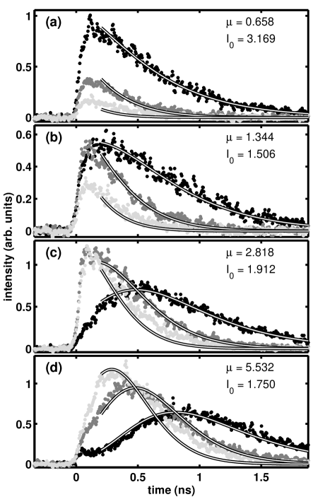
FIG. 4.: Time-dependent intensities of lines 1 (black), 2 (dark gray), and 3 (light gray) from mesa A under pulsed, $708{\rm nm}$ laser excitation with powers (a) 27 $\mu{\rm W}$, (b) 54 $\mu{\rm W}$, (c) 108 $\mu{\rm W}$, and (d) 432 $\mu{\rm W}$. Hollow lines show model fit results, and fit parameters are given at upper-right.

In summary, we have observed multi-excitonic decay spectra from a single quantum dot using a streak camera, providing high temporal resolution. We have measured the decay rates of several lines, and found that the biexciton decay rate is about 1.5 times the one-exciton decay rate, suggesting strong recombination selection rules and a significant influence of the Coulomb interaction on the multi-exciton wavefunctions. We then showed that, under above-band excitation, the time dependence of the emission lines is well described over a wide range of excitation powers by a simple model for cascaded emission.

Financial assistance for C. S. was provided by the National Science Foundation. Financial assistance for C. S. and M. P. was provided by Stanford University. G. S. S. is partially supported by ARO (D. Woolard).

REFERENCES

- [1] Also at Solid-State Photonics Laboratory, Stanford University, Stanford, CA.
- [2] Also at NTT Basic Research Laboratories, Atsugishi, Kanagawa, Japan.
- [3] D. Bimberg, M. Grundmann, and N. N. Ledentsov, Quantum Dot Heterostructures (John Wiley & Sons, Chichester, 1999).
- [4] A. Kuther, M. Bayer, A. Forchel, A. Gorbunov, V. B. Timofeev, F. Schäfer, and J. P. Reithmaier, Phys. Rev. B 58, R7508 (1998).
- [5] H. Kamada, H. Ando, J. Temmyo, and T. Tamamura, Phys. Rev. B 58, 16243 (1998).
- [6] L. Landin, M. S. Miller, M.-E. Pistol, C. E. Pryor, and L. Samuelson, Science 280, 262 (1998).
- [7] M. Bayer, O. Stern, P. Hawrylak, S. Fafard, and A. Forchel, Nature (London) 405, 923 (2000).
- [8] C. Santori, M. Pelton, G. Solomon, Y. Dale, and Y. Yamamoto, Phys. Rev. Lett. 86, 1502 (2001).
- [9] P. Michler, A. Kiraz, C. Becher, W. V. Schoenfeld, P. M. Petroff, L. Zhang, E. Hu, and A. Imamoğlu, Science 290, 2282 (2000).
- [10] O. Benson, C. Santori, M. Pelton, and Y. Yamamoto, Phys. Rev. Lett. 84, 2513 (2000).
- [11] F. Troiani, U. Hohenester, and E. Molinari, Phys. Rev. B 62, R2263 (2000).
- [12] Ph. Roussignol, W. Heller, A. Filoramo, and U. Bockelmann, Physica E 2, 588 (1998).
- [13] V. Zwiller, M.-E. Pistol, D. Hessman, R. Cederström, W. Seifert, and L. Samuelson, Phys. Rev. B 59, 5021 (1999).
- [14] D. V. Regelman, E. Dekel, D. Gershoni, W. V. Schoenfeld, and P. M. Petroff, Phys. Stat. Sol. (b), 224, 343 (2001).
- [15] G. Bacher, R. Weigand, J. Seufert, V. D. Kulakovskii, N. A. Gippius, A. Forchel, K. Leonardi, and D. Hommel, Phys. Rev. Lett. 83, 4417 (1999).
- [16] V. I. Klimov, A. A. Mikhailovsky, D. W. McBranch, C. A. Leatherdale, and M. G. Bawendi, Science 287, 1011 (2000).
- [17] M. Ikezawa and Y. Masumoto, Phys. Rev. B 53, 13694 (1996).
- [18] E. Dekel, D. V. Regelman, D. Gershoni, E. Ehrenfreund, W. V. Shoenfeld, and P. M. Petroff, Phys. Rev. B 62, 11038 (2000).
- [19] J. J. Finley, P. W. Fry, A. D. Ashmore, A. Lemaître, A. I. Tartakovskii, R. Oulton, D. J. Mowbray, M. S. Skolnick, M. Hopkinson, P. D. Buckle, and P. A. Maksym, Phys. Rev. B 63, 161305(R) (2001).
- [20] T. Takagahara, Phys. Rev. B 39, 10206 (1989).
- [21] A. Hartmann, Y. Ducommun, E. Kapon, U. Hohenester, and E. Molinari, Phys. Rev. Lett. 84, 5648 (2000).