Theory of the cold collision frequency shift in 1S–2S spectroscopy of Bose-Einstein-condensed and non-condensed hydrogen

Abstract

We show that a correct formulation of the cold collision frequency shift for two photon spectroscopy of Bose-condensed and cold non-Bose-condensed hydrogen is consistent with experimental data. Our treatment includes transport and inhomogeneity into the theory of a non-condensed gas, which causes substantial changes in the cold collision frequency shift for the ordinary thermal gas, as a result of the very high frequency (3.9kHz) of transverse trap mode. For the condensed gas, we find substantial corrections arise from the inclusion of quasiparticles, whose number is very large because of the very low frequency (10.2Hz) of the longitudinal trap mode. These two effects together account for the apparent absence of a “factor of two” between the two possibilities.

Our treatment considers only the Doppler-free measurements, but could be extended to Doppler-sensitive measurements. For Bose-condensed hydrogen, we predict a characteristic “foot” extending into higher detunings than can arise from the condensate alone, as a result of a correct treatment of the statistics of thermal quasiparticles.

1 Introduction

Bose-Einstein condensation of spin-polarized hydrogen, achieved in 1998 [4, 10, 9, 8, 3] as the culmination of a quarter of a century of development of cooling, trapping and spectroscopic techniques, still presents certain puzzling features. The most notable of these occurs in the spectroscopic method used to detect the condensate, based on two-photon excitation from the 1S to the 2S state of the hydrogen atom in the presence of a significant background density of hydrogen atoms—a density which of course becomes very large when the hydrogen Bose condenses. The cold collision frequency shift—a shift of the transition frequency proportional to the density of the gas—is measurable even when the gas is merely dense, but not Bose-condensed, and is very significant for the condensate. This has led to the use—suggested by Shlyapnikov (see reference [19] of [1])—of the cold collision frequency shift as a method of measuring the proportion of atoms which occur at a given density in the system of cold hydrogen atoms. The magnitude of the shift is expected to be twice as much for a given density for the non-condensed gas as for the Bose-condensate, as a result of the different coherence properties of the two systems. However, the frequency shifts observed have led the experimenters to the conclusion [4]:

…if we had assumed that the frequency shift in the condensate is only half as large as for a normal gas at the same density, as one would expect for a condensate in a single quantum state, the density extracted from the spectrum would be twice as large. This would imply that $N_{c}=6\times 10^{9}$ and yield an unreasonably high condensate fraction of 25%.

The apparent absence of the “factor of two” has led to the speculation that the hydrogen condensate is not in fact a true condensate, but is in some unexplained way incoherent, so that the behaviour is qualitatively similar to that of a non-condensed system, and Côté and Kharchenko [2] have given a more exotic explanation, based on droplet formation at the edge of the condensate. Our aim in this paper is to take the view that the hydrogen Bose-Einstein condensate has no exotic features, but to make a careful investigation of the physics of the two-photon excitation process used to probe the system, both when it is condensed and when it is non-condensed. In our view, the apparent absence of the “factor of two” implies that something is wrong with the theoretical treatment of the cold collision frequency shift in either the condensed system or the non-condensed system or possibly in both, as they have been so far formulated.

We have therefore reviewed the conventional theory in Sect.1, and have shown that for a non-condensed system it is assumed that the system is homogeneous. The treatment of the condensed system [8, 9] does not make this assumption, but requires the system to be a pure condensate. Neither of these requirements can be considered to be adequately met in current experiments, since the system is tightly trapped and relatively warm.

In Sect.2 we develop a theory of the cold collision frequency shift in inhomogeneous non-condensed systems, and show that in the published experiments [10, 4] the effect of the inhomogeneity will be very significant, and will tend to reduce the “factor of two” significantly. The main reason is quite straightforward. During the time of the exciting pulse the atoms move through a wide range of densities, and the coherence between the excited state and the ground state, necessary to produce the “factor of two”, cannot be established.

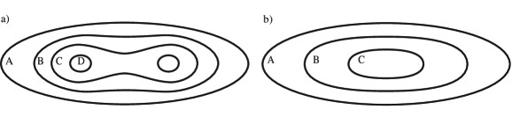
Figure 5: Illustration of the contours of excitation expected for a) The quasiparticle component and b) The condensate component. The letters A–D correspond to the frequencies $\Omega_{\rm A}$–$\Omega_{\rm D}$. Note that the highest frequency $\Omega_{\rm D}$ gives no condensate signal.

In Sect.3 we turn to the condensed system, and develop a formalism which uses a quasiparticle basis to give some linear partial differential equations for the excitation as a function of space and time. We use the very anisotropic aspect ratio of the hydrogen trap—about 400:1—to simplify our formalism to a relatively simple set of formulas from which quantitative predictions can be made. Our results confirm those of Killian [9] for a pure condensate, but also give results which are valid when a significant quasiparticle component is present. In essence we show that the quasiparticle component can be up to 20% of the apparent condensate occupations, and that the condensate and the quasiparticles give rise to independent and qualitatively different signals. For a given excitation frequency, the two signals are produced from different locations in the system—this can be seen as arising because there is not only a cold collision frequency shift  but as well a splitting which gives rise to two frequencies, the two components corresponding to the two signals. The situation is illustrated in Fig.5. In fact, at the highest detunings, the signal arises only from the quasiparticle component, and gives rise to a characteristic “foot” protruding into the high frequencies above an otherwise smooth spectrum, and indeed there is some experimental indication of such a feature—see Fig.6.

We conclude that if the our calculations for condensed and non-condensed experiments are taken into account that the data of [4] appear to be consistent with the following:

• The calculated value of the 1S-2S cross section.

• The condensate is coherent, and is accompanied by the appropriate distribution of quasiparticles for the measured temperature.

• The non-condensed system is incoherent, with $g_{2}=2$.

2 The cold collision frequency shift for a homogeneous system

In an inhomogeneous and possibly Bose condensed system, we consider the excitation by a coherent process. One photon excitation by a coherent microwave field is usual for an atomic clock, but in the case of a hydrogen Bose-Einstein condensate two-photon excitation is used to excite from the 1S to the 2S level. The exciting field is pulsed for a time very long compared to the transition frequency, but so short that only an infinitesimal proportion of the atoms are excited to the upper level.

2.1 Second-quantized Hamiltonian

For the case under consideration the second-quantized Hamiltonian can be written in the form

$$H = \int d^{3}{\bf x}\,\Bigg{\{}\psi^{\dagger}_{1}\left(T+V({\bf x})+\hbar\omega_{1}\right)\psi_{1}+\psi^{\dagger}_{2}\left(T+V({\bf x})+\hbar\omega_{2}\right)\psi_{2}$$

$$+{u\over 2}\psi^{\dagger}_{1}\psi^{\dagger}_{1}\psi_{1}\psi_{1}+{v}\psi^{\dagger}_{1}\psi^{\dagger}_{2}\psi_{1}\psi_{2}+{w\over 2}\psi^{\dagger}_{2}\psi^{\dagger}_{2}\psi_{2}\psi_{2}+gE({\bf x})\bigg{(}\psi^{\dagger}_{1}\psi_{2}e^{i\Omega t}+\psi^{\dagger}_{2}\psi_{1}e^{-i\Omega t}\bigg{)}\Bigg{\}}.$$

• The labels $1,2$ represent the 1S and 2S states of hydrogen, and $\hbar\omega_{1},\hbar\omega_{2}$ are 1S and 2S energy levels used in the experiment.

• The kinetic energy operator is $T=-\hbar^{2}\nabla^{2}/2m$

• This form assumes the trapping potentials have the same form $V({\bf x})$ for the 1S and the 2S states of hydrogen.

• Since the process being considered is a two-photon process, the driving term is proportional to the square of the laser field, which is assumed to have frequency $\Omega/4\pi$, and wavenumber ${\bf k}/2$, so that we can write the driving term using

  $$E({\bf x}) = E\big{(}1+\cos({\bf k}\cdot{\bf x})\big{)}.$$ (2)

  The spatially independent term gives the Doppler-free excitation, while the cosine term gives the Doppler-sensitive excitation. In the experiments both forms of excitation are used—however in this paper we shall treat mainly the Doppler-free case, for which we have been able to develop a relatively simple formalism.

• The interaction coefficients are given in terms of scattering lengths by

  $$u = {4\pi a_{\rm 1S-1S}\hbar^{2}/m}$$ (3)

  $$v = {4\pi a_{\rm 1S-2S}\hbar^{2}/m}$$ (4)

  $$w = {4\pi a_{\rm 2S-2S}\hbar^{2}/m}$$ (5)

  The scattering lengths have been calculated in [7, 6] to be

  $$a_{\rm 1S-1S} = \phantom{-}0.0648{\rm nm}$$ (6)

  $$a_{\rm 1S-2S} = -2.3{\rm nm},$$ (7)

  and the experimental value (calculated assuming that the theory of the cold collision frequency shift in a non-condensed trapped system is the same as that of a homogeneous trapped system)

  $$a_{\rm 1S-2S} = -1.4\pm 0.3{\rm nm}.$$ (8)

  is reported in [10].

• The coefficient $w$ will be set equal to zero, since its effect is in practice negligible with the densities of 2S atoms appropriate for the experiment.

2.2 Background

The approach used by Killian [9, 8] considers an initial many-body wavefunction composed as a symmetrized product of one-body wavefunctions $|1S\rangle$. The result of the laser excitation is to rotate the spin wavefunction slightly into the 2S subspace, so the one-body wavefunction is transformed

$$|1S\rangle\to t|1S\rangle+r|2S\rangle,$$ (9)

with $|t|^{2}+|r|^{2}=1$, and $r\ll 1$. In field theoretic language (in the Heisenberg picture) the initial state is described by field operators $\psi_{1}({\bf x})$, $\psi_{2}({\bf x})$ with $\langle\psi^{\dagger}_{2}({\bf x})\psi_{2}({\bf x})\rangle=0$, and these transform to

$$\psi_{1}({\bf x}) \to \phantom{-}t\psi_{1}({\bf x})+r\psi_{2}({\bf x})$$ (10)

$$\psi_{2}({\bf x}) \to -r\psi_{1}({\bf x})+t\psi_{2}({\bf x}).$$ (11)

and the population densities $n_{i}({\bf x})=\langle\psi^{\dagger}_{i}({\bf x})\psi_{i}({\bf x})\rangle$ transform as

$$n_{1}({\bf x})\to n_{1}({\bf x})-\delta n({\bf x}) = |t|^{2}n_{1}({\bf x}),$$ (12)

$$n_{2}({\bf x})\to\delta n({\bf x})\,\,\,\,\qquad\quad = |r|^{2}n_{1}({\bf x}).$$ (13)

The mean energy after this process is given by the sum of kinetic, potential and self energy terms. Since the trapping potentials for the two states are assumed the same, there is no change of trapping energy, and if the excitation is not strongly dependent on space there is no change in the kinetic energy term. Under these conditions the main energy change is given by the interaction energy, which changes by an average amount

$$\left({u\over 2}\left(|t|^{4}-1\right)+v|t|^{2}|r|^{2}\right)\langle\psi_{1}^{\dagger}({\bf x})\psi^{\dagger}_{1}({\bf x})\psi_{1}({\bf x})\psi_{1}({\bf x})\rangle \approx g_{2}({\bf x},{\bf x})(v-u)n_{1}({\bf x})\delta n({\bf x}).$$ (14)

Here we have used the spatial density correlation function

$$g_{2}({\bf x},{\bf x}^{\prime}) = {\langle\psi_{1}^{\dagger}({\bf x})\psi^{\dagger}_{1}({\bf x}^{\prime})\psi_{1}({\bf x})\psi_{1}({\bf x}^{\prime})\rangle\over n_{1}({\bf x})n_{1}({\bf x}^{\prime})}.$$ (15)

If the initial quantum state is noncondensed, it can be written in terms of a set of orthonormal one particle wavefunctions $\phi_{r}({\bf x)}$ with occupations $N_{r}$ which are either 0 or 1, so that

$$n_{1}({\bf x}) = \sum_{r}|\phi_{r}({\bf x)}|^{2}N_{r},$$ (16)

$$g_{2}({\bf x},{\bf x})n_{1}({\bf x})^{2} = 2\sum_{{r,s}\atop r\neq s}|\phi_{r}({\bf x)}|^{2}|\phi_{s}({\bf x)}|^{2}N_{r}N_{s}$$ (17)

$$\approx 2n_{1}({\bf x})^{2},$$ (18)

where the approximate final result is valid provided the occupation is spread over very many modes, so that the missing term with $r=s$ is negligible. Thus we find in this case $g_{2}({\bf x},{\bf x})\to 2$. This result is also obviously true for an ensemble of noncondensed quantum states, such as a thermal noncondensed state.

If the state is condensed in the sense that only the quantum state $r=r_{0}$ is occupied, and $N_{r_{0}}\gg 1$ , then the same calculation leads to $g_{2}({\bf x},{\bf x})\to 1$, so that the energy shift is only half of the value expected from a noncondensed state—the “factor of two” thus does appear when the trapping and kinetic parts of the Hamiltonian can be neglected.

2.2.1 Issues for a realistic condensate

There are three main issues which need to be addressed

• The energy shift is proportional to $n_{1}({\bf x})$, and is sufficiently large in practice for it to be used as a spectroscopic method of measuring the density profile of a very cold and possibly condensed cloud of hydrogen atoms. Thus the amplitude $t$ for transition to the 2S state is of necessity spatially dependent. This issue has been addressed in [9, 8] for the case of a pure condensate, but it has been assumed that the results of the homogeneous noncondensed system are applicable to the inhomogeneous non-condensed case which occurs in the experiments. A full consideration of the effects of inhomogeneity for a noncondensed system or a partially condensed system has not been made.

• The temperature of the condensed system is relatively high, so that occupation of the lowest quasiparticle levels is significant. We showed previously [5] that this could be up to 20% of the apparent condensate population, and that the effective $g_{2}({\bf x},{\bf x})$ in such a situation is spatially dependent, varying from a little more than 1 to somewhat larger than 2, depending on the position in the condensate. Under these conditions the simple argument given above cannot be justified.

• The estimate of the energy shift (14) uses an average energy. However, at a given position in space, this could be the result of an average of different eigenvalues, and it would be these eigenvalues which were selected spectroscopically, not their average, leading to a given resonant frequency corresponding to different densities of the gas.

3 Cold collision frequency shift for an inhomogeneous non-condensed system

As noted above, the “factor of 2” has been derived only for homogeneous systems, and in the experiments [9, 8] homogeneity is not satisfied. One need only note:

The radial trap frequency is $$\approx 3.9\mbox{kHz}$$

The axial trap frequency is $$\approx 10\mbox{Hz}$$

The laser pulse length is $$\approx 500\mu\rm{s}\approx 2\mbox{ radial trap periods.}$$

Thus, during the period of the excitation it will be possible for a significant number of atoms to experience a wide range of values of the vapour density, and a treatment must be devised which includes the full dynamics of transport in the tightly trapped cloud. We will show that a combined transport-excitation equation in 3 position plus 3 momentum variables can be derived.

3.1 Equations of motion

From the Hamiltonian (2.1) the Heisenberg equations of motion for the field operators are (in the Doppler-free case)

$$i\hbar\dot{\psi}_{1} = [\hbar\omega_{1}+H({\bf x})]\psi_{1}+u\psi_{1}^{\dagger}\psi_{1}\psi_{1}+v\psi_{2}^{\dagger}\psi_{1}\psi_{2}+gEe^{i\Omega t}\psi_{2}$$ (19)

$$i\hbar\dot{\psi}_{2} = [\hbar\omega_{2}+H({\bf x})]\psi_{2}+v\psi_{1}^{\dagger}\psi_{1}\psi_{2}+gEe^{-i\Omega t}\psi_{1},$$ (20)

in which

$$H({\bf x}) \equiv -{\hbar^{2}\nabla^{2}\over 2m}+V({\bf x}).$$ (21)

We suppose that the occupation of the 1S level is always very much greater than that of the 2S level, and all of this occupation induced by the application of the coherent driving field $E$. This means that we can neglect entirely the last two terms in (19), so that $\psi_{1}({\bf x},t)$ can be regarded as a known time-dependent operator.

We now define Wigner amplitudes

$$f({\bf p},{\bf x}) = {1\over h^{3}}\int d^{3}{\bf y}\langle\psi_{1}^{\dagger}({\bf x}-{\bf y}/2)\psi_{2}({\bf x}+{\bf y}/2)\rangle e^{-i{\bf p}\cdot{\bf y}/\hbar}$$ (22)

$$n({\bf p},{\bf x}) = {1\over h^{3}}\int d^{3}{\bf y}\langle\psi_{1}^{\dagger}({\bf x}-{\bf y}/2)\psi_{1}({\bf x}+{\bf y}/2)\rangle e^{-i{\bf p}\cdot{\bf y}/\hbar}$$ (23)

We will also use the momentum integrated quantities

$$N({\bf x}) = \int d^{3}{\bf p}\,n({\bf p},{\bf x})\equiv\ \langle\psi_{1}^{\dagger}({\bf x})\psi_{1}({\bf x})\rangle$$ (24)

$$F({\bf x}) = \int d^{3}{\bf p}\,f({\bf p},{\bf x})\equiv\ \langle\psi_{1}^{\dagger}({\bf x})\psi_{2}({\bf x})\rangle$$ (25)

which will characterize the system sufficiently for our purposes. We can now derive equations of motion using

• Hartree-Fock factorization in the form (for example)

  $$\langle\psi_{1}^{\dagger}({\bf z}).\psi_{1}^{\dagger}({\bf z}^{\prime})\psi_{1}({\bf z}^{\prime})\psi_{2}({\bf z}^{\prime})\rangle$$

  $$\qquad\qquad=\langle\psi_{1}^{\dagger}({\bf z})\psi_{1}({\bf z}^{\prime})\rangle\langle\psi_{1}^{\dagger}({\bf z}^{\prime})\psi_{2}({\bf z}^{\prime})\rangle+\langle\psi_{1}^{\dagger}({\bf z})\psi_{2}({\bf z}^{\prime})\rangle\langle\psi_{1}^{\dagger}({\bf z}^{\prime})\psi_{1}({\bf z}^{\prime})\rangle,$$ (26)

  with ${\bf z}\equiv{\bf x}-{\bf y}/2$ and ${\bf z}^{\prime}\equiv{\bf x}+{\bf y}/2$.

• Since the terms $\langle\psi_{1}^{\dagger}({\bf z})\psi_{1}({\bf z}^{\prime})\rangle$, $\langle\psi_{1}^{\dagger}({\bf z})\psi_{2}({\bf z}^{\prime})\rangle$ can only be nonzero for very small ${\bf y}={\bf z}-{\bf z}^{\prime}$, we also make the approximations of the form

  $$\langle\psi_{1}^{\dagger}({\bf z}^{\prime})\psi_{1}({\bf z}^{\prime})\rangle \equiv n({\bf z}^{\prime})\approx n({\bf x})+{\bf y}\cdot\nabla n({\bf x})/2.$$ (27)

• We can then use the standard Wigner function methods to get the equation of motion

  $$i\hbar{\partial f({\bf p},{\bf x})\over\partial t} = \hbar(\omega_{2}-\omega_{1})f({\bf p},{\bf x})+gEe^{-i\Omega t}n({\bf p},{\bf x})$$ (28)

  $$+i\hbar\left\{-({\bf p}/m)\cdot\nabla_{x}+\nabla V({\bf x})\cdot\nabla_{p}\right\}f({\bf p},{\bf x})$$

  $$-(2u-v)N({\bf x})f({\bf p},{\bf x})+vF({\bf x})n({\bf p},{\bf x})$$

  $$+i\hbar\left(u+{v\over 2}\right)\nabla N({\bf x})\cdot\nabla_{p}f({\bf p},{\bf x})+i\hbar{v\over 2}\nabla F({\bf x})\cdot\nabla_{p}n({\bf p},{\bf x}).$$

3.1.1 The measured signal

The measured signal is the total number of atoms excited to the 2S level, that is

$$S(\Omega) = \int d^{3}{\bf x}\langle\psi_{2}^{\dagger}({\bf x})\psi_{2}({\bf x})\rangle.$$ (29)

We can use an ansatz

$$\psi_{2}({\bf x}) \approx \int d^{3}{\bf y}\,r({\bf x},{\bf y})\psi_{1}({\bf y})$$ (30)

to express the linearity of the process, in the sense of (10,11), and then we can write

$$\bar{f}({\bf y},{\bf x}) \equiv \langle\psi_{1}^{\dagger}({\bf y})\psi_{2}({\bf x})\rangle\approx\int d^{3}{\bf y}^{\prime}\,r({\bf x},{\bf y}^{\prime})\langle\psi_{1}^{\dagger}({\bf y})\psi_{1}({\bf y}^{\prime})\rangle.$$ (31)

It is reasonable to approximate the correlation function on the right hand side of this equation by a locally thermal form

$$\langle\psi_{1}^{\dagger}({\bf y})\psi_{1}({\bf y}^{\prime})\rangle \approx N\left({{\bf y}+{\bf y}^{\prime}\over 2}\right)\exp\left(-{({\bf y}-{\bf y}^{\prime})^{2}\over 2L^{2}}\right),$$ (32)

in which

$$L \equiv \hbar/\sqrt{2\pi{mkT}}.$$ (33)

The length $L$ is sufficiently short in a thermal situation to treat the correlation function as being essentially local in (30,31), and thus write

$$\bar{f}({\bf y},{\bf x}) \approx (\sqrt{2\pi}L)^{3}N({\bf y})r({\bf x},{\bf y}),$$ (34)

and using this we can then similarly derive

$$S(\Omega) \approx \int d^{3}{\bf x}\int d^{3}{\bf y}{|\bar{f}({\bf y},{\bf x})|^{2}\over(\sqrt{2\pi}L)^{3}N({\bf y})}\quad.$$ (35)

3.2 The homogeneous case

Suppose now that $V({\bf x})=0$, and $n({\bf p},{\bf x})\equiv n_{\rm hom}({\bf p})$ is independent of ${\bf x}$. There is then a solution of (28) with $f({\bf p},{\bf x})\propto n({\bf p})$, also independent of ${\bf x}$ and the corresponding equation of motion can be integrated over ${\bf p}$ to give

$$i\hbar{\partial F\over\partial t} = \{\hbar(\omega_{2}-\omega_{1})-2(u-v)N\}F+gENe^{-i\Omega t}$$ (36)

Thus in this case we find that

$$\bar{f}({\bf y},{\bf x}) \to F\exp\left(-{({\bf y}-{\bf x})^{2}\over 2L^{2}}\right)$$ (37)

and

$$S(\Omega) \to {|F|^{2}V\over{2\sqrt{2}}N}$$ (38)

where $V$ is the volume of the homogeneous system being observed. We can easily solve the equations (36) to get

$$S(\Omega) = {N_{\rm tot}(gE)^{2}\over{2\sqrt{2}}\hbar^{2}}{\sin^{2}\left\{\left(\Omega-\Delta\right)T/2\right\}\over\left\{\left(\Omega-\Delta\right)/2\right\}^{2}}\$$ (39)

$$\to {N_{\rm tot}(gE)^{2}\over{2\sqrt{2}}\hbar^{2}}2\pi T\,\delta(\Omega-\Delta).$$ (40)

$$\mbox{where }\Delta = \omega_{2}-\omega_{1}-{2(u-v)N\over\hbar}$$ (41)

This confirms the result of (14) with $g_{2}=2$.

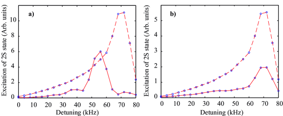
Figure 1: Excitation as a function of laser detuning. In all cases the laser is turned on for a time $T=500\mu{\rm s}$. The solid curves are solutions of the equations (28), the dashed curves omit the “streaming terms” on the second line of (28). a) $\omega_{r}=3.9{\rm kHz}$ ; b) $\omega_{r}=780{\rm Hz}$.

3.3 One dimensional solutions of the equations of motion

The equations (28) form a six-dimensional set, which are quite formidable to solve numerically, so to get an idea of their effect, we have done one-dimensional solutions, with trap frequency $\omega_{r}$. The results are presented in Fig.1 The solutions of the equations obtained by omitting the “streaming term” on the second line of (28)—corresponding to the result (14)—are given in the dashed curves. It can be seen that for the trap frequency frequency of $\omega_{r}=2\pi\times 3.9{\rm kHz}$ , as used in the experiments, the excitation curve is very strongly affected, but for the frequency $\omega^{\prime}_{r}=\omega_{r}/5=2\pi\times 780{\rm Hz}$, one fifth of that frequency, although there is a small quantitative difference in excitation, the shape is essentially unchanged. These should be compared with the excitation time $T=500\mu{\rm s}$ for which $\omega_{r}T/2\pi=1.95$, while $\omega^{\prime}_{r}T/2\pi=0.39$. The conclusions we can draw from these one dimensional simulations are limited to the observation that the peak of the solid curve in Fig.1 is shifted from the position which would be expected if one used the homogeneous system formulation of Sect. 2.2. The shift of the peak is such that one would see an apparent “factor of about $1.57$”, rather than the “factor of 2”, and this would indicate that the true 1S–2S scattering length should be larger than the experiments have actually measured. We are reluctant to treat the value 1.57 as anything other than a qualitative result, but it seems that this would suggest that it might be wiser to use the theoretical value (7) in analysing the condensate data rather than the apparent measured value (8).

4 Cold collision frequency shift for an inhomogeneous condensed or partially condensed system

The treatment in the presence of a condensate takes a completely different form from the full thermalized case. As before, the equations cannot be solved exactly, but approximate equations of motion which incorporate the features of the quasiparticle spectrum, as investigated in [5], can be developed as follows.

4.1 Approximate equation of motion

The equations of motion and assumptions used in Sect.3.1 are valid in this case as well, but the Wigner function methodology is not appropriate, since its use depends on hartree-Fock factorization.

4.1.1 Quasiparticle expansions

As before, we suppose that the occupation of the 1S level is always very much greater than that of the 2S level, so that $\psi_{1}({\bf x},t)$ can be regarded as a known time-dependent operator. However, in this case we represent the time-dependent solution for $\psi_{1}({\bf x},t)$ by a quasiparticle expansion of the form

$$\psi_{1}({\bf x},t) = a_{0}(t)\Bigg{(}{\xi({\bf x})\over\sqrt{n_{0}}}+{1\over\sqrt{n_{0}}}\sum_{n}\left\{\alpha_{n}(t)u_{n}({\bf x})+\alpha^{\dagger}_{n}(t)v^{*}_{n}({\bf x})\right\}\Bigg{)},$$ (42)

where the time-dependences of the destruction operators are

$$\dot{a}_{0}(t) = -i(\omega_{1}+\mu/\hbar)a_{0}(t),$$ (43)

$$\dot{\alpha}_{n}(t) = -i(\epsilon_{n}/\hbar)\alpha_{n}(t).$$ (44)

The most accurate forms for the amplitudes $u_{n}({\bf x})$, $v^{*}_{n}({\bf x})$, and values of the chemical potential $\mu$ and quasiparticle energies $\epsilon_{n}$ would be those determined by the gapless formalism of Morgan and coworkers [11, 12]. However, for simplicity, we will use only the Hartree-Fock-Bogoliubov (HFB) method in the Popov approximation, which, as Morgan has shown, is a much better approximation than the pure HFB method. Our methodology depends only on the existence of approximations of the form (42–44), and so can be adapted to any approximation scheme of this general kind.

The equation for $\psi_{2}({\bf x},t)$ is now linear and inhomogeneous, with operator coefficients. We can develop approximate solutions using an ansatz of the form

$$\psi_{2}({\bf x},t) = \quad{a_{0}(t)\over\sqrt{n_{0}}}\Bigg{(}{s({\bf x},t)}+\sum_{n}\left\{\alpha_{n}(t)p_{n}({\bf x},t)+\alpha^{\dagger}_{n}(t)q^{*}_{n}({\bf x},t)\right\}\Bigg{)}$$ (45)

$$\qquad+\mbox{ terms involving }\psi_{2}({\bf x},0),$$

where the amplitudes $s({\bf x},t)$, $p_{n}({\bf x},t)$ and $q_{n}({\bf x},t)$ are c-number amplitudes whose equations of motion are to be determined.

This form expresses in a more general sense the concept summarized in (10,11), that the driving field coherently rotates a small proportion of the the field $\psi_{1}({\bf x},t)$ linearly into the 2S subspace. Here we keep the linearity in the sense that (45) is a linear combination of components $a_{0}(t)$, $a_{0}(t)\alpha_{n}(t)$, $\alpha_{n}^{\dagger}a_{0}(t)$ in terms of which the field $\psi_{1}({\bf x},t)$ can be expressed. However, it can be seen that the evolution according to (20) depends nonlinearly on the 1S field, and this leads in the approximation we are using to a dependence on nonoperator nonlinear functions of the field $\psi_{1}$, in much the same way as the expression (42) gives linearized excitations of the condensate, whose equations of motion nevertheless depend on certain averages of nonlinear functions of the field operator.

4.1.2 Equations of motion

From (45) we can express the coefficients in terms of thermal averages

$$\langle a_{0}^{\dagger}(t)\psi_{2}({\bf x},t)\rangle = \sqrt{n_{0}}\,s({\bf x},t),$$ (46)

$$\langle a_{0}^{\dagger}(t)\alpha^{\dagger}_{n}(t)\psi_{2}({\bf x},t)\rangle = \sqrt{n_{0}}\,\bar{N}_{n}p_{n}({\bf x},t),$$ (47)

$$\langle a_{0}^{\dagger}(t)\alpha_{n}(t)\psi_{2}({\bf x},t)\rangle = \sqrt{n_{0}}\,(\bar{N}_{n}+1)q_{n}^{*}({\bf x},t).$$ (48)

Here we assume the condensate-vapour system in the 1S state is in a thermal state, so that

$$\langle\alpha_{n}^{\dagger}(t)\alpha_{n}(t)\rangle = \bar{N}_{n}\equiv{1\over e^{\epsilon_{n}/kT}-1}.$$ (49)

Using these, it is straightforward to derive the set of coupled equations of motion:

$$i\hbar\dot{s} = \left\{\hbar(\omega_{2}-\omega_{1})-\mu+H+v[|\xi|^{2}+\bar{n}]\right\}s+gE\xi e^{-i\Omega t},$$ (50)

$$+v\xi\sum_{m}\Big{\{}\bar{N}_{m}[u^{*}_{m}+v^{*}_{m}]p_{m}(\bar{N}_{m}+1)[v_{m}+u_{m}]q_{m}^{*}\Big{\}}$$

$$i\hbar\dot{p}_{n} = \left\{\hbar(\omega_{2}-\omega_{1})-\mu-\epsilon_{n}+H+v[|\xi|^{2}+\bar{n}]\right\}p_{n}+gEu_{n}e^{-i\Omega t},$$ (51)

$$+\left\{v[\xi^{*}u_{n}+\xi v_{n}]\right\}s$$

$$+v\sum_{m}\Big{\{}\bar{N}_{m}[u_{n}u_{m}^{*}+v_{m}^{*}v_{n}]p_{m}+(\bar{N}_{m}+1)[u_{n}v_{m}+u_{m}v_{n}]q_{m}^{*}\Big{\}}$$

$$i\hbar\dot{q}^{*}_{n} = \left\{\hbar(\omega_{2}-\omega_{1})-\mu+\epsilon_{n}+H+v[|\xi|^{2}+\bar{n}]\right\}q^{*}_{n}+gEv^{*}_{n}e^{-i\Omega t}$$ (52)

$$+\left\{v[\xi u^{*}_{n}+\xi^{*}v^{*}_{n}]\right\}s$$

$$+v\sum_{m}\Big{\{}\bar{N}_{m}[v_{n}^{*}u_{m}^{*}+v_{m}^{*}u^{*}_{n}]p_{m}+(\bar{N}_{m}+1)[v^{*}_{n}v_{m}+u_{m}u^{*}_{n}]q^{*}_{m}({\bf x},t)\Big{\}}.$$

Here $\bar{n}({\bf x})$ is the mean noncondensate density

$$\bar{n}({\bf x}) = \sum_{n}\left\{\bar{N}_{n}|u_{n}({\bf x})|^{2}+(\bar{N}_{n}+1)|v_{n}({\bf x})|^{2}\right\}.$$ (53)

In terms of these amplitudes, the occupation of level 2 is

$$\langle\psi^{\dagger}_{2}({\bf x},t)\psi_{2}({\bf x},t)\rangle = |s({\bf x},t)|^{2}+\sum_{n}\left\{\bar{N}_{n}|p_{n}({\bf x})|^{2}+(\bar{N}_{n}+1)|q_{n}({\bf x},t)|^{2}\right\}.$$ (54)

5 Simplified solutions

The equations (50–52) are somewhat opaque, so in this section we will develop some simplifications so as to see the general structure of their predictions. The simplifications we shall make are quite drastic, and thus the results of this section may have only a qualitative significance. However, the full equations (50–52) should be rather accurate, and are by no means intractable, so that we will always be able to check the approximations explicitly.

5.1 Development of equations

In a previous paper [5] we developed approximate wavefunctions for the low lying quasiparticle modes, which we expect to dominate that part of the noncondensate fraction which exists in the same location as the condensate. It was shown in this paper that the first 10 eigenfunctions give nearly all the contribution to this part of the noncondensate fraction. In this case for such low lying eigenfunctions, we can make some simplifications (which one would expect to be generally valid for any kind of quasiparticle formalism):

• The occupations $\bar{N}_{n}$ are very large, and we can neglect the difference between $\bar{N}_{n}$ and $\bar{N}_{n}+1$.

• The eigenfunctions can be chosen real.

• There is little difference between the two types of eigenfunctions, in the sense that $v_{n}({\bf x})\approx-u_{n}({\bf x})$.

• The quasiparticle energies $\epsilon_{n}$ for these eigenfunctions are negligible compared to the other mean field effects.

Putting in these simplifications, the equations for $p_{n}$ and $-q_{n}$ become the same as each other, so we can write $q_{n}(t)\approx-p_{n}(t)$, and the equations (50–52) simplify to

$$i\hbar\dot{s} = \left\{\hbar(\omega_{2}-\omega_{1})-\mu+H({\bf x})+v[|\xi({\bf x})|^{2}+\bar{n}({\bf x})]\right\}s$$ (55)

$$+gE({\bf x})\xi({\bf x})e^{-i\Omega t}$$

$$i\hbar\dot{p}_{n} = \Big{\{}\hbar(\omega_{2}-\omega_{1})-\mu+H({\bf x})+v[|\xi({\bf x})|^{2}+\bar{n}({\bf x})]\Big{\}}p_{n}$$ (56)

$$+4v\sum_{m}\bar{N}_{m}u_{n}({\bf x})u_{m}({\bf x})p_{m}+gE({\bf x})u_{n}({\bf x})e^{-i\Omega t}.$$

5.1.1 Condensate contribution

The first of these equations, representing the condensate, is now independent of the others. The method of solution is very similar to that used by Killian [8], as follows. We replace $\mu$ using the Popov and Thomas-Fermi approximations in a Hartree-Fock-Bogoliubov theory, from which it follows that the condensate wavefunction approximately satisfies

$$u|\xi({\bf x})|^{2} = \mu-V({\bf x})-2u\bar{n}({\bf x})\,\mbox{ where }\,\mu>V({\bf x})+2u\bar{n}({\bf x});$$

$$= 0\,\mbox{ otherwise.}$$

We can then eliminate $\mu$ in the region where the condensate wavefunction is nonzero, which is where our formalism is valid and is also where the signal of interest comes from. (Outside that region we can make no elimination, so there is an effective potential as in Fig.2—the very tight attraction at the centre arises because $v$ is negative, and about 20 times larger than $u$.)

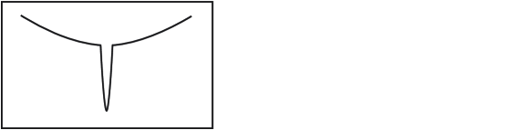
Figure 2: Form of the effective potential.

Hence we expand in terms of the orthonormal eigenfunctions $g(\omega,i,{\bf x})$ of the operator

$${\cal H}_{C} = -{\hbar^{2}\nabla^{2}\over 2m}+(v-u)|\xi({\bf x})|^{2}+(v-2u)\bar{n}({\bf x}).$$ (58)

Here $\hbar\omega$ is the eigenvalue of ${\cal H}_{C}$, and $i$ represents all the other eigenvalues necessary to specify the state. Thus, we write

$$s({\bf x},t) = \sum_{\omega,i}\tilde{s}_{\omega,i}(t)g(\omega,i,{\bf x})$$ (59)

$$gE({\bf x})\xi({\bf x}) = \sum_{\omega,i}I_{\omega,i}g(\omega,i,{\bf x}).$$ (60)

The solution for $\tilde{s}_{\omega,i}(t)$ is then clearly

$$\tilde{s}_{\omega,i}(t) = I_{\omega,i}e^{-i\Omega t}\left(e^{-i(\omega_{2}-\omega_{1}+\omega-\Omega)t}-1\over\hbar(\omega_{2}-\omega_{1}+\omega-\Omega)\right).$$ (61)

The signal from the experiment is proportional to the total occupation, i.e.,

$$\int d^{3}{\bf x}|s({\bf x},t)|^{2} = \sum_{\omega,i}|I_{\omega,i}|^{2}{\sin^{2}[(\omega_{2}-\omega_{1}+\omega-\Omega)t/2]\over[\hbar(\omega_{2}-\omega_{1}+\omega-\Omega)/2]^{2}}$$ (62)

$$\to {2\pi t\over\hbar^{2}}\sum_{\omega,i}|I_{\omega,i}|^{2}\delta(\omega_{2}-\omega_{1}+\omega-\Omega).$$ (63)

The quantity $I_{\omega,i}$ is given by

$$I_{\omega,i} = g\int d^{3}{\bf x}\,g^{*}(\omega,i,{\bf x})\xi({\bf x})E({\bf x}).$$ (64)

At this stage it becomes important to distinguish between the Doppler free case, where $E({\bf x})={\cal E}$, a constant, and the Doppler sensitive case where $E({\bf x})$ has a very rapid oscillation at the wavelength of the light being used, which makes a simple approximation scheme difficult. We do not treat the Doppler-sensitive case in this paper.

5.2 Doppler free excitation

In this case we write

$$I_{\omega,i} = g{\cal E}\int d^{3}{\bf x}\,g^{*}(\omega,i,{\bf x})\xi({\bf x}).$$ (65)

and follow the reasoning of Killian [8], that for relatively high energy excitations such as occur here, the integral of the product of a relatively smooth function, such as $\xi({\bf x})$ and the eigenfunction $g^{*}(\omega,i,{\bf x})$ is dominated by the contribution at the boundary of the classically allowed region, that is from ${\bf x}$ such that

$$\hbar\omega=(v-u)|\xi({\bf x})|^{2}+(v-2u)\bar{n}({\bf x}).$$ (66)

Qualitatively, this occurs because the eigenfunction $g(\omega,i,{\bf x})$ has a behaviour like that of an Airy function near the place where the energy eigenvalue is equal to the potential term in ${\cal H}_{C}$, that is, where $\omega$ satisfies (66). The Airy function and its integral are plotted in Fig.3. Combining (63) and (66), we find that the main contribution comes from positions where

$$\Omega_{C}({\bf x}) = \omega_{2}-\omega_{1}+{(v-u)|\xi({\bf x})|^{2}+(v-2u)\bar{n}({\bf x})\over\hbar}.$$ (67)

5.2.1 Case of a pure condensate

In this case we set $\bar{n}({\bf x})=0$, and our results are the same as those of Killian [8, 9] for a pure condensate.

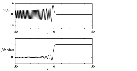
Figure 3: Plot of the Airy function and its integral

5.2.2 Quasiparticle contribution

The remaining equations can be further simplified by noting that because $|v|\gg|u|$, the spatial variation of $p_{n}({\bf x})$ will be very much faster than that of $u_{n}({\bf x})$. Using this, we can make the ansatz

$$p_{n}({\bf x}) = u_{n}({\bf x})\bar{P}({\bf x})$$ (68)

and because of the slow variation of $u_{n}({\bf x})$ we can approximate

$$\nabla^{2}p_{n}({\bf x}) \approx u_{n}({\bf x})\nabla^{2}\bar{P}({\bf x}).$$ (69)

We use this ansatz, and the fact that when $1$ is neglected in comparison to $\bar{N}_{m}$

$$\bar{n}({\bf x}) \approx 2\sum_{m}\bar{N}_{m}u_{m}({\bf x})u_{m}({\bf x}),$$ (70)

to conclude that, for any $n$, the equations (56) become

$$i\hbar{\partial p_{n}({\bf x})\over\partial t}\approx\Big{\{}\hbar(\omega_{2}-\omega_{1})-\mu+H({\bf x})+v[|\xi({\bf x})|^{2}+3\bar{n}({\bf x})]\Big{\}}p_{n}+g{\cal E}u_{n}({\bf x})e^{-i\Omega t}.$$ (71)

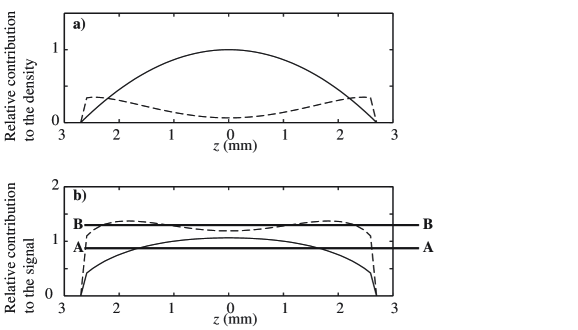
Figure 4: a) Relative condensate (solid line) and quasiparticle (dashed line) contributions to the density; b) Detunings generated by condensate ($\Omega_{C}$, solid line) and quasiparticles ($\Omega_{QP}$, dashed line); see text Sect.6.

The fact that we get the same equation for all $n$ means that there are solutions of this equation of the form (68)—that is, our requirement that $P({\bf x})$ be independent of $n$ is verified. As in the case for equation for the condensate contribution, we can eliminate the chemical potential using (5.1.1), define the operator for the quasiparticles

$${\cal H}_{Q} \equiv -{\hbar^{2}\nabla^{2}\over 2m}+(v-u)|\xi({\bf x})|^{2}+(3v-2u)\bar{n}({\bf x}),$$ (72)

and expand in terms of its eigenfunctions $f(\omega,i,{\bf x})$, using

$$p_{n}({\bf x},t) = \sum_{\omega,i}\tilde{p}_{n,\omega,i}(t)f(\omega,i,{\bf x})$$ (73)

$$g{\cal E}u_{n}({\bf x}) = \sum_{\omega,i}J_{n,\omega,i}f(\omega,i,{\bf x}).$$ (74)

We proceed as for the condensate, and find that the quasiparticle signal is

$$\sum_{n}\int d^{3}{\bf x}\,2\bar{N}_{n}|p_{n}({\bf x})|^{2} = \sum_{n,\omega,i}2\bar{N}_{n}|J_{n,\omega,i}|^{2}{\sin^{2}[(\omega_{2}-\omega_{1}-\omega-\Omega)t/2]\over[\hbar(\omega_{2}-\omega_{1}+\omega-\Omega)/2]^{2}}$$ (75)

$$\to {2\pi t\over\hbar^{2}}\sum_{\omega,i}2\bar{N}_{n}|J_{n,\omega,i}|^{2}\delta(\omega_{2}-\omega_{1}+\omega-\Omega),$$ (76)

where

$$J_{n,\omega,i} = g{\cal E}\int d^{3}{\bf x}f^{*}(\omega,i,{\bf x})u_{n}({\bf x}).$$ (77)

In this case, the functions $u_{n}({\bf x})$ are also very smooth compared to the eigenfunctions, and the integrals will be dominated by contributions from ${\bf x}$ such that

$$\Omega_{QP}({\bf x}) = \omega_{2}-\omega_{1}+{(v-u)|\xi({\bf x})|^{2}+(3v-2u)\bar{n}({\bf x})\over\hbar}.$$ (78)

6 Experimental Comparison

The equations (66,78) can be viewed as the fundamental equations for determining the position in the system from which the measured signal (i.e., the total occupation of the 2S state) originates, although they are definitely only approximations to the equations (50–52). It is apparent the the resonance condition for the condensate component, (66) is significantly different from that of the quasiparticle component, (78), especially as $v\approx-22u$.

In order to evaluate the full signal from the two components, it will be necessary to evaluate the sums (63,76) in the case that the eigenfunctions are almost Airy functions, and this is not a trivial task. In the case that we can approximate the effective potentials by a harmonic approximation, we can show, as in [9, 8], that we can take the intuitive form

$$S(\Omega) \propto \int d^{3}{\bf x}\Big{[}|\xi({\bf x})|^{2}\delta\Big{(}\Omega-\Omega_{C}({\bf x})\Big{)}+\bar{n}({\bf x})\delta\Big{(}\Omega-\Omega_{QP}({\bf x})\Big{)}\Big{]},$$ (79)

in which $\Omega_{C}$ and $\Omega_{QP}$ are given by (67) and (78)

The measured signal is seen form (79) indeed to be the result of an inhomogeneous summation—at a given $\Omega$ the condensate signal (first term) and the quasiparticle signal (second term) come from different regions of the cloud. Using the eigenfunctions from [5] we show in Fig. 4 how this happens. Along the line A–A, corresponding to $\Omega=\Omega_{\rm A}$ the two signals come from very different positions, while at $\Omega=\Omega_{\rm B}$ there is no condensate signal, and the quasiparticle signal is in fact itself derived from multiple positions. What can be seen is that the signal with highest detuning is in fact derived from the quasiparticle component of the signal.

The result of this dual source of the excitation signal is to produce a spectrum which has two very distinctive components, as shown in Fig.6, where the condensate component is qualitatively the same as one would expect from a Thomas-Fermi treatment, and the quasiparticle component is dominated by a large detuning component, which forms a distinct “foot”, protruding from the from the large detuning end of the spectrum. At a given temperature, this feature is more distinct at lower condensate numbers.

The agreement with the experimental data of [4] is rather good. We have taken the total output signal in the form (79), and used the calculated value, (7), of the 1S–2S scattering length, since the results of Sect.3.3 indicate that the apparent value resulting from a measurement in a noncondensed system using the simple $g_{2}=2$ method appropriate to a homogeneous system is likely to be significantly lower than the correct value.

7 Conclusion

We believe that in this paper we have resolved the apparent anomaly, that the hydrogen condensate appeared to be incoherent, and therefore have $g_{2}=2$, rather than $g_{2}=1$, as expected for a true condensate. There are two reasons for the appearance of this anomaly:

• The use of a formalism only strictly valid for the case of a homogeneous untrapped condensate is not justified with the trap geometry employed for the experiment. The time during which the system is illuminated by the exciting illumination must always be significantly shorter than the shortest trap period for this to be valid.

• The more careful treatment of quasiparticle effects leads to higher frequency shifts than would be expected from a treatment based on the assumption that the condensate is pure.

We have also established that the presence of quasiparticles causes a splitting in the resonance, rather than a simple shift, and this leads to a a very characteristic “foot” in the excitation spectrum, of which there is already some experimental evidence.

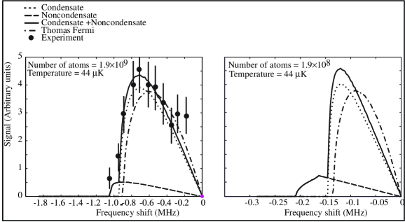
Figure 6: Predicted and measured excitation spectra for a) Parameter regime of the experiments [4, 10]; b) One tenth of the number of condensate atoms. Notice that the “foot” is much more prominent in the latter.

Finally, it must be emphasized that our treatment still makes many approximations. In future work we will include mean-field effects in out computations of eigenfunctions, and shall also develop methods of solving the full equations so derived, including the Doppler sensitive case, which has not been amenable to a simple approximate treatment.

References

References

- [1] Cesar, C. L., Fried, D. G., Killian, T. C., Polcyn, A. D., Sandberg, J. C., Yu, I. A., Greytak, T. J., Kleppner, D., and Doyle, J. M. Phys. Rev. Lett. 77, 2 (1996), 255.
- [2] Cote, R., and Kharchenko, V. Phys. Rev. Lett. 83, 1 (1999), 2100.
- [3] Fried, D. G. Bose-Einstein Condensation of Atomic Hydrogen. PhD thesis, Massachusetts Institute of Technology, 1999.
- [4] Fried, D. G., Killian, T. C., Willmann, L., Landhuis, D., Moss, S. C., Kleppner, D., and Greytak, T. J. Phys. Rev. Lett. 81, 18 (1998), 3811.
- [5] Gardiner, C. W., and Bradley, A. S. Analysis of for the cold-collision frequency shift in the hydrogen condensate experiments. cond-mat/0009371 (revised version), 2000.
- [6] Jamieson, M. J., Dalgarno, A., and Doyle, J. M. Mol. Phys. 87, 1 (1996), 817.
- [7] Jamieson, M. J., Dalgarno, A., and Kimura, M. Phys. Rev. A 51, 1 (1995), 2626.
- [8] Killian, T. C. 1s–2s Spectroscopy of Trapped Hydrogen: The Cold Collision Frequency Shift and Studies of BEC. PhD thesis, Massachusetts Institute of Technology, 1999.
- [9] Killian, T. C. Phys. Rev. A 61 (2000), 033611.
- [10] Killian, T. C., Fried, D. G., Willman, L., Moss, D. L. S. C., Greytak, T. J., and Kleppner, D. Phys. Rev. Lett. 81, 18 (1998), 3807.
- [11] Morgan, S. A. A Gapless Theory of Bose-Einstein Condensation in Dilute Gases at Finite Temperature. PhD thesis, University of Oxford, 1999.
- [12] Morgan, S. A. J. Phys. B 33 (2000), 3847.