On the topological classification of binary trees using the Horton-Strahler index

Abstract

The Horton-Strahler (HS) index $r=\max{(i,j)}+\delta_{i,j}$ has been shown to be relevant to a number of physical (such at diffusion limited aggregation) geological (river networks), biological (pulmonary arteries, blood vessels, various species of trees) and computational (use of registers) applications. Here we revisit the enumeration problem of the HS index on the rooted, unlabeled, plane binary set of trees, and enumerate the same index on the ambilateral set of rooted, plane binary set of trees of $n$ leaves. The ambilateral set is a set of trees whose elements cannot be obtained from each other via an arbitrary number of reflections with respect to vertical axes passing through any of the nodes on the tree. For the unlabeled set we give an alternate derivation to the existing exact solution. Extending this technique for the ambilateral set, which is described by an infinite series of non-linear functional equations, we are able to give a double-exponentially converging approximant to the generating functions in a neighborhood of their convergence circle, and derive an explicit asymptotic form for the number of such trees.

I Introduction

Trees are ubiqutous structures which appear naturally in a large number of physical, chemical, biological and social phenomena, such as river networks, diffusion limited aggregation, pulmonary arteries, blood vessels and tree species, social organizations, decision structures, etc. They also play an important role in computer science (use of registers and computer languages), in graph theory, and in various methods of statistical physics such as cluster expansions and renormalization group.

In spite of their apparent structural simplicity, and the large body of scientific work on trees (a sample of which is found in [2]-[18], [20],[23]-[27] and references therein ), they still offer challenges even related to the quantitative description of their topological structure. At the dawn of the science of complex networks [1], it is therefore rather important to have a complete understanding of all the tree structures and their properties.

A tree is defined as a set of points (vertices, nodes) connected with line segments (branches, or edges) such that there are no cycles or loops (a connected graph without cycles). For the simplest (unlabeled) rooted plane binary tree, each vertex has exactly three connecting branches, except for one vertex which is distinguished from all the others by having only two connecting branches coined as the root (R) of the tree, and a certain number of vertices with a single connecting branch called the ‘leaves’. The height of the tree is defined by the maximum number of levels starting from the root (which has height 0), and it can be calculated as the maximum number of branches one has to pass to reach the root from its vertices (since the leaves have only one branch, it means that this longest excursion must start from one of the leaves). The paths from the leaves to the root define a natural direction on the tree (similarly to the river flow) which is always towards the levels of lower height. A tree of height $k$ we call complete, if it has $2^{k}$ leaves each being a distance $k$ from the root.

Let us now mention three applications of the mathematics of trees which are directly connected to the so-called Horton-Strahler index of the tree, which is the subject of interest of the present paper.

Originally, the Horton-Strahler index of a binary tree was introduced in the studies of natural river networks by Horton [9] and later refined by Strahler [10], as a way of indexing real river topologies, since river networks are topologically similar to binary trees. By definition, a leaf has a rank of 0 (some authors associate the value of 1), and a vertex has a rank of $r=r(i,j)$ where $r(i,j)$ is the index function with $i$ and $j$ being the ranks of the two connecting vertices from the level above. When

$$r(i,j)=\max{(i,j)}+\delta_{i,j},$$ (1)

the index is called the Horton-Strahler index (HS). The quantity of particular interest is the HS index of the root which thus categorizes the topological complexity of the whole tree. Several other quantities can be introduced in relation to the HS index. A segment of order $k$ [11], or a stream of order $k$ [12] is a maximal path of branches connecting vertices of HS index $k$, ending in a vertex with index $k+1$. Let ${\cal S}_{k}(n,T)$ denote the number of segments of order $k$ of a tree $T$ with $n$ leaves, and $<L_{k}(n,T)>$ is the average physical length of a segment of order $k$ (the average $<.>$ is taken on the tree $T$). The bifurcation ratios ${\cal B}_{k}(n,T)$ are defined as ${\cal B}_{k}(n,T)={\cal S}_{k}(n,T)/{\cal S}_{k+1}(n,T)$, and the length ratios via ${\cal L}_{k}(n,T)=<L_{k+1}(n,T)>/<L_{k}(n,T)>$. Horton and Strahler have empirically observed that for river networks both the ${\cal S}_{k}(n)$ and $<L_{k}(n)>$ tend to approximate a geometric series, ${\cal B}_{k}(n)\approx{\cal B}$ with $3\leq{\cal B}\leq 5$ and ${\cal L}_{k}(n)\approx{\cal L}$ with $1.5\leq{\cal L}\leq 3$. Such networks are called topologically self-similar [13]. The notion of HS index is further refined by introducing the biorder $(i,j)$ of a vertex, representing the HS indices of its two children [14],[11], [13], and then studying the ramification matrix, with elements related to the number of vertices with a given biorder.

Another interesting application of the mathematics of binary trees and the HS index, is in the description of the branched structure of diffusion-limited aggregates see Ref. [13] and references therein. In this case the structures are grown on a substrate (which can be a point or a plane) by letting small particles diffuse towards the aggregate where they stick indefinitely at their point of first contact with the cluster. This creates complex and involved branched structures, whose topological complexity still remains a challenging problem to describe.

Finally, the last application we would like to mention is known as the word bracketing problem [5] which has obvious implications in computer science. Let us consider an alphabet of $n$ letters, ${\cal A}=\{Y_{1},Y_{2},...,Y_{n}\}$ and a word $S\equiv x_{1}x_{2}x_{3}..x_{n-1}x_{n}$, $x_{i}\in{\cal A}$. A 2-bracketing of the word $S$ is a partition of its letters (by keeping their order) in groups of two units enclosed in brackets, where a unit can be a letter or a subpartition enclosed in brackets, such as $(x_{1}x_{2})(x_{3}(x_{4}x_{5}))$, or $(x_{1}(x_{2}(x_{3}(x_{4}x_{5})))$, etc. The bracket $(u_{1}u_{2})$ between two units may be associated with a multiplicative composition law $(u_{1}u_{2})=u_{1}\cdot u_{2}\in{\cal A}$. For example let the alphabet ${\cal A}$ be all the positive integers, and the composition law be the regular multiplication of numbers. Then a bracketing of the multiple product $S$ corresponds to one particular way of calculating $S$. A one-to-one correspondence can be made immediately to trees: let the letters ${x_{1},x_{2},...,x_{n}}$ of the word $S$ be associated with the leaves of a binary tree. To a particular bracketing of $S$ it corresponds a particular tree constructed by associating a lower level vertex to a bracketing $(u_{1}u_{2})$ (one may think of the brackets as representing the branches of the tree). The main question is how many ways are there to calculate such a product. If one assumes that the multiplication law is neither associative nor commutative, then the problem is refered to as the Catalan problem, see Ref. [5] for a number of solutions. The number of such bracketings is given by the Catalan numbers, $a_{n}=\frac{1}{n}{2n-2\choose n-1}$. The corresponding set of trees (see Fig.1 for $n=4$) is in fact the set of rooted, unlabeled binary plane trees according to this bijection.

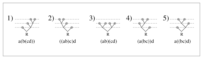
FIG. 1.: The set of rooted, unlabeled binary plane trees corresponding to all the possible non-commutative, non-associative bracketings of the four letter word $abcd$, $n=4$.

For later reference, we mention that the generating function $A(\xi)=\sum_{n=0}^{\infty}\xi^{n}a_{n}$ of the Catalan numbers obey the equation $A^{2}-A+\xi=0$, with $A(0)=0$, so

$$A(\xi)=\frac{1}{2}(1-\sqrt{1-4\xi})\;.$$ (2)

The power series $A(\xi)$ converges within a disk of radius $a_{c}=1/4$.

The problem of enumerating trees becomes more difficult if the composition law is commutative, which was first studied by Wedderburn and Etherington (WE) [6], [7], [8]. In the tree language, this means that two trees are considered identical if after a number of successive reflections with respect to the vertical axes passing through the vertices they can be transformed into each other and in this case they are said to be homeomorphic [4]. For the example shown in Fig. 1, there are only two such trees, since trees 1), 2), 4) and 5) can be transformed into each other. The trees that cannot be transformed into each other are called non-homeomorphic. The set of non-homeomorphic trees is called the set of ambilateral trees, [15], [12]. Let the number of such trees with $n$ leaves be denoted by $w_{n}$. The generating function (GF) defined as $W(\xi)=\sum_{n=0}^{\infty}\xi^{n}w_{n}$ obeys the nonlinear functional equation:

$$W(\xi)=\xi+\frac{1}{2}W(\xi)^{2}+\frac{1}{2}W(\xi^{2})$$ (3)

which has extensively been studied by Wedderburn [6]. Otter [4] studying a more general counting problem where the vertices can have at most $m$ branches comes to the conclusion that for the ambilateral trees, if $n$ is large we have:

$$w_{n}\sim c\;n^{-3/2}\gamma^{n}$$ (4)

where $\gamma=2.4832535...$. The method developed by Otter gives an iterative approach to $c$ and $\gamma$. For example $\gamma$ is

$$\gamma=\lim_{n\to\infty}s_{n}^{2^{-n}}$$ (5)

where $s_{0}=2$, $s_{n}=2+s_{n-1}^{2}$ so that for $n=4$ one already obtains an extremely close value of $\gamma\simeq(2090918)^{2^{-4}}$. Later, Bender developed a more general approach [16] deriving the same results. The coefficient $c$ in (4) can also be computed: $c=0.31877662...$.

The more practical application of the bracketing problem within computer science is the computation of arithmetic expressions by a computer. A general arithmetic expression involving only binary operators can simply be mapped onto a binary tree, called the syntax tree, which has as leaves the operands and the inner vertices the operators. A computer traverses this tree from the leaves towards the root and it uses registers to store the intermediate results. In general there are many ways of traversing such a tree, and the program that uses the minimal number of registers is the most efficient, or optimal one. Ershov has shown [17] that the optimal code will use exactly as many registers to store the intermediate results as the HS index of the associated syntax tree.

In the present paper we investigate how the HS index is distributed on both the rooted, unlabeled, plane binary set of trees, and on the ambilateral set of binary trees. We first answer this question on the rooted, unlabeled, plane binary set, since it is simpler, but it will also provide us with a technique that can be extended to tackle the problem for the ambilateral set. For this set, the question was first answered by Flajolet, Raoult and Vuillemin, [18] with a method somewhat similar to the one presented here. The enumeration problem of the HS index on the ambilateral set is, however, inherently more difficult since it involves functional equations with nonlinear dependence in the argument similar to Eq. (3), and therefore an explicit solution in a closed form becomes impossible to attain. The derivation of an approximant formula for the number of ambilateral trees sharing the same HS index at the root is the main result of this paper.

The paper is organized as follows: first we present our derivation of the enumeration problem for the HS index on the unlabeled set in Section II, and then use this method of derivation from this case to develop a technique that can be used to attack the enumeration problem on the ambilateral set in the asymptotic limit, presented in Section III. Section IV is devoted to conclusions and outlook.

II Distribution of the HS index on the unlabeled set

Let us observe that the root $R$ of the tree has always two subtrees attached to it via the two branches, with $k$ and $n-k$ leaves, respectively, $k=1,2,..,n$. Let $N^{(r)}_{n}$ denote the number of unlabeled trees with $n$ leaves that share the same HS index $r$ at the root. A recursion is found for this number in the light of the observation above:

$$N^{(r)}_{n}=\sum_{k=1}^{n-1}\left\{N^{(r-1)}_{k}N^{(r-1)}_{n-k}+N^{(r)}_{k}\sum_{j=0}^{r-1}N^{(j)}_{n-k}+\right.\left.N^{(r)}_{n-k}\sum_{j=0}^{r-1}N^{(j)}_{k}\right\}$$ (6)

with the conventions $N^{(r)}_{0}\equiv 0$, $N^{(0)}_{n}\equiv\delta_{n,1}$, $N^{(r)}_{1}=\delta_{r,0}$. If the generating function for the variable $n$ is defined as $D_{r}(\xi)=\sum_{n=0}^{\infty}\xi^{n}N^{(r)}_{n}$, then it obeys:

$$D_{r}=D_{r-1}^{2}+2D_{r}\sum_{j=0}^{r-1}D_{j}\;,\;\;r\geq 1,\;\;\;D_{0}=\xi$$ (7)

Next we give an exact solution to (7). Let us introduce the sum $B_{r}\equiv\sum_{j=0}^{r-1}D_{j},\;\;\;r\geq 1,\;\;\;B_{0}=0,\;\;\;B_{1}=\xi\;.$ Then $D_{r}=B_{r+1}-B_{r}$, and after rearranging the terms, Eq. (7) becomes $G_{r}=G_{r-1}$, where $G_{r}=B_{r}^{2}+B_{r+1}(1-2B_{r})$. This means that $G_{r}=G_{0}=\xi$, i.e.,:

$$B_{r}^{2}+B_{r+1}(1-2B_{r})=\xi\;,\;\;\;r\geq 0$$ (8)

Note that the left hand side of (8) remains invariant to $B_{r}\mapsto 1-B_{r}$ which is another solution of (8). However, since in case of the HS index $B_{0}=0$, this latter solution has to be dropped. If we make $2B_{r}\equiv 1-C_{r}$, (8) simplifies to $C_{r}^{2}-2C_{r}C_{r+1}=4\xi-1$. Which, after dividing on both sides by $4\xi-1$, and introducing $Z_{r}\equiv C_{r}/\sqrt{4\xi-1}$, becomes:

$$Z_{r+1}=\frac{Z_{r}^{2}-1}{2Z_{r}}$$ (9)

Let us now write $Z_{r}=\cot(v_{r})$, such that $v_{0}=\arctan{(\sqrt{4\xi-1})}$. Then (9) becomes $\cot(v_{r+1})=\cot(2v_{r})$ which leads to $v_{r+1}=2v_{r}+\pi m$, $m\in\mathbb{Z}$, and which in turn is solved easily. Thus, $Z_{r}=\cot(2^{r}v_{0})$, so one finally obtains:

$$D_{r}(\xi)=\frac{\sqrt{4\xi-1}}{2\sin\left(2^{r+1}\mbox{arctg}\sqrt{4\xi-1}\right)}\;.$$ (10)

Eq. (10) is the exact solution to (7) in the complex $\xi$ plane. On the real axis, within the radius of convergence $a_{c}$ the above expression takes the form: $D_{r}(\xi)=\sqrt{1-4\xi}\big{/}\left[2\mbox{sh}\left(2^{r+1}\mbox{arcth}\sqrt{1-4\xi}\right)\right]$, $\xi<a_{c}=1/4$. Since within the convergence disk one must have $\sum_{r=0}^{\infty}D_{r}(\xi)=A(\xi)$, we just obtained the identity (using (2)):

$$1+\sum_{r=1}^{\infty}\frac{1}{\mbox{sh}(2^{r}x)}=\mbox{cth}{(x)},\;\;\;x>0$$ (11)

This identity can be checked to hold via more direct methods [22]. The singularities of $D_{r}(\xi)$ lie on the positive real axis at:

$$\xi_{k}^{(r)}=\frac{1}{4\cos^{2}(k\pi/2^{r+1})},\;\;k=1,...,2^{r}-1$$ (12)

with an additional singularity at infinity (corresponding to $k=2^{r}$). We certainly have $\xi_{k}^{(r)}>a_{c}$. On the other hand if one simply iterates (7) we obtain:

$$D_{r}(\xi)=\frac{\xi^{2^{r}}}{2^{r}P_{r}(\xi)}$$ (13)

where $P_{r}(\xi)$ is a polynomial in $\xi$ of order $2^{r}-1$: $P_{1}(\xi)=2^{-1}-\xi$, $P_{2}(\xi)=P_{1}(\xi)(2^{-1}-2\xi+\xi^{2})$, $P_{3}(\xi)=P_{2}(\xi)(2^{-1}-4\xi+10\xi^{2}-8\xi^{3}+\xi^{4})$,… etc. One can find an explicit form for this polynomial from the general solution (10) if one invokes the identity [21]: $\sin\left(nx\right)=n\sin x\cos x\prod_{k=1}^{(n-2)/2}\left(1-\sin^{2}x/\sin^{2}(k\pi/n)\right)$, so that (13) is recovered with: $P_{r}(\xi)=\prod_{k=1}^{2^{r}-1}\mbox{ctg}^{2}(k\pi/2^{r+1})(\xi_{k}^{(r)}-\xi)$. It is easy to show, however, that $\prod_{k=1}^{2^{r}-1}\mbox{ctg}^{2}(k\pi/2^{r+1})=1$, so the polynomial simplifies to:

$$P_{r}(\xi)=\prod_{k=1}^{2^{r}-1}(\xi_{k}^{(r)}-\xi)$$ (14)

expression valid on the whole complex $\xi$ plane. Based on the explicit solution we obtained, one can give an exact form to the distribution of the HS index on the unlabeled set of trees, by inverting the generating function via:

$$N^{(r)}_{n}=\frac{1}{2\pi i}\oint\frac{d\xi}{\xi^{n+1}}D_{r}(\xi)=\frac{1}{2\pi i}\oint\frac{d\xi}{\xi^{n+1}}\frac{\xi^{2^{r}}}{2^{r}P_{r}(\xi)}$$ (15)

One can write:

$$\frac{1}{2^{r}P_{r}(\xi)}=\sum_{j=1}^{2^{r}-1}\frac{A_{j}^{(r)}}{\xi_{j}^{(r)}-\xi}$$ (16)

where $A_{j}^{(r)}=2^{-r}\prod\limits_{{k=1\atop k\neq j}}^{2^{r}-1}\left(\xi_{k}^{(r)}-\xi_{j}^{(r)}\right)^{-1},\;\;j=1,...,2^{r}-1$. By Cauchy’s theorem the integrals in (15) are readily performed, and one obtains:

$$N^{(r)}_{n}=\left\{\begin{array}[]{ll}\sum\limits_{j=1}^{2^{r}-1}A_{j}^{(r)}\left[\xi_{j}^{(r)}\right]^{-(n-2^{r}+1)},&n\geq 2^{r}\\ 0,&\!\!\!\!\!0\leq n\leq 2^{r}-1\end{array}\right.\;\;\;\;$$ (19)

From (16) it follows that $\sum_{j=1}^{2^{r}-1}A_{j}^{(r)}/\xi_{j}^{(r)}=2^{-r}/P_{r}(0)=1$. To obtain the last equality we used the form (14) and (12). Thus: $N^{(r)}_{2^{r}}=1,\;\;\;r=1,2,...$ The numbers $A_{j}^{(r)}$ can be calculated as follows: observe that

$$A_{j}^{(r)}=\lim_{\xi\to\xi_{j}^{(r)}}\frac{\xi_{j}-\xi}{2^{r}P_{r}(\xi)}=-\frac{1}{2^{r}P_{r}^{\prime}(\xi_{j}^{(r)})},$$ (20)

where we used the L’Hôpital rule in the last equality. On the other hand from (13) and (10) it follows: $2^{r}P_{r}(\xi)=2\xi^{2^{r}}\sin\left(2^{r+1}\mbox{arctg}\sqrt{4\xi-1}\right)/\sqrt{4\xi-1}$. Taking the derivative of this equation at the point $\xi_{j}^{(r)}$, and inserting it in (20) it yields:

$$A_{j}^{(r)}=(-1)^{j+1}\frac{4\xi_{j}^{(r)}-1}{2^{r+1}[\xi_{j}^{(r)}]^{2^{r}-1}}$$ (21)

Thus, we obtain from (19) the more explicit form

$$N^{(r)}_{n}=\frac{1}{2^{r+1}}\sum\limits_{j=1}^{2^{r}-1}(-1)^{j+1}\frac{4\xi_{j}^{(r)}-1}{[\xi_{j}^{(r)}]^{n}},\;\;\;n\geq 2^{r},$$ (22)

or using (12):

$$N^{(r)}_{n}=\frac{4^{n}}{2^{r+1}}\sum\limits_{j=1}^{2^{r}-1}(-1)^{j+1}\sin^{2}\left(\frac{j\pi}{2^{r+1}}\right)\left[\cos\left(\frac{j\pi}{2^{r+1}}\right)\right]^{2n-2}$$ (23)

an expression first derived by Flajolet et. al. [18]. Following this paper [18], our polynomials $P_{r}$ can be simply connected to the Tchebycheff polynomial $U$ [21], via the relation: $P_{r}(\xi)=2^{-r}\xi^{2^{r}-1/2}U_{2^{r+1}-1}(1/(2\sqrt{\xi}))$.

If one employs the Poisson resummation formula for functions defined on a compact support (see Appendix B in Ref. [19]) on (23), an equivalent combinatorial expression can be derived in the form: $N^{(r)}_{n+1}=\sum_{m=1}^{\infty}\nabla^{2}\big{[}{2n\choose n+k}\big{]}(k)\big{|}_{k=1+(2m-1)2^{r}}$, where $(\nabla f)(k)=f(k)-f(k-1)$ is the finite difference operator. For a different method, see [18].

Scaling limits. Next we briefly present the results of an asymptotic analysis on the $N^{(r)}_{n}$ numbers. Since $N^{(r)}_{n}$ is an enumeration result, it typically contains several scaling limits. In physical processes, during the growth of branched structures, usually only one of these limits is selected, and in frequent cases this limit has self similar properties (such as for DLA, or for random generation of binary trees, [20]). By definition, the family of trees that obey $\lim_{r\to\infty}(\ln{[n(r)]})/r=const.\equiv\ln{{\cal B}}$ is called topologically self similar [13], where ${\cal B}$ is the bifurcation number.
1) $n\to\infty$ and $r$ fixed. In this case the first term in (23) dominates the sum and the asymptotic behavior is given by $N^{(r)}_{n}\sim 2^{-r-1}\mbox{tg}(\pi/2^{r+1})e^{n\ln{[4\cos^{2}(\pi/2^{r+1})]}}$. The rate of the exponential growth is a number between $\ln 2$ and $2\ln 2$. 2) $n\to\infty$, $r\to\infty$, $\sqrt{n}/2^{r}\to\infty$. Here the first term in (23) is still dominant (the rest being exponentially small corrections) and yields: $N^{(r)}_{n}\sim\pi^{2}\;2^{-3(r+1)}\;e^{n\left(2\ln 2-\pi^{2}/4^{r+1}\right)}$. If $\sqrt{n}/2^{r}$ diverges with $r$ slower than exponential, we have topological self similarity with ${\cal B}=4$.
3) $n\to\infty$, $r\to\infty$, $\sqrt{n}/2^{r}\to d$, with some $0<d<\infty$. In this case the rest of the terms in (23) (after the first has been factored out) are of the type $j^{2}e^{-(j-1)\pi^{2}d^{2}}$ and the final expression is: $N^{(r)}_{n}\sim A(d)\;4^{n}n^{-3/2}\;4^{n}$. The topological self similarity is obvious with ${\cal B}=4$. The factor $A(d)$ is given by $A(d)=\pi^{2}e^{-\pi^{2}d^{2}}(1-e^{-\pi^{2}d^{2}})/(1+e^{-\pi^{2}d^{2}})^{3}$.
4)$n\to\infty$, $r\to\infty$, $\sqrt{n}/2^{r}\to 0$, and $n/2^{r}\to\infty$. In this case the analysis is performed easier from the combinatorial expression of $N^{(r)}_{n}$ and yields: $N^{(r)}_{n}\sim\pi^{-1/2}\;n^{-5/2}\;e^{n2\ln 2-4^{r}/n}$.

III Distribution of the HS index on the ambilateral set

Let us now analyze the same question on the set of ambilateral trees, and denote the number of ambilateral trees with $n$ leaves and HS index $r$ by $M^{(r)}_{n}$. We certainly must have the relation

$$\sum_{r=0}^{\infty}M^{(r)}_{n}=w_{n}\;.$$ (24)

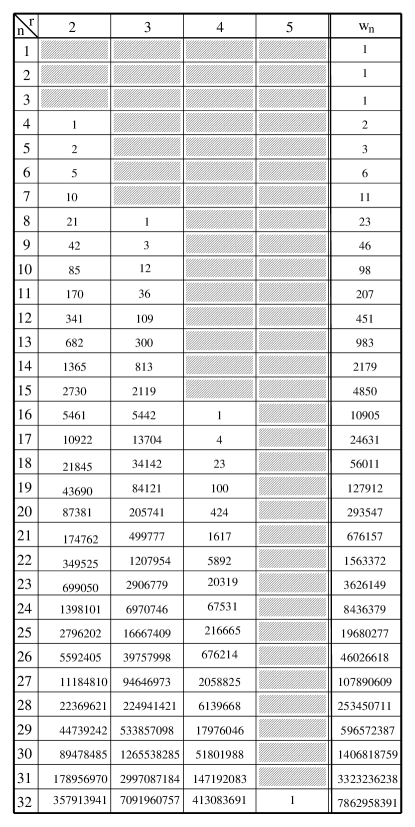
FIG. 2.: Particular values for the number of ambilateral trees with $n$ leaves and HS index $r$. The shaded entries mean that there is no such tree.

The table in Fig. 2 gives the distribution of the HS index for $n$ up to 32 and $r=2,3,4,5$. We can check easily that $M^{(0)}_{n}=\delta_{n,1}$, and $M^{(1)}_{n}=1-\delta_{n,1}$, so for simplicity these are not represented in the table.

The numbers $M^{(r)}_{n}$ obey slightly more complicated recurrence relations since now the counting has to be done on a more restricted set. We must distinguish between odd and even $n$ values. However, the two cases can be combined into one, if the convention $M^{(r)}_{\nu}=0$ for $\nu$ non-integer is adopted. The corresponding recurrence relation becomes:

$$M^{(r)}_{n}=\!\!\!\sum_{0\leq k<j\leq n}\!\!\!\delta_{k+j,n}\Bigg{[}M^{(r-1)}_{k}M^{(r-1)}_{j}+\sum_{s=0}^{r-1}\left(M^{(r)}_{k}M^{(s)}_{j}+M^{(s)}_{k}M^{(r)}_{j}\right)\Bigg{]}+M^{(r)}_{n/2}\sum_{s=0}^{r-1}M^{(s)}_{n/2}+\frac{1}{2}M^{(r-1)}_{n/2}\Big{(}1+M^{(r-1)}_{n/2}\Big{)}$$ (25)

The generating function $V_{r}(\xi)=\sum_{n=0}^{\infty}\xi^{n}M^{(r)}_{n}$ will thus obey:

$$V_{r}(\xi)=\frac{1}{2}\;\frac{\big{[}V_{r-1}(\xi)\big{]}^{2}+V_{r-1}(\xi^{2})}{1-\sum\limits_{s=0}^{r-1}V_{s}(\xi)},\;\;r\geq 1,$$ (26)

and $V_{0}(\xi)=\xi$. As a check for the correctness of (26), let us see if we recover the identity $\sum_{r=0}^{\infty}V_{r}(\xi)=W(\xi)$ (which follows from (24)). Eq. (26) is equivalent to $2V_{r}(\xi)-2\sum_{s=0}^{r-1}V_{s}(\xi)V_{r}(\xi)=\big{[}V_{r-1}(\xi)\big{]}^{2}+V_{r-1}(\xi^{2})$. Introduce the temporary variable $G(\xi)=\sum_{r=0}^{\infty}V_{r}(\xi)$ and sum both sides of the equation over $r$, $r=1,2,..,\infty$. One obtains $2(G(\xi)-\xi)-2\sum_{r=1}^{\infty}\sum_{s=0}^{r-1}V_{s}(\xi)V_{r}(\xi)=\sum_{r=0}^{\infty}\big{[}V_{r}(\xi)\big{]}^{2}+G(\xi^{2})$. Using the identity $2\sum_{r=1}^{\infty}\sum_{s=0}^{r-1}V_{s}\;V_{r}=\left(\sum_{r=0}^{\infty}V_{r}\right)^{2}-\sum_{r=0}^{\infty}V_{r}^{2}$, one finds $G(\xi)=\xi+\frac{1}{2}\big{[}G(\xi)\big{]}^{2}+\frac{1}{2}G(\xi^{2})$ which is precisely Eq. (3), showing that $G(\xi)=W(\xi)$, i.e., the relation $\sum_{r=0}^{\infty}V_{r}(\xi)=W(\xi)$ holds, indeed.

In contrast to the previous case, the functional recurrence (26) cannot be treated in an exact analytical fashion due to the functional dependence on $\xi^{2}$. However, one can derive the asymptotic behaviour and make statements that will lead to rather close approximations of the $M^{(r)}_{n}$ numbers. It is instructive to look at a few particular values, first:

$$V_{1}(\xi)=\frac{\xi^{2}}{1-\xi},$$ (27)

$$V_{2}(\xi)=\frac{\xi^{4}}{(1-2\xi)(1-\xi^{2})},$$ (28)

$$V_{3}(\xi)=\xi^{8}\frac{1-2\xi+\xi^{2}+2\xi^{3}-3\xi^{4}}{(1-2\xi)(1-2\xi^{2})(1-\xi^{4})(1-3\xi+4\xi^{3}-\xi^{4})}\;.$$ (29)

Inverting $V_{2}(\xi)$, one obtains: $M^{(2)}_{n}=\big{[}2^{n-1}-3+(-1)^{n-4}\big{]}/6$, $n\geq 4$, which can be checked to hold, see the table in Fig. 2. The result from the inversion of $V_{3}(\xi)$ is already so complicated that it is not worth presenting. As the index $r$ increases, the polynomial expressions become more and more involved. Figure 3 shows the function $V_{8}(\xi)$ in the interval $[-2.0,2.0]$.

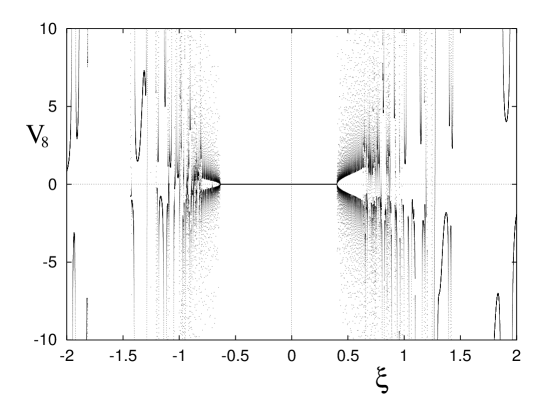
FIG. 3.: The generating function $V_{8}(\xi)$ on the real axis. The function was evaluated in more than $1.3\cdot 10^{5}$ points, and represented by dots.

For every $r$, the power series for $V_{r}(\xi)$ has non-negative coefficients, $M^{(r)}_{n}\geq 0$. Based on a classic theorem of complex analysis, this means that on the circle of convergence, of radius $\alpha_{r}>0$, there will be a singularity of $V_{r}(\xi)$ at $\xi=\alpha_{r}$. Next we show, that we have the ordering $0<\alpha_{r+1}<\alpha_{r}<1$ for $r\geq 2$, and the limit $\lim_{r\to\infty}\alpha_{r}$ exists and it is equal to $\alpha\equiv 1/\gamma=0.4026975036...$. We shall use mathematical induction to prove the ordering. From the particular examples above it follows that $\alpha_{2}=0.5$, $\alpha_{3}=0.424507...$. Let us now assume that $\alpha_{j}<\alpha_{j-1}<1$ for all $j\leq r$, $j\geq 2$. We will show that $\alpha_{r+1}<\alpha_{r}$. Note that the radius of convergence for $V_{j}(\xi^{2})$ is $\sqrt{\alpha_{j}}>\alpha_{j}$, if $\alpha_{j}$ is less than unity. By reductio ad absurdum, let us assume first, that $\alpha_{r+1}>\alpha_{r}$. This means, that $V_{r+1}(\xi)$ is analytic in $\alpha_{r}$. From (26),

$$V_{r+1}(\xi)=\frac{V^{2}_{r}(\xi)+V_{r}(\xi^{2})}{1-V_{0}(\xi)-...-V_{r}(\xi)}\;.$$ (30)

By the argument above, $V_{r}(\xi^{2})$ is analytic in $\alpha_{r}$ (its radius of convergence is $\sqrt{\alpha_{r}}>\alpha_{r}$, since by assumption $\alpha_{r}<\alpha_{r-1}<...<\alpha_{2}=1/2<1$). In the denominator of (30), all functions $V_{j}$, $j=0,1,..r-1$ are analytic in $\alpha_{r}$, because by assumption they all have radii of convergence strictly larger than $\alpha_{r}$. However, $V_{r}$ is singular in $\alpha_{r}$, and the singularities do not cancel in the numerator and denominator of (30), and thus $V_{r+1}$ is singular in $\alpha_{r}$, a contradiction. We are left to prove that $\alpha_{r+1}=\alpha_{r}$ cannot hold. Let us denote $B_{r}=\sum_{s=0}^{r}V_{s}$. Again, we assume, that $\alpha_{r+1}=\alpha_{r}$ is true. It is easy to show, that for any finite $r$, $|V_{r}(\alpha_{r})|=\infty$. This means from the recurrence relation that

$$B_{r-1}(\alpha_{r})=1$$ (31)

(in the numerator of (26) we have only functions analytic at $\alpha_{r}$). Since $V_{r+1}(\xi)=\left[V^{2}_{r}(\xi)+V_{r}(\xi^{2})\right]/[1-B_{r}(\xi)]$, from the assumption $\alpha_{r+1}=\alpha_{r}$ it would follow that the equation $B_{r}(x)=1$ cannot have any solutions ($V_{r+1}$ is analytic within the circle of convergence) in the interval $0<x<\alpha_{r}$. (Note that in the interval $0<x<\alpha_{r}$, the numerator $V^{2}_{r}(\xi)+V_{r}(\xi^{2})$ cannot be zero, since the power series $V_{r}$ has only positive coefficients). The equation $B_{r}(x)=1$ is equivalent to $B_{r-1}(x)+V_{r}(x)=1$. However, from (26) $1-B_{r-1}(x)=\left[V^{2}_{r}(x)+V_{r}(x^{2})\right]/V_{r}(x)$, Thus, the equation

$$V^{2}_{r}(x)=V^{2}_{r-1}(x)+V_{r-1}(x^{2})$$ (32)

should have no solution in $0<x<\alpha_{r}$. If $x$ is arbitrarily close to $\alpha_{r}$, then $V^{2}_{r}(x)$ is arbitrarily large. However, since $\alpha_{r-1}>\alpha_{r}$, $V^{2}_{r-1}(x)$, and $V^{2}_{r-1}(x^{2})$ are both bounded from above. Thus, for $x$ sufficiently close to $\alpha_{r}$, we have $V^{2}_{r}(x)>V^{2}_{r-1}(x)+V_{r-1}(x^{2})$. On the other hand, the HS index of a tree $T$ equals to the height of the largest, complete, balanced tree embedded in $T$. This means, that $M^{(r)}_{n}=0$ for $n=0,1,2,..,2^{r}-1$. Also, $M^{(r)}_{2^{r}}=1$. In other words, one must have $V_{r}(x)=x^{2^{r}}\left(1+{\cal O}(x)\right)$.

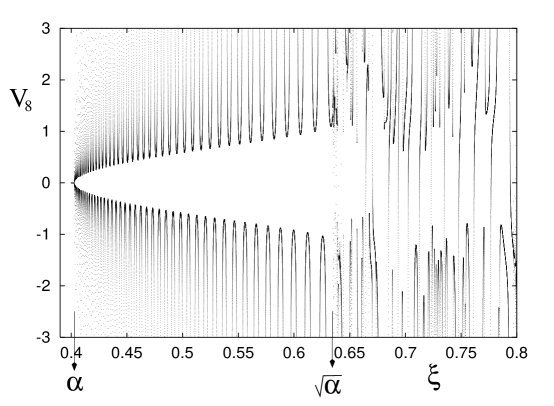
FIG. 4.: A magnified region of Figure 4 The arrows indicate the positions $\alpha=0.40269...$ and $\sqrt{\alpha}=0.63458...$ on the real axis.

This means that $V^{2}_{r-1}(x)=x^{2^{r}}\left(1+{\cal O}(x)\right)$, $V_{r-1}(x^{2})=x^{2^{r}}\left(1+{\cal O}(x^{2})\right)$, and $V^{2}_{r}(x)=x^{2^{r}}x^{2^{r}}\left(1+{\cal O}(x)\right)$. Since $V^{2}_{r-1}(x)+V_{r-1}(x^{2})=2x^{2^{r}}\left(1+{\cal O}(x)\right)$, there will always be an $x>0$, ($x<1$), sufficiently close to zero, such that $V^{2}_{r}(x)<V^{2}_{r-1}(x)+V_{r-1}(x^{2})$. Therefore, there must exist an $0<x<\alpha_{r}$, for which (32) holds, which is a contradiction. Thus, we have proven that $0<\alpha_{r+1}<\alpha_{r}<1$, for all $r\geq 2$. As a matter of fact we have also shown, that the radii of convergence satify:

$$V^{2}_{r}(\alpha_{r+1})=V^{2}_{r-1}(\alpha_{r+1})+V_{r-1}(\alpha_{r+1}^{2}),\;\;\;r\geq 1.$$ (33)

Since the series $\alpha_{r}$ is monotonically decreasing, and bounded from below, the limit $\alpha=\lim_{r\to\infty}\alpha_{r}$ exists.

We have shown that $\sum_{r=0}^{\infty}V_{r}{(\xi)}=W(\xi)$. Since the radius of convergence for the left hand side is the minimum of all the radii of the terms in the summation, i.e., $\alpha$, it must equal to the radius of convergence for $W(\xi)$, which, as shown by Otter and Bender is $1/\gamma$, $\lim_{r\to\infty}\alpha_{r}=\alpha=1/\gamma=0.4026975036...$. Taking the limit $r\to\infty$ in (31), we get

$$W(\alpha)=1$$ (34)

(since by definition $B_{r}=\sum_{s=0}^{\infty}V_{s}$, so $\lim_{r\to\infty}B_{r}=W(\xi)$). Or, using (3):

$$W(\alpha^{2})=1-2\alpha$$ (35)

an identity also shown by Bender. Eqs. (35) and (3) can simply be combined to give the iterative computation of $\alpha$ in the form already mentioned in the Introduction, as follows: if we make the temporary notation

$$U(\xi)\equiv[1-W(\xi)]/\sqrt{\xi}\;,$$ (36)

Eq. (3) takes the form

$$U(\xi^{2})=2+U^{2}(\xi)\;,$$ (37)

and Eq. (35) simplifies to

$$U(\alpha^{2})=2\;.$$ (38)

Let $S(x)=2+x^{2}$. Then, from (37) $U(\xi^{2})=S(U(\xi))$, or $U(\xi)=S(U(\xi^{1/2}))=S(S(U(\xi^{1/4})))=S(...S(U(\xi^{2^{-n}}))...)$, where there are a total of $n$ compositions for the $S$ function, $n$ arbitrary. Let us now choose $\xi=\alpha^{2^{n+1}}$. This means, $U(\alpha^{2^{n+1}})=S(...S(U(\alpha^{2}))...)=S(...(S(2))...)$, by virtue of (38). From (36), $U(\alpha^{2^{n+1}})=[1-W(\alpha^{2^{n+1}})]/\alpha^{2^{n}}$. We have shown previously, that $\alpha<1$ (it is the limit of the monotonically decreasing series $\alpha_{r}<1$), therefore we have:

$$\alpha=\lim_{n\to\infty}\left(\frac{1-W(\alpha^{2^{n+1}})}{s_{n}}\right)^{2^{-n}}=\lim_{n\to\infty}s_{n}^{-2^{-n}}$$ (39)

since $W(\alpha^{2^{n+1}})\to W(0)=0$, and where $s_{n}=S(s_{n-1})$, $s_{0}=2$, just as in the Introduction. The convergence is double-exponential, very fast.

As in Section II, the asymptotic behavior of the $M^{(r)}_{n}$ numbers for relatively large $n$ and $r$ is governed by the innermost singularity of $V_{r}(\xi)$ on the real axis. The graph of $V_{8}$ shown in Figure 3 suggests, that the generating function is in fact well behaved in a certain interval to the right of the radius of convergence, $\alpha_{8}$, see also Figure 4. The existence of this interval comes from the fact that the singularities of the term with nonlinear argument $V_{r-1}(\xi^{2})$ in the numerator of (26) kick in only beyond the circle of convergence of $V_{r-1}(\xi^{2})$, which is $\sqrt{\alpha_{r-1}}>\alpha_{r-1}$. Thus, in the interval $\alpha_{r}<x<\sqrt{\alpha_{r-1}}$ the term with the nonlinear argument is analytic, which ultimately is responsible for this nice behaviour. Because, $\alpha<\alpha_{r-1}$, for convenience we shall define the interval of this nice behaviour to be $I=[\alpha,\sqrt{\alpha})$. In order to exploit this observation, we shall first rewrite the recurrence relation (26). Let us denote $H_{r}(\xi)=1-\sum_{s=0}^{r-1}V_{s}(\xi)$. With this notation, (26) takes the form $G_{r}(\xi)=G_{r-1}(\xi)$, $r\geq 1$, where $G_{r}(\xi)=H^{2}_{r}(\xi)-2H_{r}(\xi)H_{r+1}(\xi)+H_{r}(\xi^{2})$. This leads to the new recurrence:

$$H^{2}_{r}(\xi)-2H_{r}(\xi)H_{r+1}(\xi)+H_{r}(\xi^{2})=2\xi\;,$$ (40)

$H_{0}(\xi)=1$. This would be exactly solvable if it were not for the dependence on the nonlinear argument $\xi^{2}$. Note the resemblance to (8). Let $h_{r}(\xi)=2\xi-H_{r}(\xi^{2})$, which is an analytic function in $I$. We also have $\Delta h_{r}(\xi)=h_{r}(\xi)-h_{r-1}(\xi)=V_{r}(\xi^{2})=\xi^{2^{r}}\left(1+{\cal O}(\xi^{2})\right)$, the latter equality being shown previously. This shows, that in the interval $I$, the $r$-dependence weakens extremely fast, double-exponentially with increasing $r$. As a matter of fact, an upper estimate is

$$\Delta h_{r}(\xi)\leq\alpha^{2^{r-1}}\;.$$ (41)

In particular, $\Delta h_{3}(\xi)\leq 0.0263$, $\Delta h_{4}(\xi)\leq 0.0006916$, $\Delta h_{5}(\xi)\leq 4.79\cdot 10^{-7}$, $\Delta h_{6}(\xi)\leq 2.28\cdot 10^{-13}$, $\Delta h_{7}(\xi)\leq 5.22\cdot 10^{-26}$, etc. Therefore, from the point of view of the asymptotic behavior, the $h_{r}$ functions can be replaced by their asymptotic expression (as $r\to\infty$):

$$h(\xi)=W(\xi^{2})+2\xi-1\;.$$ (42)

Figure 5 shows the functions $h_{r}$ on the interval $I$ for $r=1,2,3,4,5,6$.

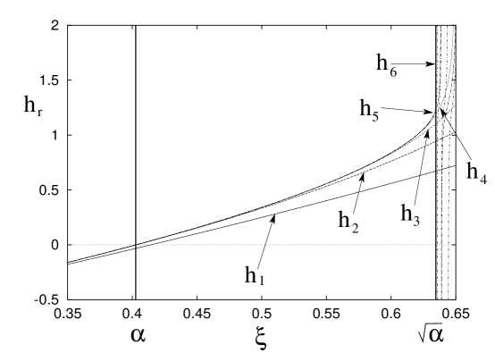
FIG. 5.: The functions $h_{r}(\xi)$ are analytic on $I$. This figure shows $h_{r}(\xi)$ for $r=1,2,3,4,5,6$. The convergence on $I$ to $h(\xi)$ is double-exponentially fast. The thick vertical lines delimit the edges of the interval $I$. Close to $\alpha$, the $h_{r}$ functions cannot be distinguished on $I$ for $r\geq 3$. To the right from $I$ the $h_{r}$ functions develop singularities. The point $\sqrt{\alpha}$ is a left accumulation point for the series of the leftmost singularities of $h_{r}(\xi)$ as $r\to\infty$.

Thus, instead of Eq. (40) we will consider:

$$\overline{H}^{2}_{r}(\xi)-2\overline{H}_{r}(\xi)\overline{H}_{r+1}(\xi)=h(\xi)\;.$$ (43)

The recurrence (43) in turn is easily solved in the way shown in Section I. The result is:

$$\overline{H}_{r}(\xi)=\sqrt{h(\xi)}\;\mbox{ctg}\!\left(2^{r-r_{0}}\mbox{arctg}\left(\frac{\sqrt{h(\xi)}}{\overline{H}_{r_{0}}(\xi)}\right)\right)$$ (44)

where $r_{0}$ for the moment is an arbitrary (positive integer) index. Recurrence (43) will become a good approximation to the recurrence (40) from an index $r_{0}$ on. The larger $r_{0}$ is the more accurate the approximation. Recurrence (43) is applied then with initial condition $\overline{H}_{r_{0}}(\xi)=H_{r_{0}}(\xi)$, which for modest $r_{0}$ values can be obtained by iterating (40) $r_{0}$ times.

What is the error we make when one replaces $h_{r_{0}}(\xi)$ with $h(\xi)$ on $I$? Summing the differences (41) from $r_{0}+1$ to infinity, one obtains the estimate: $h(\xi)-h_{r_{0}}(\xi)\leq\alpha^{2^{r_{0}}}\sum_{m=0}^{\infty}\alpha^{2^{r_{0}}(2^{m}-1)}<\frac{\alpha^{2^{r_{0}}}}{1-\alpha^{2^{r_{0}}}}$. Thus, for example, $h(\xi)-h_{5}(\xi)$ is smaller than $10^{-7}$, $h(\xi)-h_{6}(\xi)$ is smaller than $10^{-13}$, etc.

Therefore, we can finally write on $I$:

$$V_{r}(\xi)\simeq\frac{\sqrt{W(\xi^{2})+2\xi-1}}{\sin{\left(2^{r+1-r_{0}}\mbox{arctg}\left(\sqrt{W(\xi^{2})+2\xi-1}/H_{r_{0}}(\xi)\right)\right)}}\;,\;\;\;r>r_{0}\;,\;\;\;\xi\in I\;.$$ (45)

In Fig. (6) we plot the rhs of (45) and the $V_{r}$ function from iterating (26). Note that the approximation is very good, and it becomes virtually indistinguishable from the true function the closer $\xi$ is to $\alpha$. Larger $r_{0}$ values will also give better approximations, since the approximation is only applied from the $r_{0}$ index on. However, $r_{0}$ cannot be taken too high for approximation purposes, since it assumes that the exact expression of $H_{r_{0}}$ (or $V_{r_{0}}$) is known. This makes only the modest $r_{0}$ values (less than 5) useful. On the other hand, expression (45) is very practical in analysing the singularities of $V$ and give rather close approximant expressions to these singularities. In particular, we see that within the interval $I$, (45) preserves the property that if $\alpha_{r^{\prime}}$ is a singularity of $V_{r^{\prime}}$ (or a zero of $H_{r^{\prime}}$) then it is a singularity of $V_{r}$ (or a zero of $H_{r}$), whenever $r>r^{\prime}$. If one is interested in the asymptotic behavior, then a more tractable expression can be derived for the rhs of (45): the function $h(\xi)$ is analytic on the interval $I$, and since already for modest $r$ values, the innermost singularity of $V_{r}$ (denoted $\alpha_{r}$) is extremely close to $\alpha$, one can safely replace $h(\xi)$ in this neighborhood by: $h(\xi)\simeq h^{\prime}(\alpha)(\xi-\alpha)$.

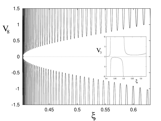
FIG. 6.: The true $V_{r}(\xi)$ function (dashed line) from iterating (26), and the approximation in Eq. (45) (solid line) for $r=8$ with $r_{0}=3$, and $r=3$ with $r_{0}=2$ (the inset).

This leads to the approximant:

$$V_{r}(\xi)\simeq K_{r}(\xi)\equiv\frac{\mu\sqrt{\xi-\alpha}}{\sin{\left(2^{r+1}\mbox{arctg}\left(\theta\sqrt{\xi-\alpha}\right)\right)}}\;,\;\;\;\xi\in I$$ (46)

for sufficiently large $r$ (here “large” means $r\geq 4$) where

$$\mu=\sqrt{h^{\prime}(\alpha)}\;,\;\;\;\;\theta=\frac{\sqrt{h^{\prime}(\alpha)}}{2^{r_{0}}H_{r_{0}}(\alpha)}\;.$$ (47)

Next, we compute $h^{\prime}(\alpha)$. One can use a very similar method to the one employed to obtain (39), to give:

$$h^{\prime}(\alpha)=\lim_{n\to\infty}\frac{s_{n}}{s_{0}s_{1}...s_{n-1}}=3.1710556...$$ (48)

so, $\mu=1.780745815...$. If one computes $\theta$ for $r_{0}=3$, we have $H_{3}(\alpha)=(1-3\alpha+4\alpha^{3}-\alpha^{4})/(1-2\alpha-\alpha^{2}+2\alpha^{3})=0.164518..$, and thus $\theta=1.3530022...$. If we were to use $r_{0}=4$, then one would obtain $H_{4}(\alpha)=0.082262$, so $\theta=1.3529529245$ and slightly improve the approximation on $\theta$. No significant improvement will be obtained with larger $r_{0}$ values. Figure 7 shows the agreement of the form given in (46). For clarity, we defined the function $f(z)$ given by:

$$f(z)=\frac{\mu}{\theta}\frac{\mbox{tg}\left(\frac{z}{2^{r+1}}\right)}{V_{r}\left(\alpha+\theta^{-2}\mbox{tg}^{2}\left(\frac{z}{2^{r+1}}\right)\right)}$$ (49)

Here we use the true $V_{r}$ function using numerical iteration of (26), and evaluate it in the points $\xi=\alpha+\theta^{-2}\mbox{tg}^{2}\left(\frac{z}{2^{r+1}}\right)$. If the approximation (46) is good, then one should have $f(z)=sin(z)$. As seen from Fig. 7 the approximation is already excellent for $r=4$ close to $\alpha$ (which corresponds to the $z=0$ point in this plot). The interval $I$ in these transformed corrdinates corresponds to $(0,2^{r+1}\mbox{arctg}(\theta\sqrt{\sqrt{\alpha}-\alpha}))=(0,0.577435486\cdot 2^{r+1})$. There are no fitting parameters, we used for $\mu$ and $\theta$ the values derived above.

In order to obtain the approximation to the number $M^{(r)}_{n}$ of ambilateral trees with the same HS index at the root, we will have to invert (46). The singularities of the rhs of (46) are given by:

$$\xi^{(r)}_{k}=\alpha+\theta^{-2}\mbox{tg}^{2}\left(\frac{k\pi}{2^{r+1}}\right)\;,\;\;\;k=1,2,3,...,2^{r}-1$$ (50)

(at the moment we do not care whether some of the singularities will fall outside the interval $I$, we just simply want to invert (46), and then at the end keep only those terms from the final expression that were generated by the singularities within $I$).

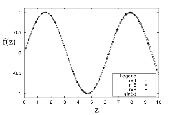
FIG. 7.: The goodness of (46). For $\mu$ and $\theta$ we used the values derived in the text.

In a similar manner to the previous section, we first bring $K_{r}$ to an inverted polynomial form:

$$K_{r}(\xi)=\frac{\mu\left[1+\theta^{2}(\xi-\alpha)\right]^{2^{r}}}{2^{r+1}\theta^{2^{r+1}-1}Q_{r}(\xi)}$$ (51)

where $Q_{r}$ is the polynomial: $Q_{r}(\xi)=\prod_{k=1}^{2^{r}-1}\left(\xi^{(r)}_{k}-\xi\right)$. The case from the previous Section II corresponds to $\mu=1,\theta=2$ and $\alpha=1/4$. Thus, if we denote by $\overline{M}^{(r)}_{n}$ the numbers coming from the inversion of $K_{r}(\xi)$, then:

$$\overline{M}^{(r)}_{n}=\frac{\mu}{\theta^{2^{r+1}-1}}\frac{1}{2\pi i}\oint\frac{d\xi}{\xi^{n+1}}\frac{\left[1+\theta^{2}(\xi-\alpha)\right]^{2^{r}}}{2^{r+1}Q_{r}(\xi)}$$ (52)

We have:

$$\frac{\mu}{2^{r+1}\theta^{2^{r+1}-1}Q_{r}(\xi)}=\sum_{j=1}^{2^{r}-1}\frac{A^{(r)}_{j}}{\xi^{(r)}_{j}-\xi},\;\;\;\mbox{with}\;\;\;A^{(r)}_{j}=\frac{\mu}{2^{r+1}\theta^{2^{r+1}-1}}\prod_{{k=1\atop k\neq j}}^{2^{r}-1}\frac{1}{\xi_{k}^{(r)}-\xi_{j}^{(r)}}.$$ (53)

After performing the integrals, one obtains:

$$\overline{M}^{(r)}_{n}=\sum_{j=1}^{2^{r}-1}A^{(r)}_{j}[\xi_{j}^{(r)}]^{-n-1}\sum_{m=0}^{\min\{n,2^{r}\}}{2^{r}\choose m}(1-\alpha\theta^{2})^{2^{r}-m}\left[\theta^{2}\xi_{j}^{(r)}\right]^{m}$$ (54)

This expression shows that the $\overline{M}^{(r)}_{n}$ may only approximate the ${M}^{(r)}_{n}$ numbers in a certain limit. This is seen from the fact that while one must have ${M}^{(r)}_{n}=0$ for $n<2^{r}$, and ${M}^{(r)}_{2^{r}}=1$, this is not respected by (54) (it would only be respected if $\alpha=\theta^{-2}$, however, this is not the case, and the reason behind this discrepancy is the neglected nonlinearity from the calculations). The limit, in which the approximation becomes good is for $r$ large (it means $r\geq 4$) and $n\gg 2^{r}$. In this case the sum over $m$ can be performed, and one obtains:

$$\overline{M}^{(r)}_{n}=\sum_{j=1}^{2^{r}-1}A^{(r)}_{j}[\xi_{j}^{(r)}]^{-n-1}\left[1+\theta^{2}(\xi_{j}^{(r)}-\alpha)\right]^{2^{r}}$$ (55)

The $A^{(r)}_{j}$ numbers can be calculated in exactly the same way we did in the previous section. This leads to:

$$A^{(r)}_{j}=(-1)^{j+1}\frac{\mu(\xi_{j}^{(r)}-\alpha)}{2^{r}\theta\left[1+\theta^{2}(\xi_{j}^{(r)}-\alpha)\right]^{2^{r}-1}}\;.$$ (56)

Inserting it into (55) it yields:

$$\overline{M}^{(r)}_{n}=\frac{\mu}{2^{r}\theta}\sum_{j=1}^{2^{r}-1}(-1)^{j+1}\frac{\left[1+\theta^{2}\left(\xi_{j}^{(r)}-\alpha\right)\right]\left(\xi_{j}^{(r)}-\alpha\right)}{[\xi_{j}^{(r)}]^{n+1}}$$ (57)

As a check to the correctness of (57) we can take $\mu=1,\theta=2$ and $\alpha=1/4$ from the unlabeled case, to obtain (22). Equation (57) explicitely shows the contribution of each singularity. However, if we want to approximate the $M^{(r)}_{n}$ numbers, we should also account for the condition $\xi^{(r)}_{j}<\sqrt{\alpha}$. Using the expression (50), this leads to $j<J_{r}$, where:

$$J_{r}=\frac{2^{r+1}}{\pi}\mbox{arctg}(\theta\sqrt{\sqrt{\alpha}-\alpha})\simeq(0.1838035250..)\cdot 2^{r+1}$$ (58)

Thus, using again (50):

$$\overline{M}^{(r)}_{n}=\frac{\mu}{2^{r}\theta^{3}}\sum_{j=1}^{[J_{r}]}(-1)^{j+1}\frac{\tan^{2}\!{\left(\frac{j\pi}{2^{r+1}}\right)}\left[1+\tan^{2}\!{\left(\frac{j\pi}{2^{r+1}}\right)}\right]}{\left[\alpha+\theta^{-2}\tan^{2}\!{\left(\frac{j\pi}{2^{r+1}}\right)}\right]^{n+1}}$$ (59)

When the asymptotic limit is generated by the innermost root $\alpha_{r}\simeq\xi^{(r)}_{1}$, i.e., by the first term in (59), one obtains for the topologically self similar ambilateral trees, the scaling behaviour:

$$\overline{M}^{(r)}_{n}\sim\frac{2\mu\pi^{2}d^{3}}{\alpha\theta^{3}}e^{-\frac{\pi^{2}d^{2}}{\alpha\theta^{2}}}n^{-3/2}\gamma^{n}$$ (60)

and therefore ${\cal B}=\gamma=1/\alpha=2.4832535..$.

Let us now see how well formula (59) approximates the ${M}^{(r)}_{n}$ numbers. To do this, we shall define the error $Q^{(r)}_{n}=\left[|\overline{M}^{(r)}_{n}-M^{(r)}_{n}|/M^{(r)}_{n}\right]\cdot 100\%$. For example from the Table in Fig. 2, $M^{4}_{32}=413083691$. The formula above gives $[\overline{M}^{(4)}_{32}]=445781858$, and thus $Q^{(4)}_{32}=7.915...\%$. Further error values: $Q^{(5)}_{100}=5.34132...\%$, $Q^{(5)}_{800}=0.05391...\%$, $Q^{(6)}_{800}=0.003551...\%$.

IV Conclusions and outlook

Combinatorial enumeration of trees is typically difficult to solve when the set under enumeration obeys symmetry-exclusion principles, such as for the ambilateral case treated here. These symmetry-based constraints may arrise in realistic situations and thus forces us to enumerate classes of subsets of trees. In the ambilateral case a class is defined as being formed by those binary trees that have the same number of leaves and HS index at the root and can be obtained one from another via successive reflections with respect to the nodes of the tree. Certainly, the symmetry operation defining the class must be an invariant transformation of the topological index (HS in our case). An other example of such symmetry-operation-generated class-enumeration is the case of the “leftist trees” playing an important role in the representation of priority queues, first shown by Crane [23], followed by Knuth [24], who gives their explicit definition. An elegant enumeration for the leftist trees, using generating function formalism was only given very recently by Nogueira [25].

The existing solutions to such class-enumerations on trees (such as ours and that of Flajolet et. al. [18] and of Nogueira [25]) are obtained via methods taylored for the particularities of the set and symmetry operation in question. It is desirable to have, however, at least on a formal level, a general encompassing theory of class-enumerations of topological indices. In this direction, powerful methods such as that of the antilexicographic order method developed by Erdős and Székely [26], or the method of bijection to Schröder trees developed by Chen [27] may turn to be effective after a suitable extension to include topological indices such as the Horthon-Strahler index. This, however, stands as an open problem.

REFERENCES

[1] A.-L. Barabási, Phys. World, 14, art. 9;
S. H. Strogatz, Nature, 410, 268 (2001).