Superconductivity and Quantum Phase Transitions in Weak Itinerant Ferromagnets

Abstract

It is argued that the phase transition in low-$T_{c}$ clean itinerant ferromagnets is generically of first order, due to correlation effects that lead to a nonanalytic term in the free energy. A tricritical point separates the line of first order transitions from Heisenberg critical behavior at higher temperatures. Sufficiently strong quenched disorder suppresses the first order transition via the appearance of a critical endpoint. A semi-quantitative discussion is given in terms of recent experiments on MnSi and UGe₂. It is then shown that the critical temperature for spin-triplet, p-wave superconductivity mediated by spin fluctuations is generically much higher in a Heisenberg ferromagnetic phase than in a paramagnetic one, due to the coupling of magnons to the longitudinal magnetic susceptibility. This qualitatively explains the phase diagram recently observed in UGe₂ and ZrZn₂.

1 Introduction

In this paper we convey two messages: In the first part we argue that in sufficiently clean samples, and at sufficiently low temperatures, the ferromagnetic phase transition in itinerant electron sytems is generically of first order. In the second part, we provide a physical explanation for the observed structure of the phase diagram in UGe₂ and ZrZn₂, where superconductivity is observed to coexist with ferromagnetism.

1.1 Multicritical points in Itinerant Ferromagnets

The thermal paramagnet-to-ferromagnet transition at the Curie temperature is usually regarded as a prime example of a continuous or second order phase transition: Upon cooling, the magnetization increases continuously from zero above the Curie temperature, to finite values below the Curie point. For materials with high Curie temperatures this behavior is well established.

Recently there has been a considerable interest in the corresponding quantum phase transition of itinerant electrons, that takes place at zero temperature as a function of some non-thermal control parameter. Understanding the quantum phase transition is important, since it controls large parts of the critical behavior that is observable in systems with nonzero, but low, Curie temperatures. There is experimental evidence that in sufficiently clean itinerant ferromagnets the phase transition is discontinuous, or of first order, provided that the Curie temperature is low enough. Specific systems exhibiting this behavior include, MnSi[1] and UGe₂.[2] In both of these systems the transition temperature can be tuned to zero by varying the pressure. It is found that there is a critical pressure, $p_{c}$, above which the ferromagnetic phase transition is discontinuous. An example of a phase diagram is shown in Fig. 1.

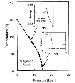
Figure 1: Phase diagram of MnSi. The insets show the behavior of the susceptibility close to the transition. (After Ref. Pfleiderer_et_al).

In the first part of this paper, Sec. 2, we review a general reason for why we expect all sufficiently clean itinerant electron systems to have a discontinuous ferromagnetic transition, if the transition temperature is low enough.

1.2 Coexistence of Ferromagnetism and Superconductivity

At first glance, and according to conventional wisdom, ferromagnetism and superconductivity seem incompatible with one another. For superconductivity with conventional s-wave pairing, the large internal magnetic field inside a magnet would make this singlet pairing energetically very costly. Triplet p-wave pairing, with the spins aligned with the magnetism, is a possibility, but since superconductors tend to expel magnetic flux, one is, again, naively led to the conclusion that superconductivity and ferromagnetism are likely incompatible.

Nevertheless, recent experiments indicate that in some very pure systems, and at very low temperatures, ferromagnetism and superconductivity can coexist, with the same electrons that cause the magnetism also responsible for the superconductivity. So far this phenomenon has been observed in two systems, UGe₂[2] and ZrZn₂,[3] and it is believed to be generic.

These experiments raise a number of obvious questions. First, what is the nature of the superconducting pairing? Does it have s-wave, p-wave, or some other symmetry? What is the nature of the superconducting state? The Meissner effect leads one to believe that the superconducting state must be inhomogeneous. On a more microscopic level, what is the pairing mechanism? In analogy with the phonon mechanism for conventional superconductivity, it was argued theoretically already in the 1960’s that magnetic fluctuations could induce pairing.[4] These theories led to phase diagrams with superconducting phases that appeared more or less symmetric around the ferromagnetic phase boundary.[5] The basic idea behind these theories was that the magnetic fluctuations are largest near a continuous magnetic phase transition, and if a fluctuation induced superconducting state is to be obtained, then it will most likely exist near the magnetic phase boundary. These old theories are in conflict both with our suggestion that the low-temperature ferromagnetic transition is discontinuous in the very pure systems needed to observe superconductivity, and with the experimental observation that the superconducting state is observed only on the ferromagnetic side of the magnetic phase boundary. A schematic phase diagram is shown in Fig. 2.

Figure 2: Schematic phase diagram showing the paramagnetic (PM), ferromagnetic (FM), and superconducting phases (SC) in a temperature (T) - control parameter (CP) plane. (a) shows the qualitative prediction of paramagnon theory, Ref. FayAppel, and (b) qualitatively shows the phase diagram as observed in UGe₂, Ref. Saxena_et_al.

In the second part of this paper, Sec. 3, we review a general pairing mechanism that leads to the conclusion that one should expect a p-wave paired superconducting state to effectively exist only on the ferromagnetic side of the phase boundary, consistent with the experimental observations.

2 Ferromagnetism in clean itinerant systems

On general grounds, Landau[6] argued that as a function of the magnetization $m$, the free energy for small $m$ is of the form

$$F=t\,m^{2}+u\,m^{4}+O(m^{6})\quad.$$ (1)

Within Landau theory, this holds independently of whether one deals with a magnet at zero or finite temperature. In Eq. (1), $t$ is some dimensionless distance from the critical point, and $u$ is assumed to be a positive constant. This equation implies a continuous paramagnetic-to-ferromagnetic phase transition at $t=0$ ($t<0$ describes the ferromagnetic phase and $t>0$ the paramagnetic one) with mean-field critical exponents. It is well known that in general fluctuations effects modify this result for systems whose spatial dimensionality is less than an critical upper dimension, $d_{c}^{+}$, resulting in a continuous phase transition with critical exponents that depend on the spatial dimension as well as the dimension of the order parameter.[7] In effect, Landau’s reasoning breaks down because the free energy is not an analytic function of the magnetization at the critical point. Another well-known, but non-generic mechanism that can invalidate Eq. (1) is that for some systems the coefficient $u$ in Eq. (1) can be negative. In that case one needs to keep the term of $O(m^{6})$ in the free energy, and the transition is discontinuous, or of first order. The point in the phase diagram where $u$ changes sign, as a function of some microscopic parameter, is known as a tricritical point.

This general picture was not expected to be modified if the transition took place at zero rather than finite temperatures. Indeed, the only expected change was that the value $d_{c}^{+}$ would be changed for a zero-temperature transition compared to its thermal counterpart.[8] This expectation turned out to be incorrect, at least for itinerant ferromagnets. The basic reason for its breakdown is that, in a zero temperature itinerant electron system, soft modes that are unrelated to the critical order parameter (OP) or magnetization fluctuations couple to the latter. This leads to an effective long-range interaction between the OP fluctuations, which in turn leads to a nonanalytic magnetization dependence of the free energy, unrelated to the nonanlyticities due to critical fluctuations.[9] In disordered systems, the additional soft modes are the same ‘diffusons’ that cause the so-called weak localization effects in paramagnetic metals.[10] In clean systems, they are ballistic modes that lead to corrections to Fermi liquid theory.[11]

To see these effects we consider the functional form of the free energy of a bulk itinerant ferromagnet at finite temperatures, in the absence of quenched disorder (for a discussion including the effects of disorder, see Ref. us_fm_dirty). In Ref. us_fm_clean it was shown that at $T=0$ there is a contribution to the free energy from the additional soft modes that is schematically given by an integral over a frequency $\omega$ and wavenumber $k$,

$$f(m)=-m^{4}\int_{0}^{\Lambda}dk\,k^{d-1}\int_{0}^{\infty}d\omega\,\frac{1}{[(\omega+k)^{2}+m^{2}]^{2}}\quad.$$ (2)

Here $\Lambda$ is a cutoff, and the crucial sign of this contribution will be discussed below. Equation (2) gives $f(m\rightarrow 0)\propto-m^{d+1}$ for $1<d<3$, and $f(m\rightarrow 0)\propto m^{4}\ln m$ in $d=3$. From now on, we restrict ourselves to the $d=3$ case. The leading effect of a nonzero temperature is adequately represented by replacing $\omega\rightarrow\omega+T$ in the integrand. The net result is that at low temperatures the Landau free energy given by Eq. (1) is generalized to[12]

$$F=t\,m^{2}+v\,m^{4}\ln(m^{2}+T^{2})+u\,m^{4}+O(m^{6})\quad.$$ (3)

The sign of the coefficient $v$ in Eq. (3) warrants some attention. The derivation of the term to leading order in the electron-electron interaction ($O(\Gamma_{t}^{2})$, with $\Gamma_{t}$ a spin-triplet interaction amplitude) yields $v>0$.[12] We further note that $v>0$ indicates a decrease in the tendency towards magnetism due to correlation effects. This can be seen by remembering that $F$ can be related to the magnetic susceptibility. It is well known that correlation effects in general decrease the tendency toward ferromagnetism, so our perturbative results seems to be the generic one. In what follows we therefore assume that $v>0$.

We next analyze the equation of state that follows from Eq. (3). At $T=0$, the transition is clearly of first order, since $m^{4}\ln m<0$ for small $m$.  The transition occurs at $t=v\exp[-(1+u/v)]>0$, and the magnetization at the transition is $m=\exp[-(1+u/v)/2]$. Since we have truncated the OP expansion in Eq. (3), these results are exact only for $u/v>>1$, but similar results are expected when this inequality is not satisfied.

At nonzero $T$, the free energy is an analytic function of $m$, but for small $T$ the coefficients in an $m$-expansion become large. There is a tricritical point at $T_{tc}=\exp(-u/2v)$, with a first order transition for $T<T_{tc}$, and a line of Heisenberg critical points for $T>T_{tc}$. These results, at $T=0$ and $T>0$, lead to a phase diagram as given in Fig. 1. We stress that, since the nonanalytic term in Eq. (3) is due to the long-wavelength excitations in the itinerant electron system, the phase diagram is expected to be generic.

If one adds a finite amount of quenched disorder, the predicted phase diagram becomes quite complicated. Most importantly, a sufficient amount of quenched disorder causes the transition to become continuous. This behavior and the associated critical endpoint (and multicritical points) as well as other features of the phase diagram are discussed in Ref. us_1st_order.

3 Spin-fluctuation induced superconductivity in ferromagnets

In order to study ferromagnetic spin-fluctuation induced superconductivity, we choose an OP field for the superconductivity as ${\cal F}(x,y)=\psi_{\uparrow}(x)\psi_{\uparrow}(y)$, assuming that the magnetization in the ferromagnetically ordered phase is in the z-direction. Here $\psi_{\sigma}(x)$ is an electronic field with spin index $\sigma$ and space-time index $x$. The OP, i.e. the expectation value $\langle{\cal F}(x,y)\rangle\equiv F(x-y)$, is the anomalous Green’s function. At this point the orbital symmetry of the OP is unspecified, but we eventually choose p-wave pairing. Note, that in choosing the above OP we have assumed a particular form of triplet pairing which, as noted in the Introduction, is the most likely superconducting state. For simplicity, and to get a first handle on the theory, we will also assume that the superconducting state is homogeneous. This assumption, as was also noted in the Introduction, is questionable, and its consequences warrant further investigation. Finally, we will not be concerned that ordinary classical critical phenomena might lead to nontrivial magnetic fluctuations close to the magnetic phase boundary because, as pointed out in Sec. 2 above, we expect a discontinuous magnetic phase transition at low temperatures. Further, as we will see below, even if the predicted tricritical point was at inaccessibly low temperatures, so that the transition were effectively always continuous, large scattering very near the transition suppresses the superconducting state very close to the continuous phase boundary anyway.[5, 13, 14]

Using a field theoretic approach, and working to leading order in magnetic fluctuations, we have derived coupled equations of motion for $F$ and the normal Green function, $G_{\sigma}(x-y)=\langle{\bar{\psi}}_{\sigma}(x)\,\psi_{\sigma}(y)\rangle$, that lead to an equation of state for the superconducting OP. In an approximation analogous to Eliashberg theory for conventional superconductivity, we obtain for the linearized gap equation that determines the superconducting critical temperature $T_{c}$,

$$\Delta(p) = \Gamma_{t}T\sum_{k}\chi_{L}(p-k)|G_{\uparrow}(k)|^{2}\Delta(k)\quad,$$ (4)

$$G_{\sigma}(p) = 1/\left[i\omega_{n}-\xi_{\bf p}-\Sigma_{\sigma}(p)\right]\quad,$$ (5)

$$\Sigma_{\sigma}(p) = \Gamma_{t}T\sum_{k}\left[\chi_{L}(p-k)\,G_{\sigma}(k)+2\chi_{T}(p-k)\,G_{-\sigma}(k)\right]\quad.$$ (6)

Here we work in Fourier space, with $p=({\bf p},i\omega_{n})$ comprising the momentum and the Matsubara frequency, and $\sigma=+,-\equiv\uparrow,\downarrow$. $\xi_{\bf p}=\epsilon_{\bf p}-\mu$ is the bare quasiparticle spectrum minus the chemical potential, $\Sigma$ is the normal self-energy, $\Gamma_{t}$ is the spin-triplet interaction amplitude, $\chi_{L,T}$ are the longitudinal and transverse magnetic susceptibilities, respectively, and $\Delta$ is the anomalous self-energy. Note that in the paramagnetic phase, $\chi_{L}=\chi_{T}$ and $G_{\uparrow}=G_{\downarrow}$.

We have solved Eqs. (4) - (6) in a simple McMillan-type approximation. We find for the superconducting transition temperature[15]

$$T_{c}=T_{0}(t)\,\exp\left[-(1+d_{0}^{L}+2d_{0}^{T})/d_{1}^{L}\right]\quad.$$ (7)

Here $T_{0}(t)$ is some measure of the magnetic excitation energy. Following Ref. FayAppel, we use the prefactor of $|t|$ in Eqs. (12) and (13) below,

$$T_{0}(t)=T_{0}\,[\Theta(t)\,t+\Theta(-t)\,5|t|/4]\quad,$$ (8)

with $T_{0}$ a microscopic temperature scale that is related to the Fermi temperature (for free electrons) or a band width (for band electrons). This qualitatively reflects the suppression of the superconducting $T_{c}$ near the FM transition due to effective mass effects[13, 5, 14].

Specializing to the p-wave case, the $d_{0,1}^{L,T}$ read

$$d_{1}^{L} = \left(\Gamma_{t}N_{F}^{\uparrow}/(k_{F}^{\uparrow})^{2}\right)\int_{0}^{2k_{F}^{\uparrow}}dk\,k\,\left(1-\left(k^{2}/2(k_{F}^{\uparrow})^{2}\right)\right)\,D_{L}(k,i0)\ ,$$ (9)

$$d_{0}^{L} = \left(\Gamma_{t}N_{F}^{\uparrow}/(k_{F}^{\uparrow})^{2}\right)\int_{0}^{2k_{F}^{\uparrow}}dk\,k\,D_{L}(k,i0)\quad,$$ (10)

$$d_{0}^{T} = \left(\Gamma_{t}N_{F}^{\uparrow}/(k_{F}^{\uparrow})^{2}\right)\int_{k_{F}^{\uparrow}-k_{F}^{\downarrow}}^{k_{F}^{\uparrow}+k_{F}^{\downarrow}}dk\,k\,D_{T}(k,i0)\quad.$$ (11)

$k_{F}^{\uparrow}(k_{F}^{\downarrow})$ are the Fermi wavenumbers for the up (down)-spin Fermi surface, and $N_{F}^{\uparrow}$ is the density of states at the up-spin Fermi surface. In the paramagnetic phase, $k_{F}^{\uparrow}=k_{F}^{\downarrow}\equiv k_{F}$. $D_{L,T}(q)$ are the longitudinal and transverse (para)magnon propagators, which are related to the electronic spin susceptibility $\chi$ via $D_{L,T}(q)=\chi_{L,T}(q)/2N_{F}$, with $N_{F}$ the density of states at the Fermi level in the paramagnetic phase. In order to perform the integrals we need to specify the susceptibilities. We use the expressions that were derived in Ref. us_fm_mit, with one crucial modification that we will discuss below. In the paramagnetic phase, in the limit of small wavenumbers,

$$D_{L,T}({\bf q},i0)=1/\left[t+b_{L,T}({\bf q}/2k_{F})^{2}\right]\quad,$$ (12)

with $b_{L}=b_{T}$ and $k_{F}$ the Fermi wavenumber. In the Gaussian approximation of Ref. us_fm_mit, $b_{L}=b_{T}=1/3.$ However, more generally we note that Eq. (12) is expected to be a generic form in the long wavelength limit with the $b^{\prime}s$ of $O(1)$. Similarly, in the long wavelength limit, in the ferromagnetic phase,

$$D_{L}({\bf q},i0) = 1/\left[5|t|/4+b_{L}({\bf q}/2k_{F})^{2}\right]\quad,$$ (13)

$$D_{T}(q) = \frac{\Delta/4\epsilon_{F}}{(1-t)^{2}}\left(\frac{1}{i\Omega+(\Delta/2\epsilon_{F})\,b_{T}({\bf q}/2k_{F})^{2}}+{\rm c.c.}\right)\quad,$$ (14)

with $\Delta$ the band splitting energy. The factor $5/4$ in Eq. (13) can be traced back to the fact that the particle number is typically held fixed in experiments. For $0<\Delta<n\Gamma_{t}$, $\Delta$ is related to the magnetization by $m=\mu_{B}\Delta/\Gamma_{t}$, with $n$ the electron density.

Let us discuss the propagators in the magnetic state. The form of the transverse propagator, Eq. (14), is known to be asymptotically exact in the long-wavelength limit, where the spectrum describes the spin-wave or magnon excitations. Equation (13) for the longitudinal propagator, on the other hand, is an RPA or Landau-type approximation that was used in previous theories of magnetic fluctuation induced superconductivity.[5] It is easy to see that this approximation leads to a superconducting phase diagram that is more or less symmetric with respect to the magnetic phase boundary. First, the longitudinal susceptibilities are roughly the same one either side of the transition. Second, the transverse propagators, which are fundamentally different in the two phases, only weakly couple to the superconducting gap equation well inside the magnetic phase where $m$ is not too small. The conclusion is that apart from simple factors, the linearized gap equation is basically the same on both sides of the magnetic phase transition.

We next consider the longitudinal propagator in the ferromagnetic phase in more detail. In a Heisenberg ferromagnet (or in any magnet with a continuous rotation symmetry in spin space), the transverse spin waves or magnons are massless and couple to the longitudinal susceptibility $\chi_{L}$.[17] This effect is most easily illustrated within a nonlinear sigma-model description of the ferromagnet,[18] which treats the order parameter ${\bf m}$ as a vector of fixed length $m$, and parametrizes it as ${\bf m}=m(\pi_{1}(x),\pi_{2}(x),\sigma(x))$, with $\sigma^{2}+\pi_{1}^{2}+\pi_{2}^{2}=1$, and $m$ the magnetization. The diagonal part of the transverse or $\pi$ propagator, $\langle\pi_{i}\pi_{i}\rangle=(m^{2}/2N_{F})D_{T}$, is proportional to the transverse propagator $D_{T}$, and the off-diagonal part has been calculated in Ref. BKMV. The longitudinal propagator, $D_{L}=(m^{2}/2N_{F})\left\langle\sigma(x)\sigma(y)\right\rangle$, can be expanded in a series of $\pi$-correlation functions as,

$$\left\langle\sigma(x)\sigma(y)\right\rangle=1-\left\langle\pi_{i}(x)\pi_{i}(x)\right\rangle+\frac{1}{4}\left\langle\pi_{i}(x)\pi_{i}(x)\pi_{j}(y)\pi_{j}(y)\right\rangle+\ldots$$ (15)

where the repeated indices are summed over. At one-loop order, the term of order $\pi^{4}$ yields the diagram shown in Fig. 3.

Figure 3: Mode-mode coupling contribution to the longitudinal (L) propagator $D_{L}$ from the transverse (T) ones.

Power counting shows that at nonzero temperature, and for dimensions $d<4$, this contribution causes the homogeneous longitudinal susceptibility to diverge everywhere in the ferromagnetic phase, so $\chi_{L}$ is fundamentally different in the ferromagnetic phase than in the paramagnetic one.[17] Ultimately this implies the superconducting transition temperature can be very different in the two phases, and it is this aspect that previous theories missed.

More generally, this one-loop contribution, together with the zero-loop one, Eq. (13), yields a functional form for $D_{L}$ in the ferromagnetic phase that is asymptotically exact at small wavenumbers. This diagram has no analog in the paramagnetic phase, while all other renormalizations of the propagators will give comparable contributions in the ferromagnetic and paramagnetic phases. It is therefore reasonable to calculate $T_{c}$ based one this one-loop result in the ferromagnetic phase, and compare it to the zero-loop calculation in the paramagnetic phase.

In the McMillan approximation noted above, two examples of the resulting phase boundaries for superconductivity in the paramagnetic and ferromagnetic phases are shown in Figs. 4 and 5.

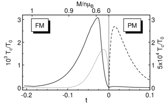
Figure 4: Superconducting $T_{c}$ (solid curve, left scale) as a function of the distance from the critical point $t$, and the magnetization $M$. The dashed line (right scale) shows $T_{c}$ in the paramagnetic phase scaled by a factor of 50, and the dotted curve (right scale) is the result in the ferromagnetic phase without the mode-mode coupling effect. From Ref. us_UGe_2.

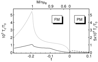
Figure 5: Same as Fig. 2, but for different parameter values (see the text). From Ref. us_UGe_2.

In both figures, the characteristic temperature $T_{0}$ is given by either the Fermi temperature or a band width, depending on the model considered. The magnetization $m$ has been scaled with $\mu_{B}n$, with $\mu_{B}$ the Bohr magneton. The solid line represents the superconductivity $T_{c}$ in the ferromagnetic phase as a function of the distance $t$ from an assumed continuous ferromagnetic critical point. Since the transition is discontinuous, the region very close to the point $t=0$ should be ignored. The dashed line shows the result in the paramagnetic phase scaled by a factor of 50 (right hand scale), and the dotted curve in the ferromagnetic phase (also scaled by a factor of 50, right-hand scale) represents the result that is obtained in the ferromagnetic phase upon neglecting the mode coupling contribution to $\chi_{L}$ given by Fig. 3. In Fig. 4 the values $b_{L}=0.23$ and $b_{T}=0.4$ are used, while in Fig. 5 the values $b_{L}=b_{T}=1$ are used. In both cases, note that the maximum $T_{c}$ in the ferromagnetic phase is $50$ to $100$ times higher than in the paramagnetic phase.

We conclude that for reasonable parameter values, theoretically the effective superconducting phase diagram is given by Fig. 2, consistent with current experimental observations.

4 Discussion

We conclude with a summary of our results, and then briefly discuss several open questions.

We have made two distinct general points. The first result was that clean itinerant electronic systems will in general have a tricritical point for the ferromagnetic phase transition at low temperatures. As a corollary, the zero temperature ferromagnetic transition in clean itinerant systems is generically of first order. This result continues to hold for weakly disordered systems, but no quantitative results are available for the amount of disorder that will destroy the first order phase transition. Once the tricritical point has been destroyed by the disorder, the critical exponents at the second order phase transition at finite temperatures are the known classical Heisenberg exponents,[18] and at zero temperature, they have recently been exactly determined in Ref. us_fm_dirty. The second result was that longitudinal fluctuations are intrinsically larger in the ferromagnetic phase than in the paramagnetic phase. This is a crucial point for magnetic fluctuation induced superconductivity. Simple estimates show that the critical temperature for this type of superconductivity in the ferromagnetic phase can easily be fifty times larger than in the paramagnetic one. All of these results are consistent with current experimental observations.

The most intriguing open questions concern the nature of the magnetic fluctuation induced superconducting state, and an understanding of the phase diagram for all temperatures and magnetic fields. As already noted, one expects an inhomogeneous superconducting state. This point has not yet been discussed theoretically for pairing mechanisms that are both electronic in origin, and sensitive to internal magnetic field effects. Another interesting question is whether there are numerous superconducting phases as a function of temperature (and external magnetic fields). Again, since the pairing mechanism is expected to be electronic in origin, and itself sensitive to superconductivity, it is easy to imagine additional superconducting states appearing inside the superconducting phase, as the temperature is lowered. Similarly, the concept of transverse and longitudinal critical external magnetic fields needs to be worked out for these superconducting states.

References

- [1] C. Pfleiderer, G.J. McMullan, S.R. Julian, and G.G. Lonzarich, Phys. Rev. B 55, 8330 (1997).
- [2] S.S. Saxena et al., Nature 406, 587 (2000); A. Huxley et al., Phys. Rev. B 63, 144519 (2001), and references therein.
- [3] C. Pfleiderer et al., Nature 412, 58 (2001).
- [4] K.A. Brueckner, T. Soda, P.W. Anderson, and P. Morel, Phys. Rev. 118, 1442 (1960); P.W. Anderson and W.F. Brinkman, Phys. Rev. Lett. 30, 1108 (1973).
- [5] D. Fay and J. Appel, Phys. Rev. B 22, 3173 (1980).
- [6] L.D. Landau and E.M. Lifshitz, Statistical Physics, Pergamon (Oxford 1980).
- [7] See, e.g., M.E. Fisher in Advanced Course on Critical Phenomena, edited by F.W. Hahne, Springer (Berlin 1983).
- [8] J. A. Hertz, Phys. Rev. B 14, 1165 (1976), and references therein.
- [9] T. R. Kirkpatrick and D. Belitz, Phys. Rev. B 53, 14364 (1996); D. Belitz, T. R. Kirkpatrick, M.T. Mercaldo, and S.L. Sessions, Phys. Rev. B 63, 174427 (2001); ibid. 63, 174428 (2001).
- [10] For a review, see, P.A. Lee and T.V. Ramakrishnan, Rev. Mod. Phys. 57, 287 (1985).
- [11] T. Vojta, D. Belitz, R. Narayanan, and T.R. Kirkpatrick, Z. Phys. B 103, 451 (1997).
- [12] D. Belitz, T.R. Kirkpatrick, and Thomas Vojta, Rev. Lett. 82, 4707 (1999).
- [13] K. Levin and O. Valls, Phys. Rev. B 17, 191 (1978).
- [14] R. Roussev and A.J. Millis, Phys. Rev. B 63, 14504 (2001).
- [15] T.R. Kirkpatrick, D. Belitz, Thomas Vojta, and R. Narayanan, cond-mat/0105627 (Phys. Rev. Lett., in press).
- [16] T.R. Kirkpatrick and D. Belitz, Phys. Rev. B 62, 952 (2000).
- [17] E. Brézin and D.J. Wallace, Phys. Rev. B 7, 1967 (1973).
- [18] See, e.g., J. Zinn-Justin, Quantum Field Theory and Critical Phenomena, Clarendon (Oxford 1989), ch. 27.
- [19] D. Belitz, T.R. Kirkpatrick, A.M. Millis, and T. Vojta, Phys. Rev. B 58, 14155 (1998).