Master equation approach to configurational kinetics of non-equilibrium alloys and its application to studies of L1₀-type orderings

Abstract

We review a series of works where the fundamental master equation is used to develop a microscopical description of evolution of non-equilibrium atomic distributions in alloys. We describe exact equations for temporal evolution of local concentrations and their correlators as well as approximate methods to treat these equations, such as the kinetic mean-field and the kinetic cluster methods. We also describe an application of these methods to studies of kinetics of L1₀-type orderings in FCC alloys which reveal a number of peculiar microstructural effects, many of them agreeing well with experimental observations.

I Introduction

Problems of evolution of non-equilibrium statistical systems attract attention in many areas of physics. These problems are of particular interest for configurational alloy kinetics—the evolution of the atomic distribution in non-equilibrium alloys. The microstructure and macroscopic properties of such alloys, e.g. strength and plasticity, depend crucially on their thermal and mechanical history—for example, on the kinetic path taken during phase transformations. Theoretical treatments of these problems usually employ either Monte Carlo simulation—see e.g. [2]—or phenomenological kinetic equations for local concentrations and order parameters [3, 4, 5]. However, Monte Carlo studies in this field are time consuming, and until now they provided a limited information on the details of the microstructural evolution. Use of the phenomenological kinetic equations is more feasible, and Khachaturyan and co-workers [3, 4, 5] used this approach as a basis for discussing many microstructural effects. However, the phenomenological approach employs a number of unclear approximations—in particular, the extrapolation of linear Onsager equations for weakly nonequilibrium states to the nonlinear region of states far from equilibrium, and the relation between the phenomenological and microscopic approaches is often unclear.

A consistent description of non-equilibrium alloys can be based on the fundamental master equation for the probabilities of various atomic distributions over lattice sites. The idea to employ this equation for studies of phase transformations was first suggested by Martin [6]. For the last decade this approach has been formulated in terms of both approximate and exact kinetic equations [7, 8, 9, 10, 11, 12, 13] and was applied to many concrete problems [7, 8, 9, 10, 11, 12, 13, 14, 15, 16, 17, 18, 19, 20, 21]. In this paper we describe the main ideas and methods of this approach and illustrate them with an application to studies of microstructural evolution under L1₀ (CuAu I)-type orderings in FCC alloys.

II Exact relations

Following Ref. [10] we consider a substitutional alloy that includes atoms of $m$ species ${\rm p}={\rm p}_{1},{\rm p}_{2},\ldots{\rm p}_{m}$, in particular, vacancies for which p=v. Various distributions of atoms over lattice sites $i$ are described by the different occupation number sets $\{n_{{\rm p}i}\}$ where the operator $n_{{\rm p}i}$ is unity when the site $i$ is occupied by a p-species atom and zero otherwise. For each $i$ the sum of operators $n_{{\rm p}i}$ over all species p is unity, thus only $m-1$ of them are independent. It is convenient to mark the independent operators with special symbols, e.g. with greek letters: $(n_{{\rm p}i})_{\rm indep}=n_{\alpha i}$, while the rest operator denoted as $n_{{\rm r}i}$ is expressed via $n_{\alpha i}$:

$$n_{{\rm r}i}=1-\sum_{\alpha}n_{\alpha i}.$$ (1)

The configurationally dependent part of energy $H^{t}$ can be written as

$$H^{t}=\sum_{{\rm pq},i>j}V_{ij}^{{\rm p}{\rm q}}n_{{\rm p}i}n_{{\rm q}j}+\sum_{{\rm pqr},i>j>k}V_{ijk}^{{\rm p}{\rm q}{\rm r}}n_{{\rm p}i}n_{{\rm q}j}n_{{\rm r}k}+\ldots$$ (2)

After elimination of the operators $n_{{\rm r}i}$ according to (1) Eq. (2) yields the interaction Hamiltonian $H$ in terms of only independent operators $n_{\alpha i}$:

$$H=\sum_{\alpha\beta,i>j}v_{ij}^{\alpha\beta}n_{\alpha i}n_{\beta j}++\sum_{\alpha\beta\gamma,i>j>k}v_{ijk}^{\alpha\beta\gamma}n_{\alpha i}n_{\beta j}n_{\gamma k}+\ldots$$ (3)

where effective interactions $v_{i\ldots j}^{\alpha\ldots\beta}$ are linearly expressed via $V_{i\ldots j}^{\rm p\ldots q}$ in (2).

The fundamental master equation for the probability $P$ to find the occupation number set $\{n_{\alpha i}\}=\xi$ is

$$dP(\xi)/dt=\sum_{\eta}[W(\xi,\eta)P(\eta)-W(\eta,\xi)P(\xi)]$$ (4)

where $W(\xi,\eta)$ is the $\eta\rightarrow\xi$ transition probability per unit time. Adopting for this probabilitiy the conventional “thermally activated atomic exchange model” [6, 7], we can express $W(\xi,\eta)$ in (4) in terms of the probabilitiy $W_{ij}^{\rm pq}$ of an inter-site atomic exchange (“jump”) q$j\leftrightarrow{\rm p}i$ per unit time:

$$W_{ij}^{\rm pq}=n_{{\rm p}i}n_{{\rm q}j}\omega_{ij}^{\rm pq}\exp[-\beta(E_{{\rm p}i,{\rm q}j}^{s}-E_{{\rm p}i,{\rm q}j}^{in})]\equiv n_{{\rm p}i}n_{{\rm q}j}\gamma_{ij}^{\rm pq}\exp(\beta E_{{\rm p}i,{\rm q}j}^{in}).$$ (5)

Here $\omega_{ij}^{\rm pq}$ and $E_{{\rm p}i,{\rm q}j}^{s}$ are the “attempt frequency” and the “saddle point energy” assumed to be independent of alloy configuration; $\beta=1/T$ is the reciprocal temperature; $E_{{\rm p}i,{\rm q}j}^{in}$ is the initial (before the jump) configurational energy of jumping atoms, and $\gamma_{ij}^{\rm pq}=\omega_{ij}^{\rm pq}\exp[-\beta(E_{{\rm p}i,{\rm q}j}^{s})]$ is the configurationally independent factor in the jump probability. If we accept for simplicity the pair interaction model, i.e. retain only the first term in Eq. (2), then the operator $E_{{\rm p}i,{\rm q}j}^{in}$ in (5) may be expressed in terms of formal variational derivatives of the hamiltonian (2) over $n_{{\rm p}i}$ and $n_{{\rm q}j}$, $H_{{\rm p}i}^{t}=\delta H^{t}/\delta n_{{\rm p}i}$ and $H_{{\rm p}i,{\rm q}j}^{t}=\delta^{2}H^{t}/\delta n_{{\rm p}i}\delta n_{{\rm q}j}$:

$$E_{{\rm p}i,{\rm q}j}^{in}=n_{{\rm p}i}H_{{\rm p}i}^{t}+n_{{\rm q}j}H_{{\rm q}j}^{t}-n_{{\rm p}i}n_{{\rm q}j}H_{{\rm p}i,{\rm q}j}^{t},$$ (6)

where the last term corresponds to the substraction of the “double-counted” interaction between the jumping atoms. The employed neglection of a possible configurational dependence of $\gamma_{ij}^{\rm pq}$ in (5) is actually not essential, and one can also use any form of $W_{ij}^{\rm pq}$ obeying the detailed balance principle.

It has been shown in [10] that in studies of practically interesting problems the true vacancy-mediated atomic exchange mechanism can usually be replaced by some equivalent direct exchange model. For example, instead of a real binary alloy ABv with vacancies and the vacancy-mediated atomic exchanges A$\leftrightarrow$v and B$\leftrightarrow$v we can consider a more simple model of a binary alloy AB with the direct A$\leftrightarrow$B exchange and only one independent variable $n_{{\rm A}i}\equiv n_{i}$ in Eqs. (3)–(6) for each site $i$. Discussing below for simplicity only the binary alloy case we can seek the distribution function $P(\xi)$ in (4) in the form of a “generalized Gibbs distribution”:

$$P\{n_{i}\}=\exp[\beta(\Omega+\sum_{i}\lambda_{i}n_{i}-Q)].$$ (7)

Here the operator $Q$ is an analogue of the Hamiltonian $H$ in (3):

$$Q=\sum_{i>j}a_{ij}n_{i}n_{j}+\sum_{i>j>k}a_{ijk}n_{i}n_{j}n_{k}+\ldots;$$ (8)

the “local chemical potentials” $\lambda_{i}$ and “quasi-interactions” $a_{i\ldots j}$ (being, generally, both time and space dependent) are the parameters of the distribution; and the generalized grand canonical potential $\Omega=\Omega\{\lambda_{i},g_{i\ldots j}\}$ is determined by the normalizing condition:

$$\Omega=-T\ln{\rm Tr}\exp[\beta(\sum_{i}\lambda_{i}n_{i}-Q)].$$ (9)

Multiplying equation (4) by operators $n_{i}$, $n_{i}n_{j}$, etc., and summing over all configurational states, i.e. over all number sets $\{n_{i}\}$, we obtain the set of equations for the averages $g_{ij\ldots k}=\langle n_{i}n_{j}\ldots n_{k}\rangle\equiv{\rm Tr}(n_{i}n_{j}\ldots n_{k}P)$, in particular, for the mean occupation $c_{i}=\langle n_{i}\rangle=g_{i}$. After certain manipulations described in [9, 10] these equations can be written as:

$${d\over dt}\,g_{ij\ldots k}=\sum_{s}\gamma_{si}\left\langle 2\sinh(D_{si}^{-})\exp(D_{si}^{+})n^{\prime}_{i}n^{\prime}_{s}n_{j}\ldots n_{k}\right\rangle+\{i\rightarrow j,\ldots k\}.$$ (10)

Here $\gamma_{si}$ is $\gamma_{si}^{\rm AB}$; $n^{\prime}_{i}$ is $1-n_{i}$; $\{i\rightarrow j,\ldots k\}$ denotes the sum of expressions obtained from the first term by index permutation; the operators $D_{si}^{\pm}$ are

$$D_{si}^{\pm}={1\over 2}\beta[(\lambda_{s}+(H-Q)_{s}]\pm\{s\rightarrow i\};$$ (11)

and $(H-Q)_{i}$ is the variational derivative $\delta(H-Q)/\delta n_{i}$:

$$(H-Q)_{i}=\sum_{j>\ldots>k}(v_{ij\ldots k}-a_{ij\ldots k})n_{j}\ldots n_{k}.$$ (12)

Eqs. (7-12) enable us to derive the microscopic expression for the free energy $F$ of the nonequilibrium state [9, 10]:

$$F=\Omega+\sum_{i}\lambda_{i}c_{i}+<H-Q>.$$ (13)

The function $F=F\{c_{i},g_{i\ldots j}\}$ obeys the generalized first law of thermodynamics,

$$dF=\sum_{i}\lambda_{i}dc_{i}+\sum_{i>\ldots>j}(v_{i\ldots j}-a_{i\ldots j})dg_{i\ldots j},$$ (14)

and has a fundamental property not to increase under spontaneous evolution, similarly to the Boltzmann’s not decreasing entropy:

$$dF/dt\leq 0.$$ (15)

The stationary state (being not necessarily uniform) corresponds to the minimum of $F$ over its variables $c_{i}$ and $g_{i\ldots j}$ at the given $N=\sum_{i}c_{i}$:

$$\partial F/\partial c_{i}=\lambda_{i}=\mu;\hskip 28.45274pt\partial F/\partial g_{i\ldots j}=v_{i\ldots j}-a_{i\ldots j}=0$$ (16)

where $\mu$ is the Lagrange factor. Eqs. (16) are the usual Gibbs relations for the parameters $\lambda_{i}$ and $a_{i\ldots j}$ in the distribution (7) for the stationary case.

III Kinetic mean-field and kinetic cluster approximations

To approximately solve kinetic equations (10) one can use the regular approximate methods of statistical physics, such as the mean-field approximation (MFA), the cluster variation method (CVM) [22, 23], and also its simplified version, the cluster field method (CFM) [24]. In both the kinetic MFA and kinetic CFM (KMFA and KCFM) the equations for $c_{i}(t)$ are separated from those for $g_{i\ldots j}(t)$ and have the form [9, 10, 11]:

$$dc_{i}/dt=2\sum_{j}M_{ij}\sinh[\beta(F_{j}-F_{i})/2]$$ (17)

where $F_{i}=\lambda_{i}=\partial F/\partial c_{i}$, while $M_{ij}=M_{ij}\{c_{k}\}$ and $F=F\{c_{i}\}$ is the MFA or CFM expression for the generalised mobility and the free energy of a nonuniform alloy. For simplest approximations, such as the KMFA or the kinetic pair-cluster approximation (KPCA), these expressions can be written analytically. For example, the KMFA expressions for $M_{ij}$ and $F_{i}$ in an alloy with only pair interactions $V_{ij}^{\rm pq}$ in (2) are

$$M_{ij}=\gamma_{ij}\sqrt{c_{i}c_{i}^{\prime}c_{j}c_{j}^{\prime}}\exp\left[{\beta\over 2}\sum_{k}(u_{ik}+u_{jk})c_{k}\right];\quad F_{i}=\ln{c_{i}\over c_{i}^{\prime}}+\sum_{k}v_{ik}c_{k}.$$ (18)

Here $c_{i}^{\prime}=1-c_{i}$, and $u_{ik}=V_{ik}^{\rm AA}-V_{ik}^{\rm BB}$ is the “asymmetrical potential” [6]. Substituting Eqs. (18) into (17) we obtain the analytical KMFA equation for $c_{i}(t)$. A similar equation is obtained in the KPCA [10].

The usual phenomenological kinetic equations, in particular, those used by Khachaturyan and coworkers [3, 4, 5], correspond to the linearization of the KCFM equations (17) in $(F_{i}-F_{j})$ and neglecting the $c_{i}$-dependence in the mobility $M_{ij}$. Such approach is usually sufficient for qualitative considerations, but for some problems it can lead to a notable distortion of both the time scale and other details of the microstructural evolution [15].

KMFA or KCPA are usually sufficient for studies of main kinetic features of spinodal decomposition, as well as orderings in the BCC lattice [14, 15, 16, 17, 18, 19]. However, for more complex orderings, e.g. L1₂ and L1₀ orderings in the FCC lattice, MFA and PCA are known to be insufficient and more precise methods are necessary, such as the CVM or CFM [22, 23, 24]. Recently we suggested a simplified version of CVM, the tetrahedron cluster field method (TCFM) [24], that combines a high accuracy of CVM in describing thermodynamics with great simplification of calculations making it posible to develop its kinetic generalization, KTCFM [11]. Similarly to the KMFA and KPCA, the KTCFM provides explicit equations for the mobility $M_{ij}$ and the local chemical potential $F_{i}$ in Eq. (17) via mean occupations $c_{k}$, and for each site $i$ these equations can be reduced to a system of four nonlinear algebraic equations which can easily be solved using Newton’s method.

Let us now make remarks about effective interactions $v_{i\ldots j}$ in the Hamiltonian (3) for real alloys. These interactions include the “chemical” contributions $v_{i\ldots j}^{c}$ which describe the energy changes under permutations of atoms A and B in the rigid lattice, and the “deformational” interactions $v_{i\ldots j}^{d}$ related to the lattice deformations under such permutations. The chemical contributions are estimated from either first-principle calculations or fitting to some experimental data [23], but for the long-ranged deformational interactions such methods can not be directly used. A microscopical model for $v^{d}$ in dilute alloys which includes only one experimental parameter was suggested by Khachaturyan [3]. The deformational interaction in concentrated alloys can lead to some new effects being absent in dilute alloys, for example, to the lattice symmetry changes under phase transformations, such as the tetragonal distortion under L1₀ ordering, and earlier these effects were described only phenomenologically [4]. Recently we suggested a microscopical model for calculations of $v^{d}$ in concentrated alloys [12] which generalizes the Khachaturyan’s approach [3]. Unlike the case of dilute alloys, this deformational interaction turns out to be essentially non-parwise, and it includes two parameters which can be found from experimental data about the lattice distortion under phase transformations.

IV Methods of simulation of L1₀ ordering

Up to recently most of theoretical treatments of kinetics of alloy ordering considered only simplest B2 (CuZn-type) orderings with just two types of antiphase-ordered domain (APD) and one type of antiphase boundary (APB) separating these APDs. Yet ordered structures in real alloys are usually more complex and include many types of APD. For example, under the D0₃ (Fe₃Al-type) ordering on the BCC lattice there are four types of APD [19], while under the L1₂ (Cu₃Au-type) or L1₀ ordering on the FCC lattice there are four or six types of APD, respectively. It results in a number of peculiar kinetic features that are absent for the simple B2 ordering. In Refs. [19, 11] we discussed such features for the D0₃ and L1₂-type orderings. Below we consider the L1₀-type orderings for which the microstructural evolution turns out to be still more complex and interesting.

To study this evolution we made simulations of A1$\to$L1₀ transformations after a quench of an alloy from the disordered A1 phase to the single-phase L1₀ state. For these simulations we used the master equation approach and the KTCFM described above. We considered five alloy models with different types of chemical interaction: the second-neighbor (or “short-range”) interaction models 1, 2, and 3 with $v_{1}=1000$ K and the ratio $v_{2}/v_{1}$ equal to (-0.125), (-0.25) and (-0.5), respectively; the “intermediate-range” fourth-neighbor-interaction model 4 with $v_{n}$ estimated by Chassagne et al. [25] from their experimental data for Ni–Al alloys: $v_{1}=1680\,\mathrm{K}$, $v_{2}=-210\,\mathrm{K}$, $v_{3}=35\,\mathrm{K}$, and $v_{4}=-207\,\mathrm{K}$; and the “extended-range” fourth-neighbor-interaction model 5 with $v_{1}=1000$ K, $v_{2}/v_{1}=-0.5$, $v_{3}/v_{1}=0.25$, and $v_{4}/v_{1}=-0.125$. The deformational interaction $v^{d}$ for all these models was estimated as described in section 3 with the use of experimental data for Co-Pt alloys. The critical temperature $T_{c}$ for our models corresponds to the stoichiometric composition $c=0.5$ and is 614, 840, 1290, 1950 and 2280 K for model 1, 2, 3, 4 and 5, respectively.

The distribution of mean occupations $c_{i}$ under alloy ordering can be described in terms of both long-ranged and local order parameters. For the homogeneous L1₂ or L1₀ ordering the distribution $c_{i}=c\hskip 1.0pt({\bf R}_{i})$ (where ${\bf R}_{i}$ is the FCC lattice vector) can be written in terms of three long-ranged order parameters $\eta_{\alpha}$, see e. g. [3]:

$$c_{i}=c+\eta_{1}\exp(i{\bf k}_{1}{\bf R}_{i})+\eta_{2}\exp(i{\bf k}_{2}{\bf R}_{i})+\eta_{3}\exp(i{\bf k}_{3}{\bf R}_{i})$$ (19)

where $\bf k_{\alpha}$ is the superstructure vector corresponding to $\eta_{\alpha}$:   $\{{\bf k_{1},k_{2},k_{3}}\}=\{[100],[010],[001]\}2\pi/a$. For the cubic L1₂ structure $|\eta_{1}|=|\eta_{2}|=|\eta_{3}|$, $\eta_{1}\eta_{2}\eta_{3}>0$, and four types of ordered domain are possible. In the L1₀-ordered structure with the tetragonal axis $\alpha$, a single non-zero parameter $\eta_{\alpha}$ is present which is either positive or negative. Therefore, six types of ordered domains are possible with two types of APB. That separation of two APDs with the same tetragonal axis will be for brevity called the “shift-APB”, and that separation of the APDs with perpendicular tetragonal axes will be called the “flip-APB”. The transient partially ordered alloy states can be conveniently described in terms of local squared order parameters $\eta_{\alpha i}^{2}$ defined in [11]. The simulation results in figures 1–5 below are usually presented as the distributions of quantities $\eta_{i}^{2}=\eta_{1i}^{2}+\eta_{2i}^{2}+\eta_{3i}^{2}$ (to be called the “$\eta^{2}$–representation”): the grey level linearly varies with $\eta_{i}^{2}$ between its minimum and maximum values from completely dark to completely bright, and this distribution is similar to that observed in the transmission electron microscopy (TEM) images [26, 27, 28, 29, 30].

The simulations were performed in FCC simulation boxes of sizes $V_{b}=L^{2}\times H$ (where $L$ and $H$ are given in units of the lattice constant $a$) with periodic boundary conditions. We used both 3D simulations with $H=L$ and quasi-2D simulations with $H=1$, and all significant features of evolution in both types of simulation were found to be similar. Each of figures 1–5 below includes all FCC lattice sites lying in two adjacent planes, $z=0$ and $z=a/2$, thus it shows $4L^{2}$ lattice sites. The initial as-quenched distribution $c_{i}(0)$ was characterized by its mean value $c$ and small random fluctuations $\delta c_{i}$; usually we used $\delta c_{i}=\pm 0.01$.

V Kinetics of A1$\to$L1₀ transformation

To avoid discussing the problems of nucleation, in this work we consider the transformation temperatures $T$ lower than the ordering spinodal temperature $T_{s}$. Then the evolution under the A1$\to$L1₀ transition includes the following stages [26, 27, 28, 29]:

(i) The initial stage of the formation of finest L1₀-ordered domains when their tetragonal distortion still has little effect on the evolution and all six types of APD are present in microstructures in the same proportion.

(ii) The imtermediate stage which corresponds to the so-called “tweed” contrast in TEM images. The tetragonal deformation of the L1₀ phase here leads to a predominance of the (110)-oriented flip-APBs in the microstructures, but all six types of APD are still present in similar proportions.

(iii) The final, “twin” stage when the tetragonal distortion of the L1₀-ordered APDs becomes the main factor determining the evolution and leads to the formation of the (110)-type oriented bands. Each band includes only two types of APD with the same tetragonal axis, and these axes in the adjacent bands are “twin” related, i.e. have the alternate (100) and (010) orientations for the given set of the (110)-oriented bands.

The thermodynamic driving force for the (100)-type orientation of flip-APBs is the gain in the elastic energy of the adjacent APDs: at other orientations this energy increases under the growth of an APD proportionally to its volume [3, 20]. For an APD with the characteristic size $l$, surface $S_{d}$, tetragonal deformation $\varepsilon$, and shear constant $c_{s}$, this force begins to affect the microstructural evolution when the volume elastic energy $E_{el}^{v}\sim c_{s}\varepsilon^{2}lS_{d}$ becomes comparable with the surface energy $E_{s}\sim\sigma S_{d}$ where $\sigma$ is the APB surface energy. The beginning of the tweed stage (ii) corresponds to the relation $E_{el}^{v}\sim E_{s}$ or to the characteristic APD size

$$l_{0}\sim\sigma/c_{s}\varepsilon^{2}.$$ (20)

The distortion $\varepsilon$ is proportional to the order parameter squared [20], and below it is characterized by its maximum value $\varepsilon_{m}$ corresponding to $T=0$ and $c=0.5$.

Some results of our simulations are presented in figures 1–5. The symbol A or $\overline{\rm A}$, B or $\overline{\rm B}$ and C or $\overline{\rm C}$ in these figures corresponds to an L1₀-ordered domain with the tetragonal axis along (100), (010) and (001) and the positive or negative value of the order parameter $\eta_{1}$, $\eta_{2}$ and $\eta_{3}$, respectively. Frame 2d is shown in the $\eta_{2}^{2}$-representation: the grey level linearly varies with $\eta_{2i}^{2}$ between its minimum and maximum from completely dark to completely bright, which corresponds to the usual bright-field TEM images [26, 27, 28, 29, 30].

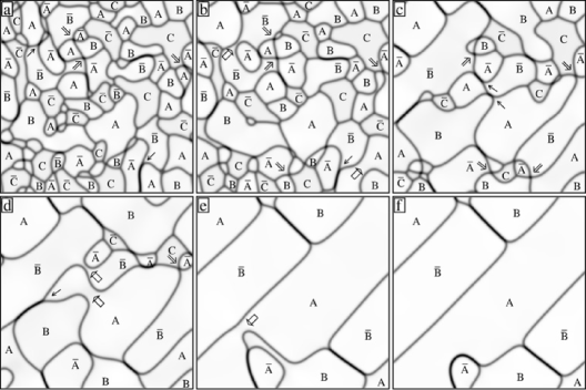
FIG. 1.: Temporal evolution of the extended–range-interaction model 5 under the phase transformation A1$\to$L1₀ shown in the $\eta^{2}$-representation for the simulation box size $V_{b}=128^{2}\times 1$ at $c=0.5$, the reduced temperature $T^{\prime}=T/T_{c}=0.7$, $|\varepsilon_{m}|=0.1$ and the following values of the reduced time $t^{\prime}=t\gamma_{ij}$: (a) 10; (b) 20; (c) 50; (d) 100; (e) 250; and (f) 280. The symbol A, $\overline{{\rm A}}$, B, $\overline{\rm B}$, C or $\overline{\rm C}$ indicates the type of the ordered domain as described in the text. The single, the double and the thick arrow indicates the splitting APB process, the quadruple junction of APDs, and the fusion-of-domain process, respectively, mentioned in the text.

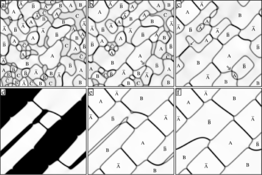
FIG. 2.: As figure 1, but at $|\varepsilon_{m}|=0.15$ and the following values of $t^{\prime}$: (a) 10; (b) 20; (c) 50; (d) 150; (e) 172; and (f) 350. Frame 2d is shown in the $\eta_{2}^{2}$-representation described in the text.

Figures 1–5 illustrate quasi-2D simulations for which microstructures include only the edge-on APBs normal to the (001) plane. The above-mentioned elimination of the volume-dependent elastic energy in such geometry is possible only for the (100) and (010)-ordered APDs A or $\overline{\rm A}$ and B or $\overline{\rm B}$ separated by the (110)-oriented flip-APB, while in the (001)-oriented domains C and $\overline{\rm C}$ this elastic energy is always present. Therefore, the tweed stage (ii) in these simulations corresponds to both the predominance of (110)-oriented APBs and the decrease of the number of domains C and $\overline{\rm C}$ in the microstructures.

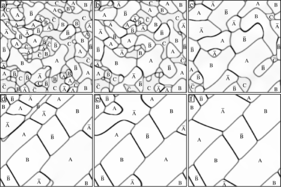
FIG. 3.: As figure 2, but for the intermediate-range-interaction model 4 at $T^{\prime}=0.67$ and the following values of $t^{\prime}$: (a) 10; (b) 20; (c) 50; (d) 170; (e) 200; and (f) 700.

Let us first consider figures 1–3 in which frames 1a–1b, 2a and 3a correspond to the initial stage; frames 1c–1d, 2b–2c, and 3b–3c, to the tweed stage; and the rest frames, to the twin stage. At both the initial and the tweed stage we can observe the following features of evolution [21]:

(a) The presence of abundant processes of fusion of in-phase domains which are one of the main mechanisms of domain growth at these stages.

(b) The presence of peculiar long-living configurations, the quadruple junctions of APDs (4-junctions) of the type A₁A₂$\overline{\rm A_{1}}$A₃ where A₂ and A₃ can correspond to any two of four types of APD different from A₁ and $\overline{\rm A_{1}}$.

(c) The presence of many processes of “splitting” of a shift-APB into two flip-APBs which is finished by either a fusion of in-phase domains mentioned in point (a) ($s\to f$ process), or a formation of a 4-junction mentioned in point (b) ($s\to 4j$ process).

For example, $s\to f$ processes can be followed in frames 1a–1b; 1c–1d; 1d–1e; 2c–2d; etc. The fusion with the disappearance of an intermediate APD which initially separates two in-phase domains to be fused [21] can be seen in the lower right part of frames 1a–1b. Several long-living 4-junctions are seen in frames 1a–1d and 2c–2d; and an $s\to 4j$ process can be followed in the lower right part of frames 1a–1c. Let us also note that the microstructural features (b) and (c) can be naturally explained by a significant excess of the surface energy of shift-APBs with respect to flip-APBs found in our CFM calculations for the systems under consideration.

Frames 3a–3c also display some (100)-oriented and thin “conservative” APBs [11, 21]. Such APBs are most typical of the short-range-interaction systems—see [11] and figure 4 below—where they have a low surface energy (being zero for the nearest-neighbor interaction model). Under an increase of the interaction range (as well as temperature or the deviation from stoichiometric composition $\delta c=0.5-c$) the anisotropy of this surface energy decreases, and so for model 4 such APBs are few, while for the extended-range-interaction model 5 they are absent at all.

Frames 1c–1d, 2b–2c, and 3b–3c (as well as 4a–4b) illustrate a (110)-type alignment of APBs between APDs A or $\overline{\rm A}$ and B or $\overline{\rm B}$ and a “dying out” of APDs C and $\overline{\rm C}$ at the tweed stage. Frames 1c and 1d also show that in the simulation with a realistic distortion parameter $|\varepsilon_{m}|=0.1$ (fitted to the structural data for CoPt) the APD size $l_{0}$ (20) characteristic of the tweed stage is about $(20-40)\,a$. It agrees with the order of magnitude of $l_{0}$ observed in the CoPt-type alloys FePt and FePd [27, 28].

Discussing the final, twin stage of the evolution we first mention some characteristic configurations observed in experimental studies of transient twinned microstructures [4, 27, 28, 29, 30]:

(1) “semi-loop” shift-APBs adjacent to the twin band boundaries;

(2) “S-shaped” shift-APBs stretching across the twin band;

(3) short and narrow twin bands—usually with one or two shift-APBs near their edges–lying within the main twin bands;

(4) an alignment of shift-APBs in the final, “nearly equilibrium” twin bands: within a (100) oriented band in a (110)-type polytwin the APBs tend to align normally to some direction ${\bf n}=(\cos\alpha,\sin\alpha,0)$ with a “tilting” angle $\alpha$ which is less than $\pi/4$ in CoPt and is close to zero in CuAu [29, 30].

Comparing our results with experiments one should consider that due to the limited size of the simulation box the twin band width $d$ in our simulations has the same order of magnitude as the APD size $l_{0}$ (20) characteristic of the tweed stage, while in experiments $d$ usually much exceeds $l_{0}$ [27, 28, 29, 30]. Therefore, the distribution of shift-APBs within twin bands in our simulation is usually much more close to equilibrium than in experiments. In spite of this difference, the simulations reproduce not only “nearly equilibrium” configurations (4) but also transient configurations (1)–(3) and elucidate their formation mechanisms. In particular, both the “semi-loop” and “S-shaped” shift-APBs are formed from regular-shaped approximately quadrangular APDs (characteristic of early twin stages) due to the disappearance of adjacent APDs which are “wrongly-oriented” with respect to the given twin band; it is seen, for example, in frames 1d–1f, 2e–2f, 3c–3e, etc. The formation of short and narrow twin bands with the edges touched by shift-APBs is illustrated by frame 2d (which is strikingly similar to the experimental microstructure shown in Fig. 2 of Ref. [4]) and also by frame 3d.

The alignment of shift-APBs mentioned in point (4) is illustrated by frames 2f and 3f, as well as 4d and 5a–5d. These frames show that the tilting angle $\alpha$ sharply depends on the interaction type, particularly on the interaction range, as well as on the concentration $c$ and temperature $T$. In particular, for the extended-range-interaction model 5 this angle is close to $\pi/4$; for the intermediate-range-interaction model 4 (which seems to more realistically describe properties of CoPt-type alloys) the angle $\alpha$ is less than $\pi/4$, i.e. APB planes are tilted to the tetragonality axis; and for the short-range-interaction models 1 and 2 the APB planes tend to be parallel with the tetragonality axis, i. e. $\alpha\simeq 0$. Such interaction-dependent alignment of shift-APBs can be explained [20] by the competition between the anisotropy of their surface energy — which for both the intermediate and short-ranged-interaction systems tends to orient APBs parallel with the tetragonality axis decreasing the angle $\alpha$, and a tendency to minimize the APB area within the given twin band which corresponds to $\alpha=\pi/4$. Therefore, the comparison of experimental tilting angles with the theoretical calculations [20] can provide both qualitative and quantitative information about the interatomic interactions in an alloy.

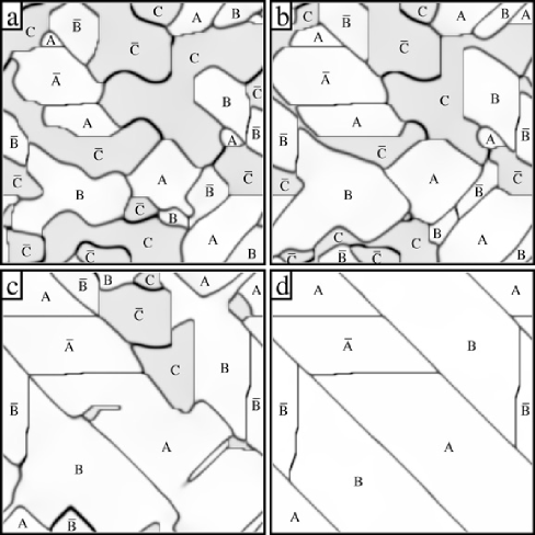
FIG. 4.: As figure 2 but for the short-range-interaction model 1 at $T^{\prime}=0.9$ and the following values of $t^{\prime}$: (a) 30; (b) 40; (c) 60; and (d) 120.

Figure 4 illustrates evolution for model 1 which describes the short-ranged-interaction systems such as alloys Cu–Au [11]. The microstructures for such systems include many conservative APBs mentioned above, and the shift-APBs in the final frame 4d are “step-like” consisting of (100)-type oriented conservative segments and small non-conservative ledges (being similar to the APBs observed in the L1₂-ordered Cu₃Au alloy [11]). These step-like APBs can be viewed as a “facetted” version of tilted APBs seen in frames 2f, 3f, 5c and 5d. As mentioned, under an increase of temperature $T$ or “non-stoichiometry” $\delta c=0.5-c$ the anisotropy in the APB energy rapidly decreases. It results in sharp, phase-transition-like changes in morphology of aligned APBs, from the “faceting” to the “tilting”, which is illustrated by frames 5a–5d. These morphological changes are realized via some local bends of facetted APBs illustrated by frames 5a–5b. Therefore, this “morphological phase transition” is actually smeared over some intervals of temperature or concentration, but frames 5a–5d show that these intervals can be relatively narrow.

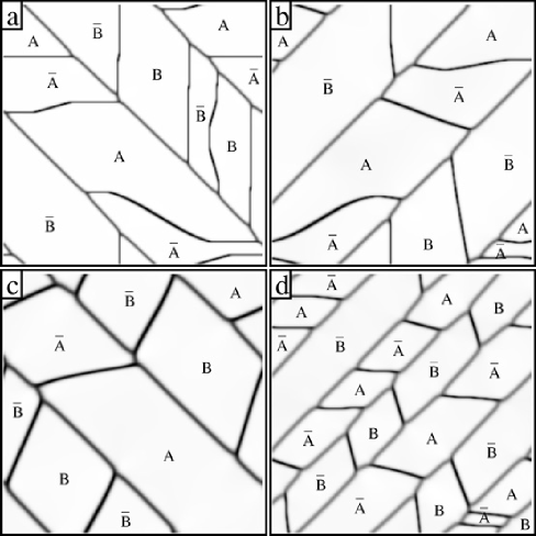
FIG. 5.: As figure 1 but for model $2$ at $|\varepsilon_{m}|=0.1$ and the following values of $c$, $T^{\prime}$ and $t^{\prime}$: (a) $c=0.5$, $T^{\prime}=0.77$, $t^{\prime}=350$; (b) $c=0.46$, $T^{\prime}=0.77$, $t^{\prime}=350$; (c) $c=0.5$, $T^{\prime}=0.95$, $t^{\prime}=300$; and (d) $c=0.44$, $T^{\prime}=0.77$, $t^{\prime}=300$.

Finally, let us make a general remark about the kinetics of multivariant orderings in alloys, such as the D0₃, L1₂ and L1₀ orderings considered in Refs. [11, 19, 20, 21] and in this work. It is well known that the thermodynamic behavior of different systems under various phase transitions reveals features of universality and insensitivity to microscopical details of structure, particularly in the critical region near thermodynamic instability points. The results of this and other studies of multivariant oderings show that such universality does not seem to hold for their phase transformation kinetics, anyway outside the critical region (which for such orderings is usually either quite narrow or absent at all). The microstructural evolution reveals a great variety of peculiar features, the detailed form of which sharply depends on the type of interatomic interaction, structure, the degree of deviation from stoichiometric composition, and other “non-universal” characteristics.

REFERENCES

- [1] Present address: Ames Laboratory, Ames, Iowa 50011, USA.
- [2] C. Frontera et al., Phys. Rev. B 55, 212 (1997).
- [3] A. G. Khachaturyan, Theory of Structural Phase Transformations in Solids ( Wiley, New York, 1983).
- [4] L.-Q. Chen,Y. Wang and A. G. Khachaturyan, Phil. Mag. Lett. 65, 15 (1992).
- [5] A. G. Khachaturyan, in Phase Transformations and Evolution in Materials, edited by P. Turchi and A. Gonis (TMS, Warrendale, 2000), 3-18, and references therein.
- [6] G. Martin, Phys. Rev. B 41, 2279 (1990).
- [7] V. G. Vaks and S. V. Beiden, Sov. Phys.–JETP 78, 546 (1994).
- [8] V. G. Vaks, S. V. Beiden and V. Yu. Dobretsov, JETP Lett. 61, 68 (1995).
- [9] V. G. Vaks, JETP Lett. 63, 471 (1996).
- [10] K. D. Belashchenko and V. G. Vaks, J. Phys.: Cond. Matter 10, 1965 (1998).
- [11] K. D. Belashchenko et al., J. Phys.: Cond. Matter 11, 10593 (1999).
- [12] K. D. Belashchenko et al., in Phase Transformations and Evolution in Materials, edited by P. Turchi and A. Gonis (TMS, Warrendale, 2000), 139-158.
- [13] M. Nastar, V. Yu. Dobretsov and G. Martin, Phil. Mag. A 80, 155 (2000).
- [14] V. Yu. Dobretsov et al., Europhys. Lett. 31, 417 (1995).
- [15] V. Yu. Dobretsov, V. G. Vaks and G. Martin, Phys. Rev. B 54, 3227 (1996).
- [16] K. D. Belashchenko and V. G. Vaks, Phys. Lett. A 222, 345 (1996).
- [17] K. D. Belashchenko and V. G. Vaks, Sov. Phys.–JETP 85, 390 (1997).
- [18] V. Yu. Dobretsov and V. G. Vaks, J. Phys.: Cond. Matter 10, 2261 and 2275 (1998).
- [19] K. D. Belashchenko, G. D. Samolyuk and V. G. Vaks, J. Phys.: Cond. Matter 11, 10567 (1999).
- [20] V. G. Vaks, JETP Lett. 73, 237 (2001).
- [21] I. R. Pankratov and V. G. Vaks, 13, (2001), in press.
- [22] R. Kikuchi, Phys. Rev. 81 988 (1951).
- [23] A. Finel, in Statics and Dynamics of Alloy Phase Transformations (NATO ASI Series B, 319), edited by A. Gonis and P. Turchi ( Plenum, N.-Y., 1994), 495-540.
- [24] V. G. Vaks and G. D. Samolyuk, Sov. Phys.–JETP 88, 89 (1999).
- [25] F. Chassagne et al., Acta Met. 37, 2329 (1989).
- [26] Y. Tanaka et al., Phil. Mag. A 69, 925 (1994).
- [27] B. Zhang, M. Lelovic and W. A. Soffa, Scripta Met. 25, 1577 (1991).
- [28] C. Yanar, J. Wiezorek and W. A. Soffa, in Phase Transformations and Evolution in Materials, edited by P. Turchi and A. Gonis (TMS, Warrendale, 2000), 39-54.
- [29] C. Leroux et al., Phil. Mag. B 64, 57 (1991)
- [30] M. Guymont and J. Bonneaux, Scripta Met. 36, 1175 (1997).