The 3-SAT problem with large number of clauses in the $\infty$-replica symmetry breaking scheme

Abstract

In this paper we analyze the structure of the UNSAT-phase of the over-constrained $3$-SAT model by studying the low temperature phase of the associated disordered spin model. We derived the full Replica Symmetry Breaking (RSB) equations for a general class of disordered spin models which includes the Sherrington-Kirkpatrick (SK) model, the Ising $p$-spin model as well as the over-constrained $3$-SAT model as particular cases. We have numerically solved the $\infty$-RSB equations using a pseudo-spectral code down to and including zero temperature. We find that the UNSAT-phase of the over-constrained $3$-SAT is of the $\infty$-RSB kind: in order to get a stable solution the replica symmetry has to be broken in a continuous way, similarly to the SK model in external magnetic field.

1 Introduction

A combinatorial optimization problem is defined, in a broad sense, by specifying a certain number of free variables constituting it and the conditions that its solution must satisfy. In treating an optimization problem the fundamental step is to find the most efficient algorithm yielding the solution. Efficient from the point of view of all the computing resources needed for its performance, the most important of which is the time requirement, and, in particular, its dependence on the size of the problem. By size we mean, in an informal way, the number of variables, or, even, the number of conditions.

A computational hard problem [1, 2] is an optimization problem for which the time needed to find the solution, or to determine with certainty that it has no solution, very sensitively increases with the size. More specifically there are no polynomial algorithms able to solve it. This kind of problems are therefore called intractable or Non Polynomial (NP).

Any NP problem can be reduced to a particular NP paradigmatic problem (the SAT problem) exploiting algorithms performing such a mapping in a polynomial time [3, 4]. Computer scientists call this class of very hard combinatorial optimization problems the class of Non Polynomial-Complete (NPC) problems [1].

Summing-up, a NPC problem is defined, in a qualitative way, as an optimization problem whose solutions, or the certainty that it has no solution, can only be found, in the worst case, by algorithms whose computation time grows faster than any polynomial with the number of variables of the system.

In this paper we shall consider the 3-SAT problem [4]. This is a particular version of SAT problem, which is the paradigm of NPC combinatorial problems showing a phase transition. For this problem the free variables are boolean variables and the conditions are sets of three boolean numbers. Its importance, apart from being a historical one, comes from the fact that even if theoretically any NPC problem can be mapped in any other, in practice given problems are better suited for proving such correspondence. Of these reference problems one of the most useful (and used) is the 3-SAT.

In the last years a one to one correspondence has been observed between computational hard problems and the ground state properties of spin-glass models [5, 6]. Statistical mechanics has been applied to the study of universal behaviour in the computational cost of some class of algorithms, searching for solutions of random realizations of the prototype of the NPC problems: the Satisfaction (SAT) problem [7]. The investigation of the properties of NPC problems is then performed through the introduction of an energy or cost function and an artificial temperature. In this mapping the actual NPC problem is recovered as the $T=0$ limit of the associated statistical mechanical problem. Such an approach has been implemented both numerically, using simulated annealing algorithms [8]), and analytically.

To set up a statistical mechanical approach one first introduces a semidefinite positive Hamiltonian ${\cal{H}}[C]$ function, defined for each given instance $C$ of the problem, constructed in such a way that if the configuration $C^{*}$ is solution of the computational problem then ${\cal{H}}[C^{*}]=0$. On the contrary, if ${\cal{H}}[C]>0$ for any $C$ then problem does not admit solution. Having defined an Hamiltonian, the associated statistical mechanical problem is described by the partition function

$$Z(\beta)=\sum_{C}\exp(-\beta\cal{H}[C])\ ,$$ (1)

where $\beta^{-1}=T$ is the (artificial) temperature of the system. Proceeding further one introduces the usual thermodynamic quantities, e.g., the energy

$$U(\beta)=-{\partial\ln(Z(\beta))\over\partial\beta}\ .$$ (2)

The mapping is not trivial since intensive quantities, such as the energy density $u\equiv U/N$, do not depend on $N$ in the infinite $N$ limit, so that a computation of their average over the distribution of instances of the computational problem is sufficient to obtain relevant informations on its satisfiability.

Eventually, to recover the original computational problem, the limit $T\to 0$ has to be taken. We stress that, in this approach, the temperature only plays a role for the constsruction of a statistical mechanics problem, of which the only interesting features are those at $T=0$.

In this approach, phase transition concepts play an important role to build a theory for typical case complexity in theoretical computational science. The importance comes from the fact that NPC decision problems, that are computationally hard in the worst case, may be not in the typical case, if one excludes the critical regions of the parameter space, where almost all instances become computationally hard to solve. The computational critical region corresponds to a phase transition region in statistical mechanics language. Far from phase boundaries the problems are either under-constrained or over-constrained and one can determine search procedures able to find solutions, or certainty of no solution, in polynomial times: the results of worst-case complexity theory are not very relevant in practice and what is necessary is a theory for typical-case complexity. To such a purpose, the analysis of general search methods applied to different classes of hard computational problems, characterized by a large number or relevant, randomly generated, variables, is fundamental.

Variables are under-constrained when the minimal number of violated clauses does not depend on their possible assignments. In particular this is true when they do not appear in any clause. In the under-constrained phase the clauses of the problem can always be satisfied (SAT phase). On the contrary, variables are over-constrained when they cannot satisfy simultaneously all the clauses imposed on them. In this case we are in the UNSAT phase. Going back to the mapping onto a statistical mechanical problem, the UNSAT-phase corresponds to a frozen (spin-glass) phase while the SAT-phase corresponds to an ordered (ferromagnetic) phase.

The 3-SAT problem, and, in general, the $K$-SAT problem where the clauses contain a number $K$ of elements, can be mapped onto a diluted long-range spin-glass model [5, 6]. The model is mean-field because of the lack of geometrical correlations in the clauses. However, since each spin has only a finite number of neighbours strong local field fluctuations, stronger than in those of fully connected spin-glass, are present.

The relevant parameter driving the SAT/UNSAT transition is the ratio $\alpha$ between clauses and number of variables of the system, which is the connectivity in the statistical mechanical analogue of the combinatorial problem.

Indeed too many conditions cause the unsatisfiability of the problem. The entropy of the associated spin model gives a measure of the typical number of solutions. Therefore at the transition an abrupt disappearance of all (exponentially numerous) solutions makes the entropy jump to zero.

For $K=1$ and $2$ the problem is solvable: the time to find the solutions grows polynomially (actually even linearly [3]) with the number of variables. For $K\geq 3$ the problem is, on the contrary, NPC. The transition threshold for 3-SAT has been determined numerically at $\alpha_{c}(3)\simeq 4.25-4.30$ [9].

Based on the mapping of random clauses onto the quenched disorder of the associated spin model, in Ref. [5, 6] the Replica trick was introduced to compute the statistical mechanics of the K-SAT problem and the Replica Symmetric (RS) theory was carried out. The K-SAT problem is naturally mapped onto a disordered spin model with finite connectivity, where the role of connectivity is played by the density of clauses. Even if it gives a qualitative good pattern of the transition it is, however, unable to predict correctly the value of the transition threshold between the SAT-phase and the UNSAT-phase and the correct thermodynamic quantities in the UNSAT-phase.

The failure of the RS solution can be traced back to the existence of a very large number of equilibrium states of the associated statistical mechanical problem in the thermodynamic limit $N\to\infty$. To deal with those, and improve the knowledge of the structure of the solutions of the decision problem, it is necessary to break the Replica Symmetry. Replica Symmetry Breaking (RSB) in diluted models is a very hard issue, due to the complex structure of the saddle point equations, for recent approaches see [10, 11].

As shown in [12] the SAT/UNSAT transition results from the sudden freezing of a finite number of variables, as $\alpha$ increases above $\alpha_{c}$. These variables form a backbone that does not disappear in the thermodynamic limit. Information about the structure of this backbone and about the mutual overlap between different assignments minimizing the cost function in the UNSAT phase is, then, very important to understand the transition.

In an attempt to overcome the difficulty of solving a spin glass diluted model a variational approach, both for RS and $1$-RSB solution, has been recently proposed. It is based on the existence of the backbone of over-constrained variable that remains finite in the thermodynamic limit [13]. This circumvent the necessity of solving the self-consistent equations for RS and $1$-RSB, but does not resolve the question about the nature of the RSB solution in the UNSAT-phase. Thus the relation between RSB transition and the typical case complexity theory is yet an open question.

In order to investigate the the nature of the RSB solution in the UNSAT-phase, in this paper we shall consider the K-SAT problem with $K=3$, the simplest NPC problem of this class, in the limit of a large number of clauses $\alpha\gg 1$ (over-constrained), where the associated statistical mechanical problem can be handled with known techniques of disordered spin systems. The basic idea is that since there should be no other transitions for $\alpha>\alpha_{c}$, the structure of the UNSAT-phase for $\alpha\gg\alpha_{c}$ should be representative of the whole UNSAT-phase in the range $\alpha>\alpha_{c}$. Performing a careful study of the thermodynamic quantities down to zero temperature of the associated disordered spin model we find that the RSB is infinitely broken ($\infty$-RSB) in the UNSAT-phase.

Moreover, using the first two terms in the asymptotic expansion in $1/\sqrt{\alpha}$ of the thermodynamic quantities, we can obtain an upper bound for $\alpha_{c}$.

The paper is organized as follows. In Section 2 we introduce the model. The details of the derivation of the $\infty$-RSB solution with an arbitrary gauge are given in section 4. The calculation is carried out for a general model introduced in Section 3, to which the over-constrained $3$-SAT problem belongs. Here we also sketch the procedure used for the numerical of solution of the $\infty$-RSB solution. The $\infty$-RSB solution for the over-constrained $3$-SAT model is discussed in Sections 5 and 6.

2 The over-constrained 3-SAT model

The model we study has been introduced in [14], where the analysis of RSB at one and two steps has been carried out. The $3$-SAT model is defined by a set of boolean variables $s(i)=0,1$, defined on the sites $i=1,\ldots,N$, and an ensemble of randomly generated $3$-SAT boolean formulae. First the random boolean formulae are constructed by assign to each triplet $\{i_{1},i_{2},i_{3}\}$, with $i_{1}<i_{2}<i_{3}$, a set of three independent variables $\epsilon_{1,2,3}$ which take the value $+1$ or $-1$ with probability $1/2$. Next for each instance of the problem triplets of randomly chosen sites $\{i_{1},i_{2},i_{3}\}$ are selected by assigning to the variables $r_{i_{1},i_{2},i_{3}}$ the value $1$ with probability $p\equiv\alpha N^{-2}$ and $0$ with probability $1-p$. For $N\to\infty$ there are $\alpha N$ variables $r$ which are different from zero, and hence $\alpha N$ $3$-SAT boolean formulae..

If we introduce the spin variables $\sigma(i)=1-2s(i)$, the cost function reads

$${\cal{H}}=\sum_{i_{1}<i_{2}<i_{3}}r_{i_{1},i_{2},i_{3}}\frac{1-\epsilon_{1}^{(i_{1},i_{2},i_{3})}\sigma(i_{1})}{2}\frac{1-\epsilon_{2}^{(i_{1},i_{2},i_{3})}\sigma(i_{2})}{2}\frac{1-\epsilon_{3}^{(i_{i},i_{2},i_{3})}\sigma(i_{3})}{2}.$$ (3)

which is nothing but the number of unsatisfied clauses. Indeed it is easy to see that each term is either $1$ (unsatisfied) or $0$ (satisfied). Note that ${\cal{H}}=0$ if and only if all the clauses are satisfied.

The statistical mechanical approach to the $3$-SAT problem takes ${\cal{H}}$ as the Hamiltonian of a disordered spin system, and, as discussed above, studies the properties of the ground state.

The fundamental quantities in studying the hard optimization problems with the tools of statistical mechanics are the zero temperature energy and entropy densities, respectively $u_{0}$ and $s_{0}$, in the thermodynamic limit. $u_{0}$ represents the average over the distribution of clauses of the number of clauses that are not satisfied by the formula (3). $s_{0}$ is the logarithm of the number of solutions satisfying the formula divided by the number of variables. For the behaviour of these quantities as functions of the connectivity-like parameter $\alpha$, the conjecture is done[5, 6] that

$$u_{0}(\alpha)=0\ , \hskip 28.45274pts_{0}(\alpha)>0,\hskip 56.9055pt\mbox{for $\alpha<\alpha_{c}$}$$ (4)

$$u_{0}(\alpha)>0\ , \hskip 28.45274pts_{0}(\alpha)=0,\hskip 56.9055pt\mbox{for $\alpha>\alpha_{c}$}$$ (5)

For $\alpha\ll\alpha_{c}$ the problem is quite under-constrained and it is relatively easy to find an assignment of variables $\sigma_{i}$ satisfying the clauses. In other words for $\alpha<\alpha_{c}$ the problem is SAT, with probability going to 1 for $N\to\infty$, On the contrary for $\alpha>\alpha_{c}$ the problem does not have solutions, UNSAT-phase. The analysis of the UNSAT-phase is in general rather hard. The most difficult case occurs around $\alpha_{c}$ where an exponential time may be needed to determine the unsatisfiability. Away from the critical region, i.e., $\alpha\gg\alpha_{c}$, to prove unsatisfiability is easier, and more insight into the structure of the phase space can be gained.

In the present paper we will work in the over-constrained approximation $\alpha\gg\alpha_{c}$, where the computation strongly simplifies. This limit is obtained by expanding in $1/\sqrt{\alpha}$ to second order, after having rescaled the temperature $\beta\to\beta/\sqrt{\alpha}$ . For further details See [14].

Note that in Ref. [14] the reduced inverse temperature was $\beta=\mu/\sqrt{\alpha}$. Here we will, instead, keep the notation $\beta$ also for the reduced inverse temperature. Moreover in [14] the clauses are erroneously over counted in the evaluation of the partition function [15]. This, however, does not produce any relevant change, apart from a rescaling of the reduced temperature and of the energy and the free energy of a factor $1/\sqrt{6}$, leaving the entropy invariant. In order to make a comparison with the results shown there, it is enough to multiply $\beta$, the free energy and the energy shown in the present paper by a factor $\sqrt{6}$.

3 The replica approach in a generalized form

The 3-SAT model belongs to the family of spin models interacting via quenched random couplings. These are described by a random Hamiltonian ${\cal H}[J;\sigma]$ where $J$ are the random “quenched” couplings. For example, in the Sherrington-Kirkpatrick (SK) model $J$ is a symmetric Gaussian matrix of zero mean and variance proportional to $1/N$ [16], while in its $p$-spin generalization the variance goes like $1/N^{p-1}$ [17]. For the 3-SAT problem the disorder is introduced by the random clauses imposed on the set of variables. In the simple limit that we are considering here, the quenched disorder is represented by the random $\pm 1$ variables $\epsilon^{(i_{1},i_{2},i_{3})}$, assigning a clause on the three sites $i_{1}$, $i_{2}$ and $i_{3}$ [14].

For any fixed coupling realization $J$, the partition function of the spin system, with $N$ spins, is given by [18, 19]

$$Z_{N}[J]=\mbox{Tr}_{\sigma}\ \exp\bigl{(}-\beta{\cal H}[J;\sigma]\bigr{)}$$ (6)

and the quenched free energy per spin is

$$f_{N}=-{1\over N\beta}\ \overline{\,\ln Z_{N}\,}=-{1\over N\beta}\ \int d[J]\ P[J]\ \ln Z_{N}[J]$$ (7)

where $\overline{(\cdots)}$ indicates the average over the couplings realizations. We assume that the thermodynamic limit of the free energy, $-\lim_{N\to\infty}\ln Z_{N}[J]\ /\ N\beta$ is well defined and is equal to the quenched free energy $f=\lim_{N\to\infty}f_{N}$ for almost all coupling realizations $J$ (self-average property).

The analytic computation of the quenched free energy, i.e., of the average of the logarithm of the partition function, is a quite difficult problem, even in simple cases as nearest neighbour one dimensional models. However, since the integer moments of the partition function are easier to compute, the standard method uses the so called “replica trick” by considering the annealed free energy $f(n)$ of $n$ non-interacting ‘replicas’ of the system [16, 18, 19],

$$f(n)=-\lim_{N\to\infty}{1\over N\beta n}\ \ln\left[\overline{(Z_{N}[J])^{n}}\right].$$ (8)

The quenched free energy of the original system is then recovered as the continuation of $f(n)$ down to the unphysical limit $n=0$,

$$f=-\lim_{N\to\infty}\lim_{n\to 0}{\overline{(Z_{N}[J])^{n}}-1\over N\beta n}=\lim_{n\to 0}f(n).$$ (9)

In the last equality we assumed that the replica limit and the thermodynamic limit can be exchanged. This procedure replaces the original interactions in the real space with couplings among different replicas. The interested reader can find a complete and detailed presentation of the replica method for disordered statistical mechanical systems in Ref. [19] and in Ref. [18].

In what follows we shall consider disordered spin systems for which $f$ in the replica space can be written in the form

$$\beta f\left[Q_{ab},\Lambda_{ab}\right]=\beta f_{0}(\beta)-\frac{\beta^{2}}{2}\lim_{n\to 0}\frac{1}{n}\sum_{a\neq b}^{1,n}g\left(Q_{ab}\right)+\frac{\beta^{2}}{2}\lim_{n\to 0}\frac{1}{n}\sum_{a\neq b}^{1,n}\Lambda_{ab}Q_{ab}$$

$$\hbox to0.0pt{\hss${}-{}$}\lim_{n\to 0}\frac{1}{n}\log\mbox{Tr}_{\sigma}\exp\left(\frac{\beta^{2}}{2}\sum_{a\neq b}\Lambda_{ab}\,\sigma^{a}\sigma^{b}\right)$$ (10)

where $Q_{ab}$ is the spin-overlap matrix in the replica space between replicas $a$ and $b$:

$$Q_{ab}=\frac{1}{N}\sum_{i=1}^{N}\,\overline{\langle\sigma_{i}^{a}\,\sigma_{i}^{b}\rangle}$$ (11)

and $\Lambda_{ab}$, the Lagrange multiplier associated with $Q_{ab}$, gives the interaction matrix between spins of different replicas. Angular brackets denote thermal average. Stationarity of $f$ with respect to variations of $\Lambda_{ab}$ and $Q_{ab}$ leads to the self-consistency equations for the matrices $\Lambda$ and $Q$:

$$\Lambda_{ab} = g_{1}\left(Q_{ab}\right)$$ (12)

$$Q_{ab} = \frac{\mbox{Tr}_{\sigma}\ \sigma^{a}\sigma^{b}\exp\left(\frac{\beta^{2}}{2}\sum_{a\neq b}\Lambda_{ab}\sigma^{a}\sigma^{b}\right)}{\mbox{Tr}_{\sigma}\exp\left(\frac{\beta^{2}}{2}\sum_{a\neq b}\Lambda_{ab}\sigma^{a}\sigma^{b}\right)}$$ (13)

where we have used the short-hand notation

$$g_{n}(z)\equiv\frac{d^{n}g(z)}{dz^{n}}\qquad n=1,2,\ldots$$ (14)

The function $g$ and the constant $f_{0}$ depend on the specific model. For example for the SK model we have[16]:

$$g(z)=\frac{z^{2}}{2},\hskip 28.45274ptf_{0}=-\frac{\beta}{4}.$$ (15)

Similarly the $p$-spin model [17] is recovered for

$$g(z)=\frac{z^{p}}{2},\hskip 28.45274ptf_{0}=-\frac{\beta}{4}\hskip 14.22636pt$$ (16)

Finally, for the $3$-SAT problem in the limit of low dilution we have [14]:

$$g(z)=\frac{1}{384}(1+z)^{3},\hskip 14.22636ptf_{0}=-\frac{\beta}{96}+\frac{\sqrt{\alpha}}{48}$$ (17)

In the following we will use $f_{0}=-\beta/96$, the only consequence being a shifting of the free energy density $f$ and of the internal energy density $u$ by a factor $\sqrt{\alpha}/48$.

4 Infinite Replica Symmetry Breaking Solution

4.1 $\infty$-RSB solution

To evaluate the $n\to 0$ limits in (10) one has to make an Ansatz on the structure of matrices $\Lambda$ and $Q$, i.e., to choose a Replica Symmetry Breaking (RSB) scheme. In order to be as general as possible, we shall use the RSB scheme introduced by de Dominicis, Gabay and Orland [20, 21], which besides the Edwards-Anderson order parameter [22] also involves the anomaly to the linear response function, also called Sompolinsky’s anomalies [23]. The more usual Parisi’s RSB scheme is recovered by a proper gauge fixing. Here we shall only report the main results, since the calculation is straightforward. The interested reader can find some details in Ref. [20, 21].

By applying the RSB scheme infinite times and introducing two functions $q(x)$ and $\lambda(x)$, $0\leq x\leq 1$, one for each matrix, the free energy functional (10) becomes [20, 21]:

$$\beta f(\beta)=\beta f_{0}(\beta)+\frac{\beta^{2}}{2}\left[g\left(q(1)\right)+\lambda(1)\left(1-q(1)\right)\right]+\frac{\beta}{2}\int_{0}^{1}dx\ g_{1}\left(q(x)\right)\dot{\Delta}_{q}(x)$$ (18)

$$-\frac{\beta}{2}\int_{0}^{1}dx\left[q(x)\dot{\Delta}_{\lambda}(x)+\lambda(x)\dot{\Delta}_{q}(x)\right]-\beta\int_{-\infty}^{+\infty}\frac{dy}{\sqrt{2\pi\lambda(0)}}\exp\left(-\frac{y^{2}}{2\lambda(0)}\right)\phi(0,y)$$

where $\phi(0,y)$ is the solution evaluated at $x=0$ of the the Parisi’s equation

$$\dot{\phi}(x,y)=-\frac{\dot{\lambda}(x)}{2}\,\phi^{\prime\prime}(x,y)+\frac{\dot{\Delta}_{\lambda}(x)}{2}\,\phi^{\prime}(x,y)^{2}$$ (19)

with the boundary condition

$$\phi(1,y)=T\log\left(2\cosh\beta y\right)$$ (20)

and $\Delta_{q}(x)$ and $\Delta_{\lambda}(x)$ are the anomalies associated with the order parameters $q(x)$ and $\lambda(x)$. We have used the standard notation and denote derivatives with respect to $x$ by a dot and derivatives with respect to $y$ by a prime. Note that with this notation Sompolinsky’s $\Delta^{\prime}$ becomes $T\dot{\Delta}$. It is easy to see that using (15) one recovers the Sompolinsky functional for the SK model [23], and inserting the Parisi’s gauge $\dot{\Delta}_{q}(x)=-\beta x\dot{q}(x)$ the Parisi’s functional [24].

The Parisi’s equation (19) can be included into the free energy via the Lagrange multiplier $P(x,y)$ and the initial condition at $x=1$ (20) via $P(1,y)$. The free energy then becomes [25]

$$\beta f_{v}(\beta)=\beta f(\beta)+\beta\int_{-\infty}^{+\infty}dy\ P(1,y)\,\bigl{[}\phi(1,y)-T\log\left(2\cosh\beta y\right)\bigr{]}$$ (21)

$$\hbox to0.0pt{\hss${}-{}$}\beta\int_{0}^{1}dx\int_{-\infty}^{+\infty}dy\ P(x,y)\left[\dot{\phi}(x,y)+\frac{\dot{\lambda}(x)}{2}\phi^{\prime\prime}(x,y)-\frac{\dot{\Delta}_{\lambda}(x)}{2}\left(\phi^{\prime}(x,y)\right)^{2}\right].$$

By this construction $f_{v}$ is stationary with respect to variations of $P(x,y)$, $P(1,y)$, $\phi(x,y)$, $\phi(0,y)$, the order parameters $q(x)$ and $\lambda(x)$ and anomalies $\dot{\Delta}_{q}(x)$ and $\dot{\Delta}_{\lambda}(x)$. Variations with respect to $P(x,y)$ and $P(1,y)$ simply give back eqs. (19) and (20). Stationarity with respect to variations of $\phi(x,y)$ and $\phi(0,y)$ leads to a partial differential equation for $P(x,y)$:

$$\dot{P}(x,y)=\frac{\dot{\lambda}(x)}{2}\,P^{\prime\prime}(x,y)+\dot{\Delta}_{\lambda}(x)\,\bigl{[}P(x,y)\,\phi^{\prime}(x,y)\bigr{]}^{\prime}.$$ (22)

with the boundary condition at $x=0$

$$P(0,y)=\int_{-\infty}^{+\infty}\frac{dy}{\sqrt{2\pi\lambda(0)}}\exp\left(-\frac{y^{2}}{2\lambda(0)}\right).$$ (23)

Finally, variations of $q(x)$, $\dot{\Delta}_{q}(x)$, $\lambda(x)$ and $\dot{\Delta}_{\lambda}(x)$ lead to

$$\dot{\Delta}_{\lambda}(x)=g_{2}\left(q(x)\right)\dot{\Delta}_{q}(x)$$ (24)

$$\lambda(x)=g_{1}\left(q(x)\right)$$ (25)

$$\Delta_{q}(x)=-\beta\bigl{[}1-q(1)\bigr{]}+\int_{-\infty}^{\infty}dy\,P(x,y)\,\phi^{\prime\prime}(x,y)$$ (26)

$$q(x)=\int_{-\infty}^{\infty}dy\,P(x,y)\,\phi^{\prime}(x,y)^{2}$$ (27)

with $\Delta_{q}(1)=0$, the anomalies at the shortest time-scale, corresponding to $x=1$, being zero by construction.

The Lagrange multiplier $P(x,y)$ gives the probability distribution of local fields. One may indeed associate a given overlap $q(x)$ with a time scale $\tau_{x}$ such that for times of order $\tau_{x}$ states with an overlap equal to $q(x)$ or greater can be reached by the system. In this picture the $P(x,y)$ becomes the probability distribution of frozen local fields $y$ at the time scale labeled by $x$ [25].

By partial derivate the above expressions we can obtain some useful relations. For example, deriving with respect to $x$ equations (27) and (25), or equivalently (26) and (24), one gets

$$g_{2}\left(q(x)\right)\int_{-\infty}^{\infty}dy\ P(x,y)\ \phi^{\prime\prime}(x,y)^{2}=1.$$ (28)

A further derivation with respect to $x$ leads to

$$g_{3}\bigl{(}q(x)\bigr{)}\,\dot{q}(x)+g_{2}\bigl{(}q(x)\bigr{)}\int^{\infty}_{-\infty}dy\,P(x,y)\,\bigl{[}\dot{\lambda}(x)\,\phi^{\prime\prime\prime}(x,y)^{2}+2\dot{\Delta}_{\lambda}(x)\,\phi^{\prime\prime}(x,y)^{3}\bigr{]}=0.$$ (29)

Using equations (25) and (24) this becomes

$$\hbox to0.0pt{\hss${}-{}$}\frac{\dot{q}(x)}{\dot{\Delta}_{q}(x)}=-\frac{\dot{\lambda}(x)}{\dot{\Delta}_{\lambda}(x)}=\frac{2\int dy^{\infty}_{-\infty}P(x,y)\ \phi^{\prime\prime}(x,y)^{3}}{g_{3}\left(q(x)\right)+g_{2}\left(q(x)\right)\int^{\infty}_{-\infty}dyP(x,y)\ \phi^{\prime\prime\prime}(x,y)^{2}},$$ (30)

which determines the gauge relation between $q(x)$ and $\Delta_{q}(x)$ and between $\lambda(x)$ and $\Delta_{\lambda}(x)$, the Parisi’s $\beta x$.

Finally we note that from eq. (27) and the interpretation of $P(x,y)$ distribution of local fields, $m(x,y)=\phi^{\prime}(x,y)$ can be interpreted as the local magnetization over the time-scale $x$. It obeys the equation

$$\dot{m}(x,y)=-\frac{\dot{\lambda}(x)}{2}\,m^{\prime\prime}(x,y)+\dot{\Delta}_{\lambda}(x)\,m(x,y)\ m^{\prime}(x,y)\ ,$$ (31)

with initial condition

$$m(1,y)=\tanh(\beta y).$$ (32)

In the next Section we shall report the results of numerical integration of the above equations for the specific case of $3$-SAT in the limit of a large number of clauses.

4.2 Thermodynamic quantities

Since the free energy density $f_{v}$ [eq. (21)] is stationary we can easily calculate thermodynamic derivatives to compute for example the the energy density $u$:

$$u=\frac{\partial}{\partial\beta}\,\beta f_{v}=\frac{\partial}{\partial\beta}\,\beta f_{0}+\beta\bigl{[}g\left(q(1)\right)+\lambda(1)\left(1-q(1)\right)\bigr{]}-\frac{1}{2}\int_{0}^{1}dx\ q(x)\ \dot{\Delta}_{\lambda}(x)$$ (33)

$$+\int_{-\infty}^{\infty}dy\ P(1,y)\ \phi(1,y)-\int_{-\infty}^{\infty}dy\ P(0,y)\ \phi(0,y)-\int_{-\infty}^{\infty}dy\ P(1,y)\ y\ \tanh(\beta y).$$

This expression can be simplified using the relation

$$\int_{-\infty}^{\infty}dy\ P(1,y)\ \phi(1,y)-\int_{-\infty}^{\infty}dy\ P(0,y)\ \phi(0,y)=-\frac{1}{2}\int_{0}^{1}dx\ q(x)\,\dot{\Delta}_{\lambda}(x)\ .$$ (34)

which follows computing $\int_{0}^{1}dx\int_{-\infty}^{\infty}dyP(x,y)\,\dot{\phi}(x,y)$ using either (19) or (22) and equating the results.

We can equivalently compute $u$ by taking the derivative of the free energy density (10) as a function of the generic matrix $Q_{ab}$, before any RSB scheme is introduced:

$$\frac{\partial}{\partial\beta}\,\beta f\left[Q_{ab},\Lambda_{ab}\right]=f_{0}(\beta)+\beta\frac{\partial}{\partial\beta}f_{0}(\beta)-\beta\lim_{n\to 0}\frac{1}{n}\sum_{a\neq b}^{1,n}g\left(Q_{ab}\right)$$ (35)

By inserting now the chosen RSB scheme, and taking the $n\to 0$ limit, we obtain the alternative form

$$u=f_{0}(\beta)+\beta\frac{\partial}{\partial\beta}f_{0}(\beta)+\beta g\left(q(1)\right)+\int_{0}^{1}dxg_{1}\left(q(x)\right)\dot{\Delta}_{q}(x).$$ (36)

Note that by equating (33) and (36) we get another integral relation:

$$\int_{0}^{1}dx\bigl{[}q(x)\ \dot{\Delta}_{\lambda}(x)+\lambda(x)\dot{\Delta}_{q}(x)\bigr{]}=-\int_{-\infty}^{\infty}dy\ P(1,y)\ y\ \tanh(\beta y)+\beta\,\bigl{[}1-q(1)\bigr{]}.$$ (37)

Similarly we easily obtain the entropy density,

$$s = \beta^{2}\frac{\partial f_{0}}{\partial\beta}+\frac{\beta^{2}}{2}\bigl{[}g\left(q(1)\right)+\lambda(1)\left(1-q(1)\right)\bigr{]}$$

$$+ \beta\int_{-\infty}^{\infty}dy\ P(1,y)\bigl{[}\log 2\cosh\beta y-y\ \tanh(\beta y)\bigr{]}.$$

4.3 Numerical Integration of the $\infty$-RSB equations

In order to study the low temperature regime of the $3$-SAT in the limit of a large number of clauses we have numerically integrated the $\infty$-RSB equations to determine $q(x)$, $P(x,y)$ and $m(x,y)$. We followed the iterative scheme of Ref. [25, 26], but with an improved numerical method which allows for very accurate results for all temperatures.

We start from an initial guess for $q(x)$, then $m(x,y)$, $P(x,y)$ and the associated $q(x)$ are computed in the order as:

1. Compute $m(x,y)$ integrating from $x=1$ to $x=0$ eqs. (31) with initial condition (32).

2. Compute $P(x,y)$ integrating from $x=0$ to $x=1$ eqs. (22) with initial condition (23).

3. Compute $q(x)$ using eq. (27).

The steps $1.\,\to\,2.\,\to\,3.$ are repeated until a reasonable convergence is reached, typically mean square error on $q$, $P$ and $m$ is of the order $O(10^{-6})$.

The core of the integration scheme is the integration of the partial differential equations (31) and (22). In previous works this was carried out through direct integration in the real space which requires a large grid mesh to obtain precise results. To overcome such problems we use a pseudo-spectral[27] dealiased [28] code on a grid mesh of $N_{x}\,\times\,N_{y}$ points, which covers the $x$-interval $[0,1]$ and the $y$-interval $[-y_{\rm max},y_{\rm max}]$. De-aliasing has been obtained by a $N/2$ truncation, which ensure better isotropy of numerical treatment. The $x$ integration has been performed using an third-order Adam-Bashfort scheme. Typical values used are $N_{x}=100\div 5000$, $N_{y}=512\div 4096$ and $y_{\rm max}=12\div 48$. The number of iterations necessary to reach a mean square error on $q$, $P$ and $m$ of order $O(10^{-6})$ is few hundreds. More details can be found in Ref. [29].

5 $\infty$-RSB solution of the Highly Constrained 3-SAT problem

In the numerical solution of the $\infty$-RSB equations we used different gauges depending on the temperature range. The reasons is that the Parisi’s gauge $\dot{\Delta}_{q}=-\beta x\dot{q}$ ($\dot{\Delta}_{\lambda}=-\beta x\dot{\lambda}$), which uses a simple relation between order parameters and anomalies, leads to numerical instabilities for large $\beta$ since it is coupled with a (numerical) derivative. On the contrary, since in this gauge the derivatives goes to zero as $x\to 1$, it is rather useful for not too large values of $\beta$. Typically for $T$ larger than $0.02\div 0.04$.

The overlap $q(x)$ for different temperatures is shown in Figure (1). The transition between $T=0.0817$ and $T=0.0898$ is easily recognizable from the deviation of $q(x)$ from a constant (the critical value at which the RS solution breaks down is $T_{c}=0.089725$). The rounding near the plateaus is an artifact of finite $N_{x}$. Indeed for increasing $N_{x}$ the shoulder becomes steeper and steeper and, in the limit $N_{x}\to\infty$, $\dot{q}(x)$ develops a discontinuity at the end points of the plateaus [29]. By varying the extrema of the $x$-integration and $N_{x}$ the plateaus end-points $x_{1}$ and $x_{2}$ can be precisely identified. On then concludes that the functional form of $q(x)$ is similar to the one of the SK model in external magnetic field:

$$q(x)=\left\{\begin{array}[]{lr}q(0)&0\leq x<x_{1}\\ \mbox{non trivial}&x_{1}<x<x_{2}\\ q(1)&x_{2}<x\leq 1\end{array}\right.$$ (39)

The analytic form of the non trivial part of $q(x)$ could be obtained from the resummation of high order expansions of the $\infty$-RSB equations similarly to what is done for the SK model [29]. However, since observables such as $q(0)$, $q(1)$, energy, etc., are not very sensitive (difference of the order of the numerical precision) to the smoothness of $q(x)$ we did not performed such an analysis here.

Figure 1: $q(x)$ for the 3-SAT model for temperatures (top to bottom) $T=0.0041$, $0.0163$, $0.0245$, $0.0327$, $0.0408$, $0.0490$, $0.0572$, $0.0653$, $0.0735$, $0.0817$, $0.0898$.

In Figure (2) the behaviour of the largest and smallest overlaps $q(1)$ and $q(0)$ as function of temperature is compared with the results from one and two RSB solutions.

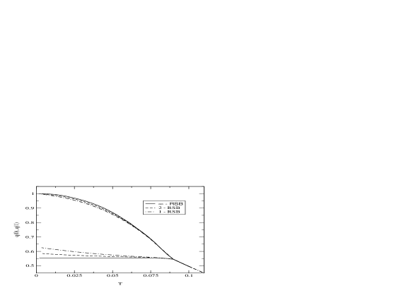
Figure 2: The order parameter at the slowest ($x=0$) and at the fastest ($x=1$) time scales as a function of reduced temperature. As the RSB scheme is improved the splitting between the two values increases.

For lower temperatures we used the Sommers’ gauge which takes an anomaly with constant derivative [25]. At difference with the SK, here we have two anomalies and hence two possible choices. However, the more natural one for numerical integration $\dot{\Delta}_{\lambda}(x)=-\Delta_{\lambda}(0)=const$ leads to a more involved determination of $\Delta_{\lambda}(0)$. Indeed we should first find $\dot{\Delta}_{q}(x)$ from eq. (26) and then $\Delta_{\lambda}(0)$ from (24). Therefore for low temperatures we adopted the Sommers’ gauge $\dot{\Delta}_{q}(x)=-\Delta_{q}(0)=const$ , where [see eq. (26)]:

$$\Delta_{q}(0)=-\beta\bigl{[}1-q(1)\bigr{]}+\int_{-\infty}^{\infty}dy\,P(0,y)\,m^{\prime}(0,y)$$ (40)

and $\dot{\Delta}_{\lambda}(x)=-\Delta_{q}(0)\,g_{2}(q(x))$. We note that since $\dot{\Delta}_{\lambda}$ does not vanish for $x\to 1$ this leads to numerical instabilities for large temperatures. Therefore from the point of view of numerical integration the two gauges are complementary.

The order parameters $q(x)$ and $\lambda(x)$ are different if we use the Parisi’s or the Sommers’ gauge, but the thermodynamics observables are, of course, invariant. This fact has been used to check the numerical integration by comparing the results from the two gauges in the temperature range where both are stable.

One of the main advantage of Sommers’ gauge is that we can solve the equations at exactly $T=0$. In Figure (3), for example, we report $q(x)$ for $T=0$ in the Sommers’ gauge. We recall that in the Parisi’s gauge $q(x)=q(1)$ for $x>0$ but $q(0)\not=q(1)$, as can also be inferred from Figure (1)

Figure 3: The order parameter $q(x)$ at zero temperature for the $3$-SAT, in the gauge $\dot{\Delta}_{q}=-\Delta_{q}(0)$.

For what concerns the thermodynamic quantities one sees that using (27) and (28) the entropy must be proportional to $T^{2}$ for $T\to 0$ and hence vanishes. Moreover it also follows that in the same limit $q(1)\simeq 1-aT^{2}$ [25, 30].

It can be easily checked that

$$\lim_{T\to 0}\left[f_{0}+\frac{\beta}{2}g\left(q(1)\right)\right]=\lim_{T\to 0}\left[\frac{\partial\beta f_{0}}{\partial\beta}+\beta g\left(q(1)\right)\right]=0$$ (41)

so that the energy density for $T=0$ can be written as

$$u=f_{v}=-\frac{1}{2}\int_{0}^{1}dx\ q(x)\ \dot{\Delta}_{\lambda}(x)-\int_{-\infty}^{\infty}dy\ P(0,y)\ \phi(0,y)\ .$$ (42)

The last term can be expressed as function of the local magnetization using the identity

$$\phi(0,y)=\phi(0,0)+\int_{0}^{y}dy_{1}\ m(0,y_{1})$$ (43)

where

$$\phi(0,0) = \int_{0}^{\infty}dy\left(1-m(0,y)\right)-\frac{1}{2}\int_{0}^{1}dx\ \dot{\Delta}_{\lambda}(x)$$ (44)

$$= \int_{0}^{\infty}dy\left(1-m(0,y)\right)+\frac{1}{2}\Delta_{q}(0)\int_{0}^{1}dxg_{2}\left(q(x)\right)\ .$$

Using the relations derived in the previous section, alternative expressions for $u$ can be obtained. For example by means of (34) evaluated for $T=0$ the energy density takes the form

$$f=u=-\int_{0}^{1}dx\ q(x)\ \dot{\Delta}_{\lambda}(x)-2\int_{0}^{\infty}dy\ y\ P(1,y)\ .$$ (45)

This can be simplified further using relation (37), which in the chosen gauge at $T=0$ becomes

$$\Delta_{q}(0)\int_{0}^{1}dx\ \left[q(x)\ g_{2}\left(q(x)\right)+g_{1}\left(q(x)\right)\right]=2\int_{0}^{\infty}dy\ P(1,y)\ y\ .$$ (46)

so that (45) takes the form:

$$u=\Delta_{q}(0)\int_{0}^{1}dx\ q(x)\ g_{2}\left(q(x)\right)-2\int_{0}^{\infty}dy\ y\ P(1,y)=-\Delta_{q}(0)\int_{0}^{1}dx\ g_{1}\left(q(x)\right)\ .$$ (47)

For the 3-SAT problem this reads:

$$u=-\frac{1}{128}\Delta_{q}(0)\int_{0}^{1}dx\ \left(1+q(x)\right)^{2}\ .$$ (48)

We conclude this section showing in Figure (4) the probability distribution $P(x,y)$ of frozen fields at $T=0$ for different time scales $\tau_{x}$. From the figure it is evident that the distribution of the field $y$ varies continuously from a Gaussian, for very short time-scales, to a double peak distribution, for the longest time-scales.

Figure 4: The local field probability distribution $P(x,y)$ for the $3$-SAT at T=0 in the Sommers’ gauge.

6 Thermodynamics of the highly constrained 3-SAT problem

In Figure (5) we show the entropy density as a function of temperature down to $T=0$. For each temperature, including $T=0$, the data are obtained using the gauge appropriate for that temperature. For comparison, the entropy computed within the Replica Symmetric, $1$-RSB and $2$-RSB solutions [14] are also plotted. As it can be seen from the log-lin plot, the $2$-RSB solution is a very good approximation but yet it is inexact when $T<0.016$. The entropy is zero for $T=0$ as confirming the conjecture of Ref. [6] for the behaviour in the UNSAT-phase. As expected, $s$ vanishes quadratically with the temperature.

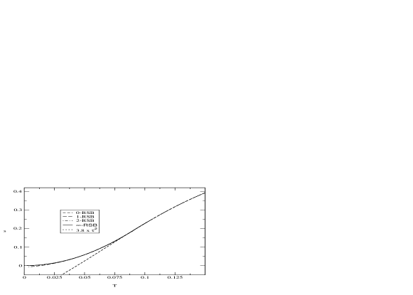
Figure 5: Entropy density of the $3$-SAT model for large number of clauses. The Replica Symmetric, $1$-RSB, $2$-RSB and $\infty$-RSB solutions are plotted. For the latter $s(0)=0$. On this scale the $2$-RSB and $\infty$-RSB are almost indistinguishable.

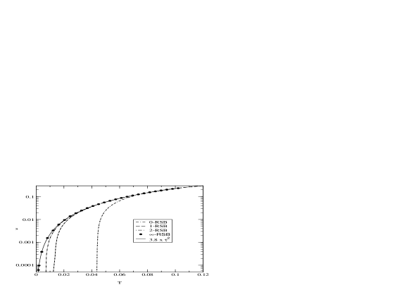
Figure 6: Same as Fig. (5) The improvement got in the low temperature region by breaking the replica symmetry is clearly seen. The data for $\infty$-RSB are reported as circle to distinguish them from the quadratic fit.

Finally in Figure (7) we show the energy density.

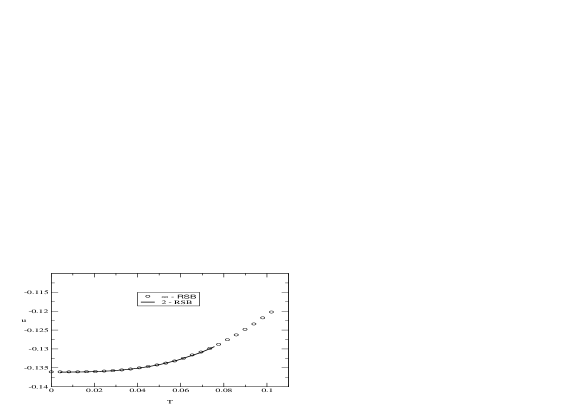
Figure 7: Energy density for the 3-SAT problem at high connectivity ($\alpha\gg\alpha_{c}$) in the 2-RSB and $\infty$-RSB solutions. The coincidence between the 2-RSB energy and the $\infty$-RSB energy is valid up to order $10^{-4}$.

The quantity plotted is actually $u(T)-\sqrt{\alpha}/48$, where $\alpha$ is very large. Equating the internal energy to zero we can determine an upper bound for the critical value $\alpha_{c}$ of the ratio of the number of clauses to the number of variables that marks the transition between the UNSAT-phase (in which we derived our asymptotic model) and the SAT-phase, where the energy is, by definition, always zero, at $T=0$. Using the $\infty$-RSB solution we get $\alpha_{c}^{\rm u.b.}=7.10969$. For the $2$-RSB solution it was already $\alpha_{c}^{\rm u.b.}=7.11400$ [14].

7 Conclusions

We performed the study of the Replica Symmetry Breaking solutions of the 3-SAT problem in the limit of many clauses, mapping it in a poorly diluted spin glass model with long-range random quenched interactions. The mapping to a statistical mechanics model was carried out introducing an artificial temperature and taking, in the end, the limit $T\to 0$, to recover the original model. We found that the structure of the solutions to the problem is of the $\infty$-RSB kind: in order to get a stable solution the replica symmetry has to be broken in a continuous way, similarly to the SK model [16] (in external magnetic field). The $\infty$-RSB structure holds down to the interesting limit of zero temperature.

No phase transition is expected in the UNSAT phase, other than the SAT-UNSAT transition occurring at $\alpha=\alpha_{c}\simeq 4.2$ Therefore we expect the same $\infty$-RSB structure of solutions of found for the over-constrained case to hold also in the critical region.

From the value of the energy at zero temperature we find the upper bound $\alpha_{c}<7.10969$. to the critical value of the number of clauses per variable. Even if this is of the same order of magnitude of $\alpha_{c}\simeq 4.2$ [7] yielded by direct numerical simulations, it is still too large. We recall that such a value has been obtained through a first order expansion in $1/\sqrt{\alpha}$. In order to get a better approximant other terms should be considered, possibly more then one since we are dealing with an asymptotic expansion and therefore nothing guarantees that the second order corrections are small and in the right direction.

Finally, as by product, in the present paper we worked out a precise procedure to get the $\infty$-RSB solution of a general class of models that, besides the over-constrained 3-SAT model, include SK, p-spin and, more generally, models with any combination of $p$ interacting terms. We presented the solution exploiting a variational method, introduced by Sommers and Dupont [25], which has the advantage of being easily implemented on a computer for any temperature including $T=0$. As a consequence the numerical code developed to solve the present model can be applied to the whole class of models without any relevant change, providing an efficient tool for the analysis of the structure of the solutions of a large number of spin models interacting via quenched random couplings.

References

References

- [1] M. R. Garey, D. S. Johnson, 1979, Computers and Intractability: A Guide to the Theory of NP-Completeness, Freeman, New York.
- [2] C. H. Papadimitriou, K. Steiglitz, 1982, Combinatorial Optimization: Algorithms and Complexity, Prentice Hall, Englewood Cliff, NJ.
- [3] S.A. Cook, 1971, “The complexity of theorem-proving procedures”, in Proc. 3rd Annu. ACM Symp. on Theory of Computing, Assoc. Comput. Machinery, New York, 151-158.
- [4] R.M. Karp, 1972, “Reducibility among combinatorial problems”, in R.E. Miller and J. W. Thatcher (eds.), Complexity of Computer Computations, Plenum Press, New York, 85-103.
- [5] R. Monasson, R. Zecchina, 1996, Phys. Rev. Lett. 76, 3881-3885.
- [6] R. Monasson, R. Zecchina, 1997, Phys. Rev. E 56, 1357-1370.
- [7] B. Selman, S. Kirkpatrick, 1996, Artif. Intell. 81, 273-295.
- [8] S. Kirkpatrick, C.D. Gelott Jr., M.P. Vecchi, 1983, Science 220, 339.
- [9] S. Kirkpatrick, B. Selman, 1994, Science 264, 1297-1301.
- [10] M. Mezard, G. Parisi, 2001, Eur. Phys. J. B 20 217-233.
- [11] S. Franz, M. Leone, F. Ricci-Tersenghi, R. Zecchina, Phys. Rev. Lett. 87, 127209 (2001).
- [12] R. Monasson, R. Zecchina, S. Kirkpatrick, B. Selman, L. Troyansky, 1999, Nature 400, 133.
- [13] G. Biroli, R. Monasson, M. Weigt, 2000, Eur. Phys. J. B 14, 551.
- [14] L. Leuzzi, G. Parisi, 2001, J. Stat. Phys. 103, 679.
- [15] We thank F. Zuliani and O. Martin for pointing this out.
- [16] D. Sherrington, S. Kirkpatrick, 1975, Phys. Rev. Lett. 26, 1782.
- [17] B. Derrida, 1980, Phys. Rev. Lett. 45, 79; D.J. Gross, M. Mezard, 1984, Nucl. Phys. B 240, 431; E. Gardner, 1985, Nucl. Phys. B 257, 747.
- [18] M. Mezard, G. Parisi, M.Virasoro, 1987, “Spin Glass Theory and Beyond”, World Scientific, Singapore.
- [19] K.H. Fischer and J.A. Hertz, “Spin Glasses”, 1991, Cambridge University Press, Cambridge, UK.
- [20] C. de Dominicis, M. Gabay, H. Orland, 1981, J. Phys. Lett. 42 L523.
- [21] C. de Dominicis, M. Gabay, B. Duplantier, 1982, J. Phys. A 15 L47-L49.
- [22] S.F. Edwards, P.W. Anderson, 1975, J. Phys. F 5 965.
- [23] H. Sompolinsky, 1981, Phys. Rev. Lett. 47 935.
- [24] G. Parisi, 1980, J. Phys. A 13, L115.
- [25] H. J. Sommers, W. Dupont, 1984, J. Phys. C 17 5785-5793.
- [26] K. Nemoto, 1987, J. Phys. C 20, 1325.
- [27] S. A. Orszag, 1971, Studies in applied mathematics Cambridge University, Cambridge, Vol. 4, p 293.
- [28] G. S. Patterson and S. A. Orszag, 1971, Phys. Fluids 14, 2538.
- [29] A. Crisanti and T. Rizzo, in preparation (2001).
- [30] D.J. Thouless, P.W. Anderson, R.G. Palmer, 1977, Phil. Mag. 35, 593.