Kinetics of formation of twinned structures under L1₀-type orderings in alloys

Abstract

The earlier-developed master equation approach and kinetic cluster methods are applied to study kinetics of L1₀-type orderings in alloys, including the formation of twinned structures characteristic of cubic-tetragonal-type phase transitions. A microscopical model of interatomic deformational interactions is suggested which generalizes a similar model of Khachaturyan for dilute alloys to the physically interesting case of concentrated alloys. The model is used to simulate A1$\to$L1₀ transformations after a quench of an alloy from the disordered A1 phase to the single-phase L1₀ state for a number of alloy models with different chemical interactions, temperatures, concentrations, and tetragonal distortions. We find a number of peculiar features in both transient microstructures and transformation kinetics, many of them agreeng well with experimental data. The simulations also demonstrate a phenomenon of an interaction-dependent alignment of antiphase boundaries in nearly-equilibrium twinned bands which seems to be observed in some experiments.

I Introduction

Studies of microstructural evolution under alloy phase transformations from the disordered FCC phase (A1 phase) to the CuAu I-type ordered tetragonal phase (L1₀ phase) attract interest from both fundamental and applied points of view. A characteristic feature of such transitions is the formation in the ordered phase of peculiar ‘polytwinned’ structures consisting of arrays of ordered bands separated by the antiphase boundaries (APBs) lying in the (110)-type planes, while the tetragonal axes of antiphase-ordered domains (APDs) in the adjacent bands have ‘twin-related’ (100) and (010)-type orientations [2, 3, 4, 5, 6, 7, 8]. Transformation A1$\to$L1₀ includes a number of intermediate stages, including the ‘tweed’ stage discussed below. These transformations are inherent, in particular, to many alloy systems with outstanding magnetic characteristics, such as Co–Pt, Fe–Pt, Fe–Pd and similar alloys, and studies of their microstructural features, for example, properties and evolution of APBs, are interesting for applications of these systems in various magnetic devices for which the structure and the distribution of APBs can be very important [3, 4, 5].

The physical reason for the formation of twinned structures was discussed by a number of authors [9, 10, 11, 12], and it is explained by the elimination of the volume-dependent part of elastic energy for such structures. However, theoretical treatments of the kinetics of A1$\to$L1₀ transformation seem to be rather scarce as yet. Khachaturyan and coworkers [13] discussed kinetics of tweed and twin formation using a 2D model in a square lattice with a number of simplifying approximations: a mean-field-type kinetic equation; a phenomenological description of interaction between elastic strains and local order parameters; an isotropic elasticity; an unrealistic interatomic interaction model (with the nearest-neighbour interaction being by an order of magnitude weaker than more distant interactions), etc. In spite of all these assumptions, some features of evolution found by Khachaturyan and coworkers [13] agree qualitatively with experimental observations [3, 4, 5]. It may illustrate a low sensitivity of these features to the real structure and interactions in an alloy. However, such an oversimplified approach is evidently insufficient to study the details of evolution and their dependence on the characteristics of an alloy, such as the type of interatomic interaction, concentration, temperature, etc, which seems to be most interesting for both applications and physical studies of the problem.

In this work we investigate kinetics of the A1$\to$L1₀ transition using the microscopical master equation approach and the kinetic cluster field method [14, 15]. Earlier this method was used to study A1$\to$L1₂-type transformations [16] as well as early stages of the A1$\to$L1₀ transition when the deformational interaction $H_{d}$ due to the tetragonal distortion of the L1₀ phase is still insignificant for the evolution [17]. Here we consider all stages of this transition, including the tweed and twin stages when the interaction $H_{d}$ becomes important. To this end we first derive a microscopical model for $H_{d}$ which generalizes the analogous model of Khachaturyan for dilute alloys [11] to the physically interesting case of concentrated alloys. Then we employ the kinetic cluster field method to simulate A1$\to$L1₀ transformation in the presence of deformational interaction $H_{d}$ for a number of alloy models with both short-range and extended-range chemical interactions at different temperatures, concentrations and tetragonal deformations. The simulations reveal a number of interesting microstructural features, many of them agreeing well with experimental observations [3, 4, 5]. We observe, in particular, a peculiar phenomenon of an interaction-dependent alignment of orientations of APBs within twin bands which was earlier discussed phenomenologically [12]. The simulations also show that the type of microstructural evolution strongly depends on the interaction type as well as on the concentration $c$ and temperature $T$. In particular, drastic, phase-transiton-like changes in morphology of APBs within twin bands can occur under variation of $c$ or $T$ in the short-range-interaction systems.

The paper is organized as follows. In section 2 we derive a microscopical expression for the deformational interaction $H_{d}$ in concentrated alloys. In section 3 we describe our methods of simulation of A1$\to$L1₀ transition which are similar to those used earlier [16, 17]. In section 4 we investigate the transformation kinetics for the alloy systems with an extended or intermediate interaction range, and in section 5, that for the short-range-interaction systems. Our main conclusions are summarized in section 6.

II Model for deformational interaction in concentrated alloys

We consider a binary substitutional alloy A_cB_1-c. Various distributions of atoms over lattice sites $i$ are described by the sets of occupation numbers $\{n_{i}\}$ where the operator $n_{i}=n_{{\rm A}i}$ is unity when the site $i$ is occupied by atom A and zero otherwise. The effective Hamiltonian $H_{\rm eff}$ describing the energy of these distributions has the form

$$H_{\rm eff}=\sum_{i>j}v_{ij}n_{i}n_{j}+\sum_{i>j>k}v_{ijk}n_{i}n_{j}n_{k}+\ldots$$ (1)

where $v_{i\ldots j}$ are effective interactions.

The interactions $v_{i\ldots j}$ include the ‘chemical’ contributions $v_{i\ldots j}^{c}$ which describe the energy changes under the substitution of some atoms A by atoms B in the rigid lattice, and the ‘deformational’ interactions $v_{i\ldots j}^{d}$ related to the difference in the lattice deformation under such a substitution. A microscopical model for $v^{d}$ in dilute alloys was suggested by Khachaturyan [11]. The deformational interaction in concentrated alloys can lead to some new effects that are absent in the dilute alloys, in particular, to the lattice symmetry changes under phase transformations, such as the tetragonal distortion under L1₀ ordering. Earlier these effects were treated only phenomenologically [13]. Below we describe a microscopical model for calculations of $v^{d}$ which generalizes the Khachaturyan’s approach [11] to the case of concentrated alloys.

Let us denote the position of site $k$ in the disordered ‘averaged’ crystal as ${\bf r}_{k}$. Because of the randomness of a real disordered or partially ordered alloy the actual atomic position (averaged over thermal vibrations) is not ${\bf r}_{k}$ but ${\bf r}_{k}+{\bf u}_{k}$ where ${\bf u}_{k}$ is the ‘static displacement’. Supposing this displacement to be small we can expand the ‘adiabatic’ (averaged over rapid phonon motion) alloy energy $H=H\{n_{i},{\bf u}_{k}\}$ to second order in ${\bf u}_{k}$:

$$H=H_{c}\{n_{i}\}-\sum_{k}u_{\alpha k}F^{\alpha k}+{1\over 2}\sum_{k,l}u_{\alpha k}u_{\beta l}A_{\alpha k,\beta l}$$ (2)

where $\alpha$ and $\beta$ are Cartesian indices and the summation over repeated Greek indices is implied here and below. The term $H_{c}\{n_{i}\}$ in (2) describes interactions in the undistorted average crystal lattice, i. e. chemical interactions $v_{i\ldots j}^{c}$ mentioned above; $F^{\alpha k}$ can be called the generalized Kanzaki force; and $A_{\alpha k,\beta l}$ is the force constant matrix. Both quantities $F^{\alpha k}$ and $A_{\alpha k,\beta l}$ are certain functions of occupation numbers $n_{i}$, and their evaluation needs some further approximations.

Below we consider ordering phase transitions at the fixed mean concentration $c$. Changes of elastic constants and phonon spectra under such transitions are usually small[18]. Therefore, the force constant matrix $A_{\alpha k,\beta l}$ can be reasonably well approximated with the simple ‘average crystal’ approximation: $A_{\alpha k,\beta l}\{n_{i}\}\rightarrow A_{\alpha k,\beta l}\{c\}\equiv\overline{A}_{\alpha k,\beta l}$. To approximate the Kanzaki force $F^{\alpha k}$ we first formally write it as a series in the occupation numbers $n_{i}$:

$$F^{\alpha k}\{n_{i}\}=F^{\alpha k}_{0}+\sum_{i}F^{\alpha k,i}_{1}n_{i}+\sum_{i>j}F^{\alpha k,ij}_{2}n_{i}n_{j}+\ldots$$ (3)

Equilibrium values of displacements ${\bf u}_{k}={\bf u}_{k}^{e}\{n_{i}\}$ at the given distribution $\{n_{i}\}$ are determined by the minimization of energy (2) over ${\bf u}_{k}$, and the constant $F^{\alpha k}_{0}$ in (3) affects only the reference point ${\bf u}_{k}^{e}\{0\}$ in the function ${\bf u}_{k}^{e}\{n_{i}\}$. This constant can be determined, for example, from the condition of vanishing of mean static displacements in the averaged crystal at some $c=c_{0}$, which implies the relation: $\langle F^{\alpha k}\{n_{i}\}\rangle_{c=c_{0}}=0$ where the symbol $\langle\ldots\rangle$ means the statistical averaging over an alloy. The constants $F^{\alpha k}_{0}$ are insignificant for what follows, and below they are omitted to simplify formulas.

In writing an explicit expression for the contribution $H_{K}$ (to be called for brevity the ‘Kanzaki term’) of the occupation-dependent Kanzaki forces in energy (2) one should consider that due to the translation invariance it can include only differences of displacements $({\bf u}_{k}-{\bf u}_{i})$, $({\bf u}_{k}-{\bf u}_{j})$, etc. Therefore, this term should have the form

$$H_{K}=\sum_{k,i}({\bf u}_{i}-{\bf u}_{k}){\bf f}^{k,i}_{1}n_{i}+\sum_{k,ij}({\bf u}_{i}-{\bf u}_{k}){\bf f}^{k,ij}_{2}n_{i}n_{j}+\ldots$$ (4)

where ${\bf f}^{k,i_{1}\ldots i_{m}}_{m}\equiv{\bf f}^{k}_{m}$ are some parameters describing interaction of lattice deformations with site occupations.

Representation (4) for $H_{K}$ as a sum of contributions of $m$-site ‘clusters’ proportional to products $n_{i_{1}}\ldots n_{i_{m}}$ is analogous to similar cluster expansions for the ‘chemical’ Hamiltonian $H_{c}\{n_{i}\}$ in (2). These expansions have been widely discussed, in particular, in connection with first-principle calculations of chemical interactions $v^{c}_{i_{1}\ldots i_{m}}\equiv v^{c,m}$, see e. g. [19]. The calculations have shown that the values of $m$-site interactions $v^{c,m}$ in most alloys rapidly decrease with an increase of $m$, and the pairwise interaction $v^{c,2}$ is usually dominant. It is natural to expect that a similar rapid convergence is also typical for the expansion (4). Therefore, below we omit many-site interactions ${\bf f}^{k}_{m}$ with $m>2$ in Eq. (4). At the same time, in estimates of parameters ${\bf f}^{k}_{m}$ for real alloys below we combine some model assumptions about ${\bf f}^{k}_{m}$ with using of available experimental data about the variations of lattice deformations with concentration and orderings, and such estimates may also implicitly include the contributions of many-site interactions ${\bf f}^{k}_{m}$.

For what follows it is convenient to proceed from functions ${\bf u}_{k}={\bf u}({\bf r}_{k})$, $n_{i}=n({\bf r}_{i})$, ${\bf f}_{1}^{k,i}={\bf f}_{1}({\bf r}_{k}-{\bf r}_{i})$, ${\bf f}_{2}^{k,ij}={\bf f}_{2}({\bf r}_{k}-{\bf r}_{i},{\bf r}_{j}-{\bf r}_{i})$ and $\overline{A}_{\alpha k,\beta l}=\overline{A}_{\alpha\beta}({\bf r}_{k}-{\bf r}_{l})$ in Eqs. (2) and (4) to their Fourier components in the average crystal lattice. Then the energy (2) takes the form:

$$H=H_{c}\{n_{i}\}+{\frac{1}{N}}\sum_{\bf k}{\bf u}_{-{\bf k}}\left(n_{\bf k}{\bf f}_{1{\bf k}}+\sum_{\bf R}\sigma_{\bf k}^{\bf R}{\bf f}_{2{\bf k}}^{\bf R}\right)+{\frac{1}{2N}}\sum_{\bf k}u_{-{\bf k}}^{\alpha}\overline{A}_{\bf k}^{\alpha\beta}u_{{\bf k}}^{\beta}.$$ (5)

Here $N$ is the total number of crystal cells, the summation over $\bf k$ goes within the Brillouin zone of the averaged crystal, and we use the following notation:

$${\bf u}_{\bf k}=\sum_{\bf r}{\bf u}({\bf r})e^{-i\bf{kr}};\qquad\hskip 17.07164ptn_{\bf k}=\sum_{\bf r}n({\bf r})e^{-i\bf{kr}};\qquad\sigma_{\bf k}^{\bf R}=\sum_{\bf r}n({\bf r})n({\bf r}+{\bf R})e^{-i\bf{kr}};$$ (6)

$${\bf f}_{1{\bf k}}=\sum_{\bf r}{\bf f}_{1}({\bf r})(1-e^{-i\bf{kr}});\quad{\bf f}_{2{\bf k}}^{\bf R}=\sum_{\bf r}{\bf f}_{2}({\bf r,\bf R})(1-e^{-i\bf{kr}});\quad\overline{A}_{\bf k}^{\alpha\beta}=\sum_{\bf r}\overline{A}_{\alpha\beta}({\bf r})e^{-i\bf{kr}}.$$ (7)

If one adopts a commonly used model of ‘central’ Kanzaki forces in which forces ${\bf f}_{1}^{k,i}$ and ${\bf f}_{2}^{k,ij}$ in (4) are supposed to be proportional to the vector ${\bf r}_{ki}=({\bf r}_{k}-{\bf r}_{i})$, the vector functions ${\bf f}_{1{\bf k}}$ and ${\bf f}_{2{\bf k}}$ in (7) can be expressed via two scalar functions, $\varphi_{1}$ and $\varphi_{2}$:

$${\bf f}_{1{\bf k}}=\sum_{\bf r}{\bf r}\,\varphi_{1}(r)\,(1-e^{-i\bf{kr}}),\quad{\bf f}_{2{\bf k}}^{\bf R}=\sum_{\bf r}{\bf r}\,\varphi_{2}({\bf r,\bf R})\,(1-e^{-i\bf{kr}}).$$ (8)

The functions $\varphi_{1}$ and $\varphi_{2}$ in (8) determine the dependence of equilibrium lattice parameters on concentration or ordering. To show it we first note that the homogeneous deformation $\overline{u}_{\alpha\beta}$ is described by Fourier-components ${\bf u}_{\bf k}$ with small ${\bf k}\to 0$, while functions ${\bf f}_{1{\bf k}}$ and ${\bf f}_{2{\bf k}}$ in Eqs. (5) and (7) at small ${\bf k}$ are linear in ${\bf k}$. Thus the contribution of homogeneous deformations to the Kanzaki term in (5) is proportional to Fourier-components $u^{\alpha\beta}_{\bf k}$ of the elastic strain $u_{\alpha\beta}=(\partial u_{\alpha}/\partial x_{\beta}+\partial u_{\beta}/\partial x_{\alpha})/2$ at ${\bf k}\to 0$ and, according to first equation (7), these components are related to $\overline{u}_{\alpha\beta}$ as

$$u^{\alpha\beta}_{\bf k}|_{{\bf k}\to 0}=i(k_{\beta}u_{\bf k}^{\alpha}+k_{\alpha}u_{\bf k}^{\beta})|_{{\bf k}\to 0}=N\overline{u}_{\alpha\beta}.$$ (9)

At small $\bf k$ the force constant matrix $\overline{A}_{\bf k}^{\alpha\beta}$ in (5) is bilinear in $\bf k$, and the last term of (5) corresponds to the standard expression for the elastic energy bilinear in $\overline{u}_{\alpha\beta}$ and linear in the elastic constants $c_{\alpha\beta\gamma\delta}$, see e.g. [11]. Therefore, the total contribution of terms with the homogeneous elastic strain $\overline{u}_{\alpha\beta}$ to energy (5) (to be called ‘the elastic strain energy’ $E_{el}$) can be written as

$$E_{el}=-\overline{u}_{\alpha\beta}\left(A_{1}^{\alpha\beta}n_{0}+\sum_{\bf R}A_{2{\bf R}}^{\alpha\beta}\sigma_{0}^{\bf R}\right)+{\frac{1}{2}}N\Omega\,c_{\alpha\beta\gamma\delta}\overline{u}_{\alpha\beta}\overline{u}_{\gamma\delta}.$$ (10)

Here $\Omega$ is the volume per atom in the average crystal; quantities $A_{1}^{\alpha\beta}$ and $A_{2{\bf R}}^{\alpha\beta}$ are expressed via functions $\varphi_{1}$ and $\varphi_{2}$ in (8) as:

$$A_{1}^{\alpha\beta}=\sum_{\bf r}x_{\alpha}x_{\beta}\varphi_{1}({\bf r}),\qquad A_{2{\bf R}}^{\alpha\beta}=\sum_{\bf r}x_{\alpha}x_{\beta}\varphi_{2}({\bf r},{\bf R}),$$ (11)

where $x_{\alpha}$ is the Cartesian component of vector ${\bf r}=(x_{1},x_{2},x_{3})$; and $n_{0}$ or $\sigma_{0}^{\bf R}$ is the Fourier component, $n_{\bf k}$ or $\sigma_{\bf k}^{\bf R}$, at ${\bf k}=0$. According to Eq. (7), the operator $n_{0}$ or $\sigma_{0}^{\bf R}$ is the sum of a macroscopically large number $N$ of similar terms. Thus within the statistical accuracy each of these operators can be substituted by its average value:

$$n_{0}=N\langle n({\bf r})\rangle=Nc;\qquad\sigma_{0}^{\bf R}=N\langle n({\bf r})\,n({\bf r}+{\bf R})\rangle.$$ (12)

The last average in (12) can be expressed via mean occupations of sites and their correlators. In an ordered alloy there exist several non-equivalent sublattices $s$ with the lattice vectors ${\bf r}_{s}$ and mean occupations $c_{s}=\langle n({\bf r}_{s})\rangle$, and so the last average in (12) includes averaging over all sublattices $s$:

$$\langle n({\bf r})\,n({\bf r}+{\bf R})\rangle=\sum_{s}\nu_{s}\left(c_{s}\,c_{s{\bf R}}+K_{s{\bf R}}\right).$$ (13)

Here $c_{s{\bf R}}$ is the mean occupation $\langle n({\bf r})\rangle$ for ${\bf r}={\bf r}_{s}+{\bf R}$; $\nu_{s}=N_{s}/N$ is the relative number of sites in the sublattice $s$; and $K_{s{\bf R}}$ is the correlator of occupations of sites located at ${\bf r}={\bf r}_{s}$ and at ${\bf r}={\bf r}_{s}+{\bf R}$:

$$K_{s{\bf R}}=\langle\left[n({\bf r}_{s})-c_{s}\right]\left[n({\bf r}_{s}+{\bf R})-c_{s{\bf R}}\right]\rangle.$$ (14)

In a disordered alloy all sites are equivalent, thus $c_{s}=c_{s{\bf R}}=c$;   $\nu_{s}=1$; and both index $s$ and the summation over $s$ in (13) are omitted.

Using Eqs. (12) and (13) one can rewrite the elastic strain energy (10) as

$$E_{el}=-N\overline{u}_{\alpha\beta}\left[A_{1}^{\alpha\beta}\,c+\sum_{\bf R}\sum_{s}\nu_{s}\left(c_{s}\,c_{s{\bf R}}+K_{s{\bf R}}\right)A_{2{\bf R}}^{\alpha\beta}\right]+{\frac{1}{2}}N\Omega\,c_{\alpha\beta\gamma\delta}\overline{u}_{\alpha\beta}\overline{u}_{\gamma\delta}.$$ (15)

The correlator $K_{s{\bf R}}$ in Eq. (15) can be calculated using that or another method of statistical theory. However, for most alloy systems of practical interest, in particular, at $c$ and $T$ values not close to the thermodynamic instabilty points $T_{s}$, the correlators $K_{s{\bf R}}$ are small and can be neglected. Then equation (15) is simplified:

$$E_{el}=-\overline{u}_{\alpha\beta}\left[NA_{1}^{\alpha\beta}\,c+\sum_{{\bf r},{\bf R}}c({\bf r})c({\bf r}+{\bf R})A_{2{\bf R}}^{\alpha\beta}\right]+{\frac{1}{2}}N\Omega\,c_{\alpha\beta\gamma\delta}\overline{u}_{\alpha\beta}\overline{u}_{\gamma\delta}.$$ (16)

Equilibrium values of $\overline{u}_{\alpha\beta}$ in the absence of applied stress are determined by the minimization of energy $E_{el}$ with respect to $\overline{u}_{\alpha\beta}$ which gives:

$$\Omega\,c_{\alpha\beta\gamma\delta}\overline{u}_{\gamma\delta}=A_{1}^{\alpha\beta}\,c+{\frac{1}{N}}\sum_{{\bf r},{\bf R}}c({\bf r})c({\bf r}+{\bf R})A_{2{\bf R}}^{\alpha\beta}.$$ (17)

Eq. (17) enables one to express the equilibrium strain $\overline{u}_{\alpha\beta}$ via the concentration, order parameters, and the interaction parameters $A_{1}^{\alpha\beta}$ and $A_{2{\bf R}}^{\alpha\beta}$, and it can also be used to estimate these interaction parameters from experimental data on $\overline{u}_{\alpha\beta}(c,T)$.

Let us consider Eqs. (16) and (17) in particular cases. For a disordered phase with $c({\bf r})=c$,   Eq. (17) takes the form

$$\Omega\,c_{\alpha\beta\gamma\delta}\overline{u}_{\gamma\delta}=A_{1}^{\alpha\beta}\,c+A_{2}^{\alpha\beta}\,c^{2}$$ (18)

where $A_{2}^{\alpha\beta}=\sum_{\bf R}A_{2{\bf R}}^{\alpha\beta}$. If the disordered phase has a cubic symmetry (as for the FCC or BCC alloys), quantities $A_{1}^{\alpha\beta}$ and $A_{2}^{\alpha\beta}$ are proportional to the Kronecker symbol $\delta_{\alpha\beta}$, and Eq. (18) determines the concentrational dilatation $u(c)=\overline{u}_{\alpha\alpha}(c)-u_{\alpha\alpha}(0)$:

$$u(c)=(A_{1}c+A_{2}c^{2})/\Omega B.$$ (19)

Here $B=(c_{11}+2c_{12})/3$ is the bulk modulus; $c_{ij}$ are the elastic constants in Voigt’s notation; and coefficients $A_{1}$ and $A_{2}$ are expressed via functions $\varphi_{1}$ and $\varphi_{2}$ in (8), (11):

$$A_{1}=\sum_{\bf r}\varphi_{1}({\bf r})r^{2}/3;\qquad A_{2}=\sum_{{\bf r},{\bf R}}\varphi_{2}({\bf r},{\bf R})r^{2}/3.$$ (20)

The linear in $c$ term in (19) corresponds to the Vegard law while the term with $A_{2}$ describes the non-linear deviations from this law. Such deviations were observed for many alloys, and these data can be used to estimate $A_{2}$ values, but in these estimates one should also take into consideration a possible concentration dependence of the bulk modulus $B$.

For the ordered phase, the mean occupation $c({\bf r})$ can be written as a superposition of concentration waves corresponding to certain superstructure vectors ${\bf k}_{p}$ [11]:

$$c({\bf r})=c+{1\over 2}\sum_{p}\left[\eta_{p}\exp(i{\bf k}_{p}{\bf r})+\eta_{p}^{*}\exp(-i{\bf k}_{p}{\bf r})\right],$$ (21)

and amplitudes $\eta_{p}$ can be considered as order parameters. After the substitution of expressions (21) for $c({\bf r})$ and $c({\bf r}+{\bf R})$ in Eq. (16) the linear in $\eta_{p}$ terms vanish due to the crystal symmetry, and the first term of (16) becomes the sum of the ordering-independent term and the term bilinear in order parameters:

$$E_{el}=-N\overline{u}_{\alpha\beta}\left(A_{1}^{\alpha\beta}\,c+A_{2}^{\alpha\beta}\,c^{2}+\sum_{p}q_{\alpha\beta pp}|\eta_{p}|^{2}\right)+{\frac{1}{2}}N\Omega\,c_{\alpha\beta\gamma\delta}\overline{u}_{\alpha\beta}\overline{u}_{\gamma\delta}.$$ (22)

Here quantities $q_{\alpha\beta pp}$ have a different form in the cases ($a$) when the superstructure vector ${\bf k}_{p}$ is half of some reciprocal lattice vector ${\bf g}$ and thus both the order parameter $\eta_{p}$ and all factors $\exp(i{\bf k}_{p}{\bf r})$ in (21) are real, and ($b$) when ${\bf k}_{p}\neq{\bf g}/2$:

$$(a)\qquad{\bf k}_{p}={\bf g}/2:\hskip 28.45274ptq_{\alpha\beta pp}=\sum_{{\bf r},{\bf R}}x_{\alpha}x_{\beta}\varphi_{2}({\bf r},{\bf R})\exp\,(i{\bf k}_{p}{\bf r});$$ (23)

$$(b)\qquad{\bf k}_{p}\neq{\bf g}/2:\hskip 28.45274ptq_{\alpha\beta pp}={1\over 2}\sum_{{\bf r},{\bf R}}x_{\alpha}x_{\beta}\varphi_{2}({\bf r},{\bf R})\cos\,({\bf k}_{p}{\bf r}).$$ (24)

The coefficients $q_{\alpha\beta pp}$ in (22) (to be called the ‘striction’ coefficients, in an analogy with the terminology used in the ferroelectricity or magnetism theory) are commonly used in phenomenological theories of lattice distortions under orderings [9, 10, 11, 12, 13]. Eqs. (23), (24) and (11) provide the microscopic expression for these coefficients via the function $\varphi_{2}$ describing non-pairwise Kanzaki forces in Eqs. (5)–(8).

Let us apply Eqs. (21)–(23) to the case of L1₀ or L1₂ ordering in FCC alloys which are described by three real order parameters $\eta_{\alpha}$ [11, 16]. Eqs. (21) here take the form

$$c({\bf r})=c+\eta_{1}\exp(i{\bf k}_{1}{\bf r})+\eta_{2}\exp(i{\bf k}_{2}{\bf r})+\eta_{3}\exp(i{\bf k}_{3}{\bf r}),$$ (25)

where ${\bf k}_{\alpha}={\bf g}_{\alpha}/2$ is the superstructure vector corresponding to $\eta_{\alpha}$:

$${\bf k_{1}}=[100]2\pi/a,\qquad{\bf k_{2}}=[010]2\pi/a,\qquad{\bf k_{3}}=[001]2\pi/a.$$ (26)

In the cubic L1₂ structure one has: $|\eta_{1}|=|\eta_{2}|=|\eta_{3}|$, $\eta_{1}\eta_{2}\eta_{3}>0$, and four types of ordered domains are possible. In the L1₀-ordered structure with the tetragonal axis $\alpha$ a single parameter $\eta_{\alpha}$ is present which is either positive or negative, and so six types of ordered domains are possible.

The striction coefficients for L1₀ or L1₂ ordering are determined by Eq. (23). Due to the cubic symmetry of the ‘average’ FCC crystal, there are only two different striction coefficients, $q_{1111}$ and $q_{1122}$ (and those obtained from them by the cubic symmetry operations), which for brevity will be denoted as $q_{11}$ and $q_{12}$, respectively:

$$q_{11}=\sum_{{\bf r},{\bf R}}x_{1}^{2}\varphi_{2}({\bf r},{\bf R})\exp(i{\bf k}_{1}{\bf R});\quad q_{12}=\sum_{{\bf r},{\bf R}}x_{1}^{2}\varphi_{2}({\bf r},{\bf R})\exp(i{\bf k}_{2}{\bf R}).$$ (27)

Variation of elastic constants $c_{\alpha\beta\gamma\delta}$ with ordering is usually small[18], and for simplicity it will be neglected. Then minimizing energy (22) with respect to $\overline{u}_{\alpha\beta}$ we obtain the expressions for lattice deformations induced by ordering (25):

$$\overline{u}=q_{+}(\eta_{1}^{2}+\eta_{2}^{2}+\eta_{3}^{2})/\Omega c_{+},\quad\overline{\varepsilon}=q_{-}[\eta_{1}^{2}-(\eta_{2}^{2}+\eta_{3}^{2})/2]/\Omega c_{-},\quad\zeta=q_{-}(\eta_{2}^{2}-\eta_{3}^{2})/\Omega c_{-}.$$ (28)

Here $\overline{u}=\overline{u}_{11}+\overline{u}_{22}+\overline{u}_{33}$ describes the volume change; $\overline{\varepsilon}=\overline{u}_{11}-(\overline{u}_{22}+\overline{u}_{33})/2$ is the tetragonal distortion; $\zeta=\overline{u}_{22}-\overline{u}_{33}$ is the shear deformation; and $q_{\pm}$ or $c_{\pm}$ are linear combinations of striction or elastic constants:

$$q_{-}=q_{11}-q_{12};\quad c_{-}=c_{11}-c_{12};\quad q_{+}=q_{11}+2q_{12};\quad c_{+}=c_{11}+2c_{12}.$$ (29)

For the L1₂ ordering, values $|\eta_{1}|=|\eta_{2}|=|\eta_{3}|=\eta$ are the same, so just the volume striction $\overline{u}=3q_{+}\eta^{2}/\Omega c_{+}$ is present, while in the L1₀-ordered domain with $\eta_{2}=\eta_{3}=0$ one has both the volume and the tetragonal striction:

$$\overline{u}=q_{+}\eta_{1}^{2}/\Omega c_{+},\qquad\overline{\varepsilon}=q_{-}\eta_{1}^{2}/\Omega c_{-}.$$ (30)

Therefore, using experimental data about the lattice distortions and order parameters under L1₂ and L1₀ orderings one can estimate the striction coefficients $q_{11}$ and $q_{12}$ and thus the non-pairwise Kanzaki interaction $\varphi_{2}$ in Eqs. (27).

Below we suppose for simplicity the interaction $\varphi_{2}({\bf r},{\bf R})$ to be short-ranged, i. e. significant only when each of three relative distances $r$, $R$ and $|{\bf r}-{\bf R}|$ does not exceed the nearest-neighbour distance $\rho=a/\sqrt{2}$. Then this function can be written as

$$\varphi_{2}({\bf r},{\bf R})=\delta_{r,\rho}\delta_{R,\rho}\left(\varphi_{a}\,\delta_{|{\bf r}-{\bf R}|,0}+\varphi_{b}\,\delta_{|{\bf r}-{\bf R}|,\rho}\right)$$ (31)

where $\delta_{r,\rho}$ is the Kronecker symbol equal to unity when $r=\rho$ and zero otherwise while $\varphi_{a}$ and $\varphi_{b}$ are the interaction parameters. The assumption (31) is analogous to that used by Khachaturyan [11] for the pairwise Kanzaki interaction $\varphi_{1}({\bf r})$ in (8):

$$\varphi_{1}({\bf r})=\varphi_{1}\delta_{r,\rho}$$ (32)

where the constant $\varphi_{1}$ is estimated from experimental data on concentrational dilatation. First-principle estimates of lattice distortions in dilute alloys [20] seem to imply that the assumption (32) yields the correct order of magnitude of $\varphi_{1}({\bf r})$. Therefore, the analogous assumption (31) for $\varphi_{2}({\bf r},{\bf R})$ can be reasonable, too.

Substituting Eq. (31) into (27) we obtain the explicit expression for coefficients $q_{ik}$ via parameters $\varphi_{a}$ and $\varphi_{b}$ in (31):

$$q_{11}=-2a^{2}\varphi_{a};\qquad q_{12}=-4a^{2}\varphi_{b}.$$ (33)

The coefficient ${\bf f}_{1{\bf k}}$ in Eqs. (5) and (7) for model (32) has the form [11]:

$${\bf f}_{1{\bf k}}=4\varphi_{1}i\sum_{\alpha=1}^{3}{\bf a}_{\alpha}\sin\,({\bf ka}_{\alpha})\sum_{\beta\neq\alpha}\cos\,({\bf ka}_{\beta})$$ (34)

where ${\bf a}_{\alpha}$ is ${\bf e}_{\alpha}a/2$ and ${\bf e}_{\alpha}$ is the unit vector along the main crystal axis $\alpha$. The function ${\bf f}_{2{\bf k}}^{\bf R}$ in (5), (7) for model (31) is the sum of two terms:

$${\bf f}_{2{\bf k}}^{\bf R}={\bf f}_{a{\bf k}}^{\bf R}+{\bf f}_{b{\bf k}}^{\bf R}.$$ (35)

Here, ${\bf f}_{a{\bf k}}^{\bf R}$ is $\varphi_{a}\delta_{R,\rho}{\bf R}\left(1-e^{-i{\bf kR}}\right)$, while the function ${\bf f}_{b{\bf k}}^{\bf R}$ for ${\bf R}$ equal to ${\bf R}_{\alpha}+{\bf R}_{\beta}$ (where ${\bf R}_{\alpha}$ is ${\bf a}_{\alpha}$ or $(-{\bf a}_{\alpha})$, ${\bf R}_{\beta}$ is ${\bf a}_{\beta}$ or $(-{\bf a}_{\beta})$, and $\beta\neq\alpha$) can be written as

$${\bf f}_{b{\bf k}}^{\bf R}=2\varphi_{b}\left[{\bf R}+\left(i{\bf a^{\prime}}\sin{\bf ka^{\prime}}-{\bf R}_{\alpha}\cos\,{\bf ka^{\prime}}\right)e^{-i{\bf kR}_{\alpha}}+\left(i{\bf a^{\prime}}\sin{\bf ka^{\prime}}-{\bf R}_{\beta}\cos\,{\bf ka^{\prime}}\right)e^{-i{\bf kR}_{\beta}}\right]$$ (36)

where ${\bf a^{\prime}}$ is $[{\bf e}_{\alpha}{\bf e}_{\beta}]a/2$.

Relations (8), (31)–(36) together with (19) and (33) provide a simplified model for the Kanzaki term $H_{K}$ in Eqs. (4) and (5). This model will be used below in simulations of A1$\to$L1₀ transitions. To get an idea about the actual scale of parameters of this model, let us estimate quantities $q_{ik}$, $\varphi_{a}$ and $\varphi_{b}$ in Eqs. (31) and (33) for the alloys Co–Pt for which detailed data about the lattice distortion under L1₂ and L1₀ orderings are available [21, 22]. The volume change $\overline{u}$ under both the L1₂ ordering in CoPt₃ and L1₀ ordering in CoPt appears to be very small [21, 22, 2]: $\overline{u}\lesssim 10^{-3}$. According to Eqs. (28) and (30) it implies the relation: $q_{12}\simeq q_{11}/2$. The value $q_{-}=(q_{11}-q_{12})$ for CoPt can be estimated from second equation (30) using data of Ref. [22] for $\eta_{1}$ and $\overline{\varepsilon}$ at $T=0.84\,T_{c}$:  $\eta_{1}\simeq 0.4$;   $\varepsilon\simeq-0.04$ (with the thermal expansion effect subtracted); and for the atomic volume: $\Omega=\Omega(T_{c}+0)\simeq 13.8{\rm\AA}^{3}$. Using also for the elastic constant $c_{-}=(c_{11}-c_{12})$ its value for the FCC platinum, $c_{-}\simeq 0.97$ Mbar [23], we obtain: $q_{-}\simeq 2.6\cdot 10^{4}$ K. Combining it with the above-mentioned relation $q_{12}\simeq q_{11}/2$ and using Eq. (28) we find: $\varphi_{a}\simeq 2\cdot 10^{4}$ K$/a^{2}$, and $\varphi_{b}\simeq 5\cdot 10^{3}$ K$/a^{2}$. Let us also note that the ordering-induced elastic energy per atom $\varepsilon_{el}^{ord}$ in the CoPt alloy is small: $\varepsilon_{el}^{ord}\simeq\Omega c_{-}\overline{\varepsilon}^{2}/6\simeq$ 30 K, which is much less than the L1₀ ordering temperature $T_{c}\simeq 1100$ K.

The equilibrium values of displacements ${\bf u}_{\bf k}^{e}={\bf u}_{\bf k}^{e}(n_{i})$ are found by the minimization of energy (5) over ${\bf u_{k}}$. Substituting these ${\bf u}_{\bf k}^{e}$ into Eq. (5) we obtain the effective Hamiltonian $H=H_{c}+H_{d}$ where the deformational interaction $H_{d}$ can be written as

$$H_{d}=-{\frac{1}{2N}}\sum_{\bf k}\left(n_{-\bf k}{\bf f}_{1{\bf k}}^{*}+\sum_{\bf R}\sigma_{-\bf k}^{\bf R}{\bf f}_{2{\bf k}}^{{\bf R}*}\right){\bf G_{k}}\left(n_{\bf k}{\bf f}_{1{\bf k}}+\sum_{\bf R}\sigma_{\bf k}^{\bf R}{\bf f}_{2{\bf k}}^{\bf R}\right)=H_{d2}+H_{d3}+H_{d4}.$$ (37)

Here the matrix ${\bf G_{k}}=G_{\bf k}^{\alpha\beta}$ is inverse to the force constant matrix $\overline{A}_{\bf k}^{\alpha\beta}$, and the matrix product $\bf aBc$ means the sum $a_{\alpha}B_{\alpha\beta}b_{\beta}$. The term $H_{d2}$, $H_{d3}$ and $H_{d4}$ in (37) describes the pairwise, three-particle and four-particle deformational interaction, respectively:

$$H_{d2}={\frac{1}{2}}\sum_{\bf r,r^{\prime}}n({\bf r})\Phi_{2}({\bf r}-{\bf r^{\prime}})n({\bf r^{\prime}}),\qquad H_{d3}={\frac{1}{2}}\sum_{\bf r,r^{\prime}}\sum_{\bf R}n({\bf r})\Phi_{3}^{\bf R}({\bf r}-{\bf r^{\prime}})n({\bf r^{\prime}})n({\bf r^{\prime}}+{\bf R}),$$ (38)

$$H_{d4}={\frac{1}{2}}\sum_{\bf r,r^{\prime}}\sum_{\bf,R,R^{\prime}}n({\bf r})n({\bf r}+{\bf R})\Phi_{4}^{\bf R,R^{\prime}}({\bf r}-{\bf r^{\prime}})n({\bf r^{\prime}})n({\bf r^{\prime}}+{\bf R^{\prime}}),$$ (39)

where the potential $\Phi_{2}$, $\Phi_{3}^{\bf R}$ or $\Phi_{4}^{\bf R,R^{\prime}}$ is given by the expression:

$$\left\{\Phi_{2}({\bf r});\Phi_{3}^{\bf R}({\bf r});\Phi_{4}^{\bf R,R^{\prime}}({\bf r})\right\}=-{\frac{1}{N}}\sum_{\bf k}e^{i{\bf kr}}\left\{{\bf f}_{1{\bf k}}^{*}{\bf G_{k}}{\bf f}_{1{\bf k}};\ {\bf f}_{1{\bf k}}^{*}{\bf G_{k}}{\bf f}_{2{\bf k}}^{{\bf R}}+{\bf f}_{2{\bf k}}^{{\bf R}*}{\bf G_{k}}{\bf f}_{1{\bf k}};\ {\bf f}_{2{\bf k}}^{{\bf R}*}{\bf G_{k}}{\bf f}_{2{\bf k}}^{{\bf R^{\prime}}}\right\}.$$ (40)

As the matrix ${\bf G_{k}}$ in (40) at small $k$ includes the well-known ‘elastic singularity’ [11]: ${\bf G_{k}}\sim 1/k^{2}$, each of terms $H_{d2}$, $H_{d3}$ and $H_{d4}$ in (37) includes the long-ranged elastic interaction. The formation of twinned structures discussed below is determined by the four-particle interaction $H_{d4}$. The rest deformational interactions, $H_{d2}$ and $H_{d3}$, for the single-phase L1₀ ordering under consideration lead just to some quantitative renormalizations of chemical interaction $H_{c}$ in (5) which are usually small and insignificant. Therefore, below we retain in the deformational interaction (37) only the last term $H_{d4}$. Let us also note that each term in the sum (39) for $H_{d4}$ at fixed $\bf r$ and $\bf r^{\prime}$ has the order of magnitude of the above-mentioned ordering-induced elastic energy $\varepsilon_{el}^{ord}$ which usually is small. Thus the interaction $H_{d4}$ can be significant only because of ‘coherent’ contributions of many sites $\bf r$ and $\bf r^{\prime}$ due to the long-ranged elastic interaction. Therefore, local fluctuations of occupations $n({\bf r})$ in the interaction $H_{d4}$ are insignificant, and it can be treated in the ‘kinetic mean-field approximation’ (KMFA) [14, 15, 16] which neglects such fluctuations and corresponds to the substitution in (39) of each occupation operator $n({\bf r})$ by its mean value $c({\bf r})=\langle n({\bf r})\rangle$ where $\langle\ldots\rangle$ means averaging over the space- and time-dependent distribution function [14, 15, 16]. Therefore, in considerations of A1$\to$L1₀ transformations below we approximate the total effective Hamiltonian $H$ in (5) by the following expression:

$$H=H_{c}+H_{d4}=H_{c}\{n({\bf r})\}+{\frac{1}{2}}\sum_{\bf r,r^{\prime},R,R^{\prime}}c({\bf r})c({\bf r}+{\bf R})\Phi_{4}^{\bf R,R^{\prime}}({\bf r}-{\bf r^{\prime}})c({\bf r^{\prime}})c({\bf r^{\prime}}+{\bf R^{\prime}})$$ (41)

where the potential $\Phi_{4}^{\bf R,R^{\prime}}({\bf r})$ is given by the last equation (40).

III Models and methods of simulation

To simulate A1$\to$L1₀ transformations in an alloy with the Hamiltonian (41) we use the methods described in Refs. [16] and [17] to be referred to as I and II, respectively. Evolution of atomic distributions is described by the kinetic tetrahedron cluster field method [16] in which mean occupations $c_{i}=c({\bf r}_{i})=\langle n({\bf r}_{i})\rangle$ averaged over the space- and time-dependent distribution function obey the kinetic equation (I.10):

$$dc_{i}/dt=2\sum_{j}M_{ij}\sinh[\beta(\lambda_{j}-\lambda_{i})/2].$$ (42)

Here $\beta=1/T$ is the inverse temperature; $M_{ij}$ is the generalized mobility proportional to the configurationally independent factor $\gamma_{nn}$ in the probability of an inter-site atomic exchange A$i\leftrightarrow{\rm B}j$ between neighbouring sites $i$ and $j$ per unit time; and $\lambda_{i}=\lambda_{i}\{c_{j}\}$ is the local chemical potential equal to the derivative of the generalized free energy $F\{c_{i}\}$ defined in Refs. [14, 15] with respect to $c_{i}$: $\lambda_{i}=\partial F/\partial c_{i}$. The expression for $M_{ij}=M_{ij}\{c_{k}\}$ employed in our simulations is given by Eq. (I.12) with the asymmetrical potential $u_{i}$ taken zero for simplicity, while the local chemical potential $\lambda_{i}$ now is the sum of the chemical and the deformational term, $\lambda_{i}^{c}$ and $\lambda_{i}^{d}$. The microscopical expressions for $\lambda_{i}^{c}$ are given by equations (I.13) – (I.16) which include only chemical interactions $v_{ij}=v_{ij}^{c}$, while the deformational contribution $\lambda_{i}^{d}=\lambda_{i}^{d}({\bf r}_{i})$ is the variational derivative of the second term in (41) with respect to $c_{i}=c({\bf r}_{i})$:

$$\lambda_{i}^{d}({\bf r})=\delta H_{d4}/\delta c({\bf r})=2\sum_{\bf r^{\prime},R,R^{\prime}}c({\bf r}+{\bf R})\Phi_{4}^{\bf R,R^{\prime}}({\bf r}-{\bf r^{\prime}})c({\bf r^{\prime}})c({\bf r^{\prime}}+{\bf R^{\prime}}).$$ (43)

For the chemical interaction $v_{ij}^{c}$ we employ the five alloy models used in I and II:

1. The second-neighbour interaction model with the nearest-neighbour interaction $v_{1}=1000$ K (in the Boltzmann constant $k_{B}$ units) and $v_{2}/v_{1}=\epsilon=-0.125$.

2. The same model with $\epsilon=-0.25$.

3. The same model with $\epsilon=-0.5$.

4. The fourth-neighbour interaction model with $v_{n}$ estimated by Chassagne et al.[24] from their experimental data for disordered Ni–Al alloys: $v_{1}=1680\,\mathrm{K}$, $v_{2}=-210\,\mathrm{K}$, $v_{3}=35\,\mathrm{K}$, and $v_{4}=-207\,\mathrm{K}$.

5. The fourth-neighbour interaction model with $v_{1}=1000$ K, $v_{2}/v_{1}=-0.5$,   $v_{3}/v_{1}=0.25$, and  $v_{4}/v_{1}=-0.125$.

The effective interaction range $R_{int}$ for these models monotonously increases with the model number. Therefore, a comparison of the simulation results for these models enables one to study the influence of $R_{int}$ on the microstructural evolution. The critical temperature $T_{c}$ for the phase transition A1$\to$L1₀ in the absence of deformational interaction $H_{d4}$ (which seems to have little effect on $T_{c}$ in our simulations) for model 1, 2, 3, 4 and 5 is 614, 840, 1290, 1950 and 2280 K, respectively [25].

For the Kanzaki force ${\bf f}_{2{\bf k}}^{\bf R}$ entering the expression (40) for the potential $\Phi_{4}^{\bf R,R^{\prime}}({\bf r})$ in (43) we use Eqs. (35) and (36). The interaction parameters $\varphi_{a}$ and $\varphi_{b}$ in these equations can be expressed via spontaneous deformations $\overline{u}$ and $\overline{\varepsilon}$ using Eqs. (30) and (33). For simplicity we assume the volume striction to be small (as it is for the Co–Pt alloys mentioned above): $\overline{u}\simeq 0$, while the tetragonal distortion will be characterized by its maximum value $\varepsilon_{m}$ in a stoichiometric alloy, i. e. by the value $\overline{\varepsilon}$ in (30) at $\eta_{1}=0.5$. Therefore, interactions $\varphi_{a}$ and $\varphi_{b}$ in our simulations are determined by the relations:

$$\varphi_{a}=-a(c_{11}-c_{12})\varepsilon_{m}/3;\qquad\varphi_{b}=a(c_{11}-c_{12})\varepsilon_{m}/12.$$ (44)

For the lattice constant $a$ in (44) we take a typical value $a\simeq 4$ Å, and for the elastic constant $(c_{11}-c_{12})$, the value $0.97$ Mbar corresponding to FCC platinum [23].

For the force constant matrix $\overline{\bf A}_{\bf k}$ (which determines the matrix ${\bf G_{k}}=(\overline{\bf A}_{\bf k})^{-1}$ in Eq. (40)) we use the model described in Refs. [26, 16]. It corresponds to a Born-von Karman model with the first- and second-neighbour force constants only, and the second-neighbour constants are supposed to correspond to a spherically symmetrical interaction. This model includes three independent force constants which are expressed in terms of elastic constants $c_{ik}$, and these constants were chosen equal to those of the FCC platinum [23]: $c_{11}=3.47$ Mbar, $c_{12}=2.5$ Mbar, and $c_{44}=0.77$ Mbar.

As it was discussed in I and II, the transient partially ordered alloy states can be described using either mean occupations $c_{i}=c({\bf r}_{i})$ or local order parameters $\eta_{\alpha i}^{2}$ and local concentrations $\overline{c}_{i}$ defined by Eqs. (I.24) and (I.25). The simulation results below are usually presented as the distributions of quantities $\eta_{i}^{2}=\eta_{1i}^{2}+\eta_{2i}^{2}+\eta_{3i}^{2}$, to be called the ‘$\eta^{2}$–representation’, and these distributions are similar to those observed in the experimental transmission electron microscopy (TEM) images [16].

Our simulations were performed in the FCC simulation boxes of sizes $V_{b}=L^{2}\times H$ (where $L$ and $H$ are given in the lattice constant $a$ units) with periodic boundary conditions. We used both quasi-2D simulations with $H=1$ and 3D simulation with $H\sim L$. For the given coordinate $z=na$ (with $n=0$ for 2D simulation) each of figures below shows all FCC lattice sites lying in two adjacent planes, $z=na$ and $z=(n+1/2)a$. The point $(x,y)$ with $(x/a,y/a)$ equal to $(l,m)$, $(l+1/2,m)$, $(l+1/2,m+1/2)$ or $(l,m+1/2)$ in the figures corresponds to the lattice site with $(x/a,y/a,z/a)$ equal to $(l,m,n)$, $(l+1/2,m,n+1/2)$, $(l+1/2,m+1/2,n)$ or $(l,m+1/2,n+1/2)$, respectively. Therefore, at $V_{b}=L^{2}\times H$ the figure shows $4L^{2}$ lattice sites.

The simulation methods were the same as in I and II. In simulations of A1$\to$L1₀ transformation the initial as-quenched distribution $c_{i}(0)$ was characterized by its mean value $c$ and small random fluctuations $\delta c_{i}$; usually we used $\delta c_{i}=\pm 0.01$. The distribution of initial fluctuations $\delta c_{i}$ for the given simulation box volume $V_{b}$ was identical for all models and the same as that used in II. The sensitivity of simulation results to variations of these initial fluctuations $\delta c_{i}$ was discussed in II and was found to be insignificant for the features of evolution discussed below.

IV Kinetics of A1$\to$L1₀ transformations in systems with an extended or intermediate interaction range

As discussed in I, II and below, features of microstructural evolution under A1$\to$L1₀ and A1$\to$L1₂ transitions sharply depend on the effective interaction range $R_{int}$ in an alloy. In this section we discuss A1$\to$L1₀ transitions for the systems with an extended or intermediate interaction range, such as our models 5 and 4, while the short-range-interaction systems are considered in the next section.

Some results of our simulations are presented in figures 1–8. The symbol A or $\overline{\rm A}$ in these figures corresponds to an L1₀-ordered domain with the tetragonal axis $c$ along (100) and the positive or negative value, respectively, of the order parameter $\eta_{1}$; the symbol B or $\overline{\rm B}$, to that for the $c$-axis along (010) and the order parameter $\eta_{2}$; and the symbol C or $\overline{\rm C}$, to that for the $c$-axis along (001) and the order parameter $\eta_{3}$. Figure 8 shown in the $c$-representation illustrates the occupation of lattice sites for each domain type. The APB separating two APDs with the same tetragonal axis (i. e. APDs A and $\overline{\rm A}$, B and $\overline{\rm B}$ or C and $\overline{\rm C}$) will be for brevity called the ‘shift-APB’, and the APB separating the APDs with perpendicular tetragonal axes will be called the ‘flip-APB’.

Before discussing figures 1–8 we remind the general ideas about the formation of twinned structures [1–11]. To avoid discussing the problems of nucleation, in this work we consider the transformation temperatures $T$ lower than the ordering spinodal temperature $T_{s}$. Then the evolution under A1$\to$L1₀ transition includes the following stages [3, 4, 5, 6, 7]:

(i) The initial stage of the formation of finest L1₀-ordered domains when their tetragonal distortion makes still little effect on the evolution and all six types of APD are present in microstructures in the same proportion. It corresponds to the so-called ‘mottled’ contrast in TEM images [6, 7].

(ii) The next, intermediate stage which corresponds to the so-called ‘tweed’ contrast in TEM images. The tetragonal deformation of the L1₀-ordered APDs here leads to the predominance of the (110)-type orientations of flip-APBs, but all six types of APD (i. e. APDs with all three orientations of the tetragonal axis $c$) are still present in microstructures in comparable proportions [3, 4, 5].

(iii) The final, polytwinned stage when the tetragonal distortion of the L1₀-ordered APDs becomes the main factor of evolution and leads to the formation of (110)-type oriented twin bands. Each band includes only two types of APD with the same $c$ axis, and these axes in the adjacent bands are ‘twin’ related, i. e. have the alternate (100) and (010) orientations for the given set of the (110)-oriented bands [3, 4, 5].

The thermodynamic driving force for the (110)-type orientation of flip-APBs is the gain in the elastic energy of adjacent APDs: at other orientations this energy increases under the growth of an APD proportionally to its volume [9, 10, 11, 12]. For an APD with the characteristic size $l$ and the surface $S_{d}$, this elastic energy $E_{el}^{v}\sim c_{-}\overline{\varepsilon}^{2}S_{d}l$ begins to affect the microstructural evolution when it becomes comparable with the surface energy $E_{s}\sim\sigma S_{d}$ where $\sigma$ is the APB surface tension. The ‘tweed’ stage (ii) corresponds to the relation $E_{el}^{v}\sim E_{s}$ or to the characteristic APD size

$$l_{0}\sim\sigma/c_{-}\overline{\varepsilon}^{2},$$ (45)

and so this size sharply increases under decreasing distortion $\overline{\varepsilon}$.

Figures 1–7 illustrate quasi-2D simulations for which microstructures include only edge-on APBs normal to the (001) plane. The elimination of the volume-dependent elastic energy mentioned above is here possible only for the (100) and (010)-oriented APDs separated by the (110) or (1$\bar{1}$0)-oriented APBs, while in the (001)-oriented APDs C and $\overline{\rm C}$ this elastic energy is always present. Therefore, the tweed stage (ii) in these simulations corresponds to both the predominance of (110) or (1$\bar{1}$0)-oriented APBs separating domains A or $\overline{\rm A}$ from B or $\overline{\rm B}$ and the decrease of the portion of domains C and $\overline{\rm C}$ in the microstructures. In the 3D case each of three posible types of a polytwin, that without (001), (100), or (010)-oriented APDs, can be formed in the given part of an alloy stochastically due to the local fluctuations of composition [1–7]. It is illustrated, in particular, by 3D simulation shown in figure 8, while quasi-2D simulations describe the formation of only one polytwin type mentioned above.

The distortion parameter $|\varepsilon_{m}|=0.1$ for the simulations shown in figures 1–3 was chosen so that the APD size $l_{0}$ in Eq. (45) characteristic for manifestations of elastic effects has the scale typical for real CoPt-type alloys. In particular, if we take a conventional assumption that the APB energy $\sigma$ is proportional to the transition temperature $T_{c}$: $\sigma\sim T_{c}f(T^{\prime})$ where $f$ is some function of the reduced temperature $T^{\prime}=T/T_{c}$, then using the relation $\varepsilon_{m}=\overline{\varepsilon}/4\eta_{1}^{2}$ and the parameters $\overline{\varepsilon}$, $\eta_{1}$, and $T_{c}$ for CoPt and for our models mentioned above we find that the right-hand side of Eq. (45) for models 5 and 4 at $|\varepsilon_{m}|=0.1$ is close to that for the CoPt alloy at similar $T^{\prime}$ values within about ten percent. Therefore, the microstructures at both the initial stage (i) and the tweed stage (ii) can be reproduced by figures 1–3 with no significant distortion of scales. Under a furher growth of an APD its size $l$ becomes comparable with the simulation box size $L$, and the periodic boundary conditions begin to significantly affect the evolution. Therefore, the later stages of transformation can be more adequately simulated if we reduce the characteristic size $l_{0}$ in Eq. (45) using the larger values of the parameter $\varepsilon_{m}$, such as $|\varepsilon_{m}|=0.15-0.2$ used in the simulations shown in figures 4–8.

Let us first discuss figures 1–3 corresponding to a ‘realistic’ distortion parameter $|\varepsilon_{m}|=0.1$. The initial stage (i) in these figures corresponds to frames 1(a)–1(b), 2(a)–2(b), and 3(a)–3(b); the tweed stage (ii), to frames 1(c)–1(d), 2(c)–2(e), and 3(c); and the twin stage (iii), to frames 1(e)–1(f), 2(f), and 3(d).

The detailed consideration of the initial stage for models 4 and 5 neglecting the deformational effects [17] revealed the following features of evolution:

(a) The presence of abundant processes of fusion of in-phase domains which are one of main mechanisms of domain growth at this stage.

(b) The presence of peculiar long-living configurations, the quadruple junctions of APDs (4-junctions) of the type A₁A₂$\overline{\rm A_{1}}$A₃ where A₂ and A₃ can correspond to any two of four types of APD different from A₁ and $\overline{\rm A_{1}}$.

(c) The presence of many processes of ‘splitting’ of a shift-APB into two flip-APBs which lead to either a fusion of in-phase domains mentioned in point (a) ($s\to f$ process) or a formation of a 4-junction mentioned in point (b) ($s\to 4j$ process).

Figures 1–3 show that all these microstructural features are also present when the deformational effects are taken into account, and not only at the initial stage (i) but also at the tweed stage (ii). In particular, the beginning and the end of an $s\to f$ process (marked by the single and the thick arrow, respectively) can be followed in frames 1(a) and 1(b); 1(c) and 1(d) ; 1(d) and 1e; 2(b) and 2(c); 2(c) and 2(d); and 3(a) and 3(b). The fusion with the disappearance of an intermediate APD which initially separates two in-phase domains to be fused [17] can be followed in the lower right part of frames 1(a) and 1(b) and in the upper right part of frames 2(b) and 2(c) (which is marked by a thick arrow in frames 1(b) and 2(c), respectively). A number of long-living 4-junctions marked by thin arrows are seen in frames 1(a) –1(d) , 2(a)–2(c), and 3(a). An $s\to 4j$ process can be followed in the lower right part of frames 1(a)–1(c) . The processes and configurations (a), (b) and (c) can also be seen in figures 4–7 discussed below.

Frames 2(a)–2(e) also display some (100)-oriented and thin conservative APBs. As discussed in [17] and below, such APBs are most typical of the short-range-interaction systems where they have a low surface energy (being zero for the stoichiometric nearest-neighbor interaction model) unlike other, non-conservative APBs. Under an increase of the interaction range, as well as temperature or the deviation from stoichiometric composition, the anisotropy in the APB surface energy sharply decreases [17]. Therefore, in figure 2 (and figure 5 below) corresponding to the intermediate-range-interaction model 4 the conservative APBs are few but observable, while for the extended-range-interaction model 5 in figure 1, as well as at elevated $T$ or significant ‘non-stoichiometry’ $\delta c=(0.5-c)$ in figures 3 or 6 for model 4, such APBs are absent entirely.

Comparison of figures 2 and 3 illustrates the sharp dependence of microstructural evolution on the transformation temperature $T$. Under elevating this temperature to values near the critical temperature $T_{c}$: $(T_{c}-T)\lesssim 0.1\,T_{c}$, both flip and shift-APBs notably thicken, the anisotropy in their surface energy falls off, while the characteristic size of initial APDs (formed after a rapid quench A1$\to$L1₀) increases. The latter is related to an increase at $T\to T_{c}$ of the characteristic wavelength for the ordering instability which is due to the narrowing of the interval of effective wavenumbers ${\bf q}={\bf k}-{\bf k}_{s}$ near the superstructure vector ${\bf k}_{s}$ for which the ordering concentration waves are unstable at $T<T_{c}$.

Frames 1(c)–1(d), 2(c)–2(e), and 3(c) show evolution at the tweed stage. They illustrate, in particular, kinetics of the (110)-type alignment of APBs between APDs A or $\overline{\rm A}$ and B or $\overline{\rm B}$ at this stage, as well as a ”dying out” of (100)-oriented APDs C and $\overline{\rm C}$. These frames also show that in the simulation with a realistic distortion parameter $|\varepsilon_{m}|=0.1$ (fitted to the structural data for CoPt) the APD size $l_{0}$ (45) characteristic of the tweed stage is about $(20-40)\,a$. It agrees with the order of magnitude of this size observed in the CoPt-type alloys FePt and FePd [3, 4, 5].

As mentioned, the final, twin stage of the transformation can be more adequately simulated with the larger values of parameter $|\varepsilon_{m}|$ which are employed in the simulations shown in figures 4–8. Before discussing these figures we note some typical configurations observed in experimental studies of transient twinned microstructures [3, 4, 5] seen, for example, in figures 5, 6, 9 and 2 in Refs. [3] [4], [5] and [13], respectively:

(1) semi-loop-like shift-APBs adjacent to the twin band boundaries;

(2) ‘S-shaped’ shift-APBs stretching across the twin band; and

(3) short and narrow twin bands (for brevity to be called ‘microtwins’) which lie within the larger twin bands and usually have one or two shift-APBs near their edges.

Comparing our results with experiments one should consider that due to the limited size of the simulation box the twin band width $d$ in our simulations has the same order of magnitude as the APD size $l_{0}$ (45) characteristic of the tweed stage, while in experiments $d$ usually much exceeds $l_{0}$ [3, 4, 5]. Therefore, the distribution of shift-APBs within twin bands in our simulation is usually much more close to equilibrium than in experiments. In spite of this difference, the simulations reproduce all characteristic transient configurations (1)–(3) and elucidate the mechanisms of their formation. In particular, both the semi-loop and the S-shaped shift-APBs are formed from regular-shaped approximately quadrangular APDs (characteristic of the beginning of the twin stage) due to the disappearance of adjacent APDs which are ‘wrongly-oriented’ with respect to the given twin band. The formation of semi-loop configurations is illustrated by frames 1(d)–1(f), 5(d)–5(e), and 7(b)–7(c); while the formation of S-shaped APBs can be seen in frames 2(d)–2(f), 4(d)–4(f), 5(d)–5(e), and 7(b)–7(c). The formation and evolution of microtwins is illustrated by frames 4(c)–4(d) and 5(c)–5(d). These frames show that the microtwin is actually a small and narrow APD for which deformational effects are strong enough to align its flip-APBs along the (110)-type directions. However, the standard mechanism of coarsening via the growth of larger APDs at the expence of smaller ones leads to the shrinking and eventually to the disappearance of a microtwin which is usually accompanied by the formation of S-shaped and/or semi-loop shift-APBs. The latter is illustrated by frames 4(d)–4(f) and 5(d)–5(e). Let us also note that the microtwin configuration shown in frame 4(d) is strikingly similar to that seen in the central part of experimental figure 2 in Ref. [13].

Let us now discuss the final, ‘nearly equilibrium’ microstructures shown in last frames of figures 1–8. A characteristic feature of these microstructures is a peculiar alignment of shift-APBs: within a (100)-oriented twin band in a (110)-type polytwin the APBs tend to align normally to some direction ${\bf n}=(\cos\alpha,\sin\alpha,0)$ characterized by a ‘tilting’ angle $\alpha$ between the band orientation and the APB plane. Figures 1–8 show that this tilting angle is not very sensitive to the variations of temperature or concentration but it sharply depends on the interaction type, particularly on the interaction range. For the extended-range-interaction model 5 this angle is close to $\pi/4$ (slightly exceeding this value), while for the intermediate-range-interaction model 4 it is notably less than $\pi/4$. A similar alignment of APBs for the short-range interaction systems is illustrated by figures 9–11 where the tilting angle is close to zero.

A phenomenological theory of this interaction-dependent tilting of APBs within nearly-equilibrium twin bands has been suggested in [12]. The tilting is explained by the competition between the anisotropy of the APB surface tension $\sigma$ and a tendency to minimize the total APB area within the given twin band which corresponds to $\alpha=\pi/4$. For the alloy systems with both the intermediate and the short interaction range the surface tension $\sigma(\alpha)$ is minimal at $\alpha=0$ [12, 17]. Thus for such alloy systems the tilting angle is less than $\pi/4$, and it decreases with the decrease of the interaction range. For the extended-range-interaction systems the anisotropy of the APB surface tension is weak [16, 17], and so the tilting angle is close to $\pi/4$. Therefore, the comparison of experimental tilting angles with theoretical calculations [12] can provide both qualitative and quantitative information on the effective chemical interactions in an alloy.

The alignment of shift-APBs discussed above seems to be clearly seen in the experimental microstructure for CoPt shown in figure 5 of Ref. [2] where the tilting angle is notably less than $\pi/4$. It can indicate that the effective interactions in CoPt have an intermediate interaction range. This agrees with the usual estimates of these interactions for transition metal alloys, see e.g. [19, 24, 27].

Comparison of figures 4 and 7 illustrates the influence of temperature $T$ on the evolution. Under elevating $T$ we again observe a thickening of APBs, as well as a coarsening of initial APDs. Frames 7(d)–7(f) also illustrate a process of ‘transverse coarsening’ of twin bands via a shrinkage and disappearance of some microtwinned bands. Such transverse coarsening appears to be seen in a number of experimental microstructures, for example, in figure 6 in [4] or figure 2 in [13]. Frames 7(d)–7(f) show that the thermodynamic driving force for such transverse coarsening is mainly the gain in the surface energy of shift-APBs due the decrease of their total area under this process.

Figures 5 and 6 illustrate the concentration dependence of the evolution. The non-stoichiometry $\delta c=(0.5-c)$ affects the evolution similarly to temperature $T$: under an increase of both $\delta c$ and $T$ all APBs thicken, while shift-APBs become less stable with respect to flip-APBs [17]. The latter leads to an enhancement of processes of splitting of shift-APBs as well as of the transverse coarsening mentioned above; it is illustrated by frames 6(b)– 6(f).

Some results of a 3D simulation with $V_{b}=52^{2}\times 30$ are presented in figure 8. In this figure we employ the $c$-representation (described in the caption) in which the regions containing the vertical or horizontal lines (that is, the vertical or horizontal crystal planes filled by A atoms) correspond to the APDs with the (100) or (010)-oriented tetragonal axis, respectively, while the checkered regions correspond to the APDs with the tetragonal axis normal to the plane of figure. This simulation aimed mainly to complement 2D simulations with an illustration of geometrical features of 3D microstructures. Figure 8 illustrates, in particular, a stochastic formation of different polytwin sets with three possible types of orientation mentioned above. A limited size of the simulation box prevent us from a detailed consideration of evolution with this 3D simulation. Therefore, below we discuss only the problem of a 3D orientation of tilted shift-APBs in final, ‘nearly-equilibrium’ microstructures.

Let us consider a (100)-oriented twin band in the form of a plate of height $h$, length $l$, and width $d$ in the direction (001), (110), and (1$\bar{1}$0), respectively, with $d\lesssim h\ll l$ (which is a typical form of twin bands observed in TEM experiments [2, 3, 4, 5, 6, 7, 8]). The equilibrium orientation of a plane shift-APB in this band corresponds to the minimum of its energy $E_{s}=\sigma S$ where $S$ is the APB area and $\sigma$ is the surface tension determined mainly by the angle $\alpha$ between the APB orientation ${\bf n}=(\sin\alpha,\cos\alpha\cos\varphi,\cos\alpha\sin\varphi)$ and the band orientation ${\bf n}_{0}=(100)$ [12]. For the ‘needle-shaped’ twin band under consideration the upper and the lower boundary of a shift-APB usually lies at the top and the bottom edge of this band, respectively. Minimization of energy $E_{s}$ in this case yields: $\varphi=0$, i. e. the APB is normal to the (001) plane, and its orientation ${\bf n}=(\sin\alpha,\cos\alpha,0)$ is determined by the interaction-dependent tilting angle $\alpha$ defined in [12]. This conclusion seems to be supported by the present 3D simulation: the lower and the upper tilted shift-APB within the (010)-oriented twin band below the main diagonal of frame 8(c) corresponds to the grey line stretching across the checkered region in frame 8(e) and 8(f), respectively, and both these lines are approximately normal to the (001) plane.

V Kinetic features of A1$\to$L1₀ transformations in the short-range interaction systems

As mentioned, transient microstructures under L1₀ ordering for the short-range interaction systems include many conservative APBs. Such APBs are virtually immobile, and so the evolution is realized via motion of other, non-conservative APBs which results in a number of peculiar kinetic features [16, 17]. The initial stage of the A1$\to$L1₀ transformation for the short-range interaction systems was discussed in detail in Ref. [17]. In this section we consider the tweed and twin stages of such transformations and note the differences with the case of systems with the larger interaction range.

Some results of our simulations for the short-range-interaction systems are presented in figures 9–11. In these simulations we used sufficiently high temperatures $T^{\prime}\gtrsim 0.9-0.8$ to accelerate evolution to final, ‘nearly-equilibrium’ configurations as the presence of conservative APBs slowes down (or even ‘freezes’) this evolution, particularly at low $T^{\prime}$.

Figure 9 illustrates the evolution for model 1; as discussed in [16], this model seems to correspond to the Cu–Au-type alloys. A distinctive feature of microstructures shown in figure 9 is a predominance of the above-mentioned conservative APBs with the (100)-type orientation. Frames 9(a)–9(c) show both the conservative shift-APBs (c-shift APBs) and the conservative flip-APBs (c-flip APBs) also illustrating their orientational properties [17]. For quasi-2D microstructures with edge-on APBs shown in figure 9, c-shift APBs separating APDs A and $\overline{{\rm A}}$ (c-APBs A–$\overline{{\rm A}}$) are horizontal; c-APBs B–$\overline{\rm B}$ are vertical; and c-APBs C–$\overline{\rm C}$ can be both horizontal and vertical; c-flip APBs (A or $\overline{\rm A}$)–(C or $\overline{\rm C}$) (which separate APDs A or $\overline{\rm A}$ from C or $\overline{\rm C}$) are horizontal; c-APBs (B or $\overline{\rm B}$)–(C or $\overline{\rm C}$) are vertical; and c-APBs (A or $\overline{\rm A}$)–(B or  $\overline{\rm B}$) should lie in the plane of figure and thus they are not seen in figure 9. Figure 9 also shows that the conservative APBs are notably thinner than non-conservative ones, particularly so for c-flip APBs.

Frames 9(a)–9(c) show that at first stages of evolution the portion of conservative APBs with respect to non-conservative ones increases, due to the lower surface energy of the c-APBs. Later on, with the beginning of the tweed stage, the deformational effects become important leading to a dying out of both APDs C and $\overline{\rm C}$ and their c-flip APBs. However, the conservative shift-APBs within twin bands survive, and in the final frame 9d they are mostly ‘step-like’ consisting of (100)-type oriented conservative segments and small non-conservative ledges. These step-like APBs can be viewed as a ‘facetted’ version of tilted APBs discussed above and seen in figures 1–8. Such step-like APBs were observed under the L1₀ ordering of CuAu and some CuAu-based alloys [8], and they are also similar to those observed under the L1₂ ordering in both simulations [16] and experiments for the Cu₃Au alloy [28].

As it was repeatedly noted in Ref. [17] and above, an increase of non-stoichiometry $\delta c=(0.5-c)$ or temperature $T$ leads to a sharp decrease of both the anisotropy of the APB energy and the energy preference of conservative APBs with respect to non-conservative ones. Therefore, under an increase of $\delta c$ or $T$ the portion of conservative APBs in transient microstructures falls off, and at sufficiently high $\delta c$ or $T$ such APBs are not formed under the transformation at all. It results in drastic microstructural changes of evolution, including sharp, phase-transition-like changes in morphology of aligned shift-APBs within twin bands, from the ‘faceting’ to the ‘tilting’. This is illustrated by figure 10 which shows the evolution of model 1 at a significant non-stoichiometry $\delta c=0.06$, and this evolution is qualitatively different with that for a stoichiometric alloy shown in figure 9.

Figure 11 illustrates the transition from the ‘facetted’ to the ‘tilted’ morphology of shift-APBs within nearly-equilibrium twin bands under variations of $T$ or $\delta c$ for model 2. An examination of intermediate stages of transformations illustrated by this figure shows that the morphological changes are realized via some local bends of facetted APBs. It is also illustrated by a comparison of frames 11(a), 11(c) and 11(d) with each other. Therefore, the ‘morphological phase transition’ mentioned above is actually smeared over some interval of temperature or concentration. However, frames 11(a)–11(d) show that the ‘intervals of smearing’ of such transitions can be relatively narrow.

VI Conclusion

Let us summarize the main results of this work. The earlier-described master equation approach [14, 15] is used to study the microstructural evolution under L1₀-type orderings in alloys, including the formation of twinned structures due to the spontaneous tetragonal deformation inherent to such orderings. To this end we first derive a microscopical model for the effective interatomic deformational interaction which arise due to the so-called Kanzaki forces describing interaction of lattice deformations with site occupations. This model generalizes an analogous model of Khachaturyan for dilute alloys [11] to the physically interesting case of concentrated alloys. We take into account the non-pairwise contribution to Kanzaki forces, and the resulting effective interaction $H_{d}$ is non-pairwise, too, unlike the case of dilute alloys. This effective interaction describes, in particular, the lattice symmetry change effects under phase transformations, such as the tetragonal distortion mentioned above. Assuming the non-pairwise Kanzaki forces to be short-ranged, we can express the deformational interaction $H_{d}$ in terms of two microscopical parameters which can be estimated from the experimental data about the lattice distortions under phase transformations. We present these estimates for alloys Co–Pt for which such structural data are available [22].

Then we employ the kinetic cluster field method [16, 17] to simulate A1$\to$L1₀ transformation after a quench of an alloy from the disordered A1 phase to the single-phase L1₀ field of the phase diagram in the presence of deformational interaction $H_{d}$. We consider five alloy models with different types of chemical interaction, from the short-range-interaction model 1 to the extended-range-interaction model 5, at different temperatures $T$, concentrations $c$, and spontaneous tetragonal distortions $\overline{\varepsilon}$. We use both 2D and 3D simulations, and all significant features of microstructural evolution in both types of simulation were found to be similar.

The evolution under A1$\to$L1₀ transition can be divided into three stages, in accordance with an increasing importance of the deformational interaction $H_{d}$: the ‘initial’, ‘tweed’ and ‘twin’ stage. For the initial stage (discussed in detail previously [17]), the deformational effects are insignificant. For the tweed stage, the effects of $H_{d}$ become comparable with those of chemical interaction $H_{c}$ and lead to the formation of specific microstructures discussed in section 4. For the final, twin stage the tetragonal distortion of L1₀-ordered antiphase domains (APDs) becomes the main factor of the evolution and leads to the formation of (110)-type oriented twin bands. Each band includes only two types of APD with the same tetragonal axis, and these axes in the adjacent bands are ‘twin’ related, i. e. have the alternate (100) and (010) orientations for the given set of (110)-type oriented bands.

The microstructural evolution strongly depends on the interaction type, particularly on the interaction range $R_{int}$. For the systems with an extended or intermediate $R_{int}$ at both the initial and the tweed stage we observe the following features (mentioned previously [17] for the initial stage): (a) abundant processes of fusion of in-phase domains; (b) a great number of peculiar long-living configurations, the quadruple junctions of APDs described in section 4; and (c) numerous processes of ‘splitting’ of an antiphase boundary separating the APDs with the same tetragonal axis (‘shift-APB’) into two APBs separating the APDs with perpendicular tetragonal axis (flip-APBs). The simulations also illustrate a sharp temperature dependence of the evolution, in particular, a notable increase of both the width of APBs and the characteristic size of initial APDs under elevating $T$. The deviation from stoichiometry affects the evolution similarly to temperature: under an increase of both non-stoichiometry $\delta c=(0.5-c)$ and $T$ all APBs thicken, while shift-APBs become less stable with respect to flip-APBs.

For the twin stage, our simulations reveal the following typical features of transient microstructures: (1) semi-loop-like shift-APBs adjacent to the twin band boundaries; (2) ‘S-shaped’ shift-APBs stretching across the twin band; (3) short and narrow twin bands (‘microtwins’) lying within the larger twin bands; and (4) processes of ‘transverse coarsening’ of twinned structures via a shrinkage and disappearance of some microtwins. All these features agree with experimental observations [3, 4, 5]. For the final, nearly-equilibrium twin bands the simulations demonstrate a peculiar alignment of shift-APBs with a certain tilting angle between the band orientation and the APB plane, and this tilting angle sharply depends on the interaction type, particularly on the interaction range $R_{int}$. Such alignment of APBs seems to be observed in the CoPt alloy [2], and a comparison of experimental tilting angles with theoretical calculations [12] can provide information about the effective interactions in an alloy.

A distinctive feature of evolution for the short-range-interaction systems is the presence of many conservative APBs with the (100)-type orientation. The conservative flip-APBs disappear in the course of the evolution, but the conservative shift-APBs survive and are present in the final twinned microstructures. Such ‘nearly equilibrium’ shift-APBs are mostly ’step-like’ consisting of (100)-type oriented conservative segments and small non-conservative ledges, which can be viewed as a ‘facetted’ version of tilted APBs mentioned above. This (100)-type alignment of shift-APBs within twin bands seems to agree with available experimental observations for the CuAu alloy [8] for which chemical interactions are supposed to be short-ranged [28, 16].

Under an increase of non-stoichiometry $\delta c$ or temperature $T$ the energy preference of conservative APBs with respect to non-conservative ones decreases, and the portion of conservative APBs in the microstructures falls off. It results in drastic microstructural changes, including sharp, phase-transition-like changes in morphology of aligned shift-APBs within twin bands, from their ‘faceting’ to the ‘tilting’. Such ‘morphological phase transitions’ are actually smeared over some intervals of temperature or concentration, but the simulations show that the intervals of smearing can be narrow.

Finally, let us make a general remark about kinetics of multivariant orderings in alloys, such as the L1₂, L1₀ and D0₃ orderings discussed in Refs. [16, 17, 26] and in this work. It is known that the thermodynamic behavior of different systems under various phase transitions reveals features of universality and insensitivity to the microscopical details of structure, particularly in the critical region near thermodynamic instability points. The results of this and other studies of multivariant orderings show that such universality does not seem to hold for their phase transformation kinetics, at least outside the critical region (which for such orderings is usually either quite narrow or absent at all). The microstructural evolution reveals a great variety of peculiar features, the detailed form of which sharply depends on the type of interatomic interaction, the type of the crystal structure and ordering, the degree of non-stoichiometry, and other ‘non-universal’ characteristics.

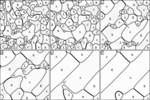
FIG. 1.: Temporal evolution of the extended-interaction-range model 5 under the phase transformation A1$\to$L1₀ shown in the $\eta^{2}$-representation for the simulation box size $V_{b}=128^{2}\times 1$ at the maximum tetragonal distortion parameter $|\varepsilon_{m}|=0.1$, $c=0.5$, the reduced temperature $T^{\prime}=T/T_{c}=0.7$, and the following values of the reduced time $t^{\prime}=t\gamma_{nn}$: (a) 10; (b) 20; (c) 50; (d) 100; (e) 250; and (f) 280. The grey level linearly varies with $\eta_{i}^{2}=\eta_{1i}^{2}+\eta_{2i}^{2}+\eta_{3i}^{2}$ between its minimum and maximum values from completely dark to completely bright. The symbol A, $\overline{{\rm A}}$, B, $\overline{\rm B}$, C or $\overline{\rm C}$ indicates the type of the ordered domain as described in the text. The thick, the thin and the single arrow indicates the fusion-of-domain process, the quadruple junction of APDs, and the splitting APB process, respectively, discussed in the text.

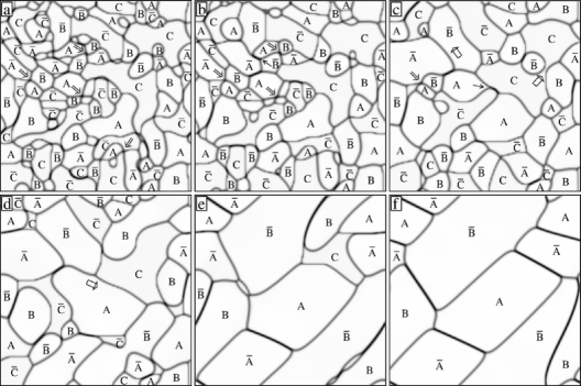
FIG. 2.: As figure 1, but for the intermediate-interaction-range model 4 at $T^{\prime}=0.67$ and the following values of $t^{\prime}$: (a) 10; (b) 20; (c) 50; (d) 100; (e) 250; and (f) 500.

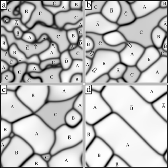
FIG. 3.: As figure 2, but at $T^{\prime}=0.92$ and the following values of $t^{\prime}$: (a) 10; (b) 50; (c) 100; and (d) 200.

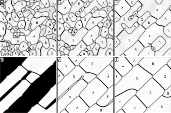
FIG. 4.: As figure 1, but at $|\varepsilon_{m}|=0.15$ and the following values of $t^{\prime}$: (a) 10; (b) 20; (c) 50; (d) 150; (e) 172; and (f) 350. Frame 2d is shown in the $\eta_{2}^{2}$-representation: the grey level linearly varies with $\eta_{2i}^{2}$ between its minimum and maximum values from completely dark to completely bright.

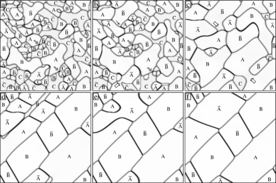
FIG. 5.: As figure 2, but at $|\varepsilon_{m}|=0.15$ and the following values of $t^{\prime}$: (a) 10; (b) 20; (c) 50; (d) 170; (e) 200; and (f) 300.

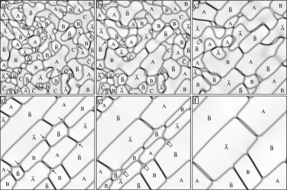
FIG. 6.: As figure 5, but at $c=0.44$ and the following values of $t^{\prime}$: (a) 10; (b) 20; (c) 50; (d) 400; (e) 750; and (f) 1100.

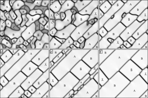
FIG. 7.: As figure 1, but at $|\varepsilon_{m}|=0.2$, $T^{\prime}=0.88$ and the following values of $t^{\prime}$: (a) 10; (b) 20; (c) 30; (d) 50; (e) 300; and (f) 400.

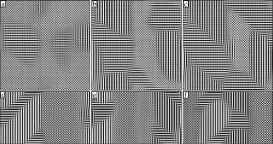
FIG. 8.: As figure 3, but for 3D simulation with $V_{b}=52^{2}\times 30$ at $|\varepsilon_{m}|=0.2$ and shown in the ‘$c$-representation’: the grey level linearly varies with $c_{i}$ between its minimum and maximum values from completely dark to completely bright. The three upper frames correspond to the plane $z=10\,a$ and the following values of $t^{\prime}$: (a) 10; (b) 20; and (c) 325. The three lower frames correspond to $t^{\prime}=325$ and the following planes: (d) $y=0$; (e) $y=10\,a$; and (f) $y=36\,a$.

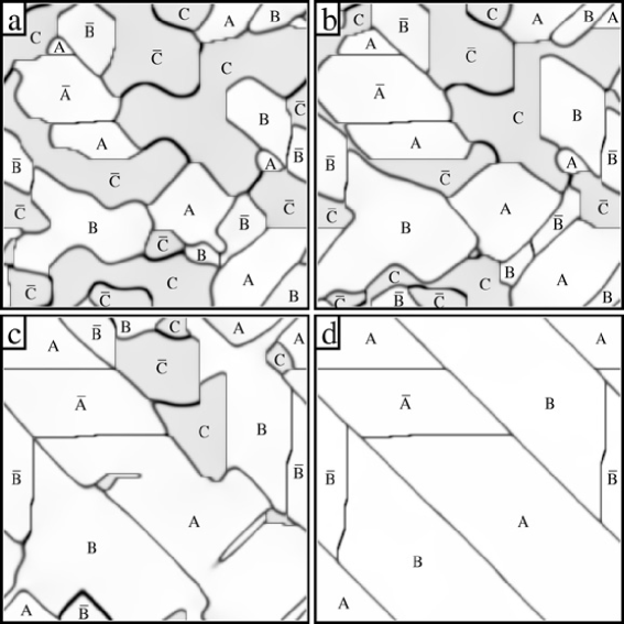
FIG. 9.: As figure 1 but for the short-range-interaction model 1 at $|\varepsilon_{m}|=0.15$, $c=0.5$, $T^{\prime}=0.9$ and the following values of $t^{\prime}$: (a) 30; (b) 40; (c) 60; and (d) 120.

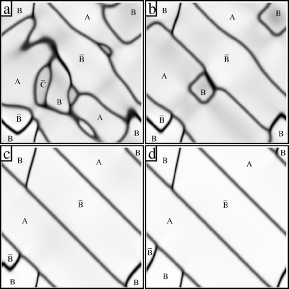
FIG. 10.: As figure 9 but at $c=0.44$ and the following values of $t^{\prime}$: (a) 110; (b) 140; (c) 200; and (d) 350.

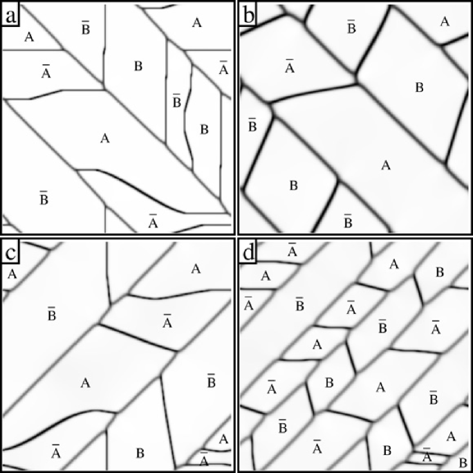
FIG. 11.: As figure 1 but for model $2$ at $|\varepsilon_{m}|=0.1$ and the following values of $c$, $T^{\prime}$ and $t^{\prime}$: (a) $c=0.5$, $T^{\prime}=0.77$, $t^{\prime}=350$; (b) $c=0.5$, $T^{\prime}=0.95$, $t^{\prime}=300$; (c) $c=0.46$, $T^{\prime}=0.77$, $t^{\prime}=350$; and (d) $c=0.44$, $T^{\prime}=0.77$, $t^{\prime}=300$.

REFERENCES

- [1] Present address: Ames Laboratory, Ames, IA 50011, USA.
- [2] Leroux C, Loiseau A, Broddin D and Van Tendeloo G 1991 Phil. Mag. B 64 57
- [3] Zhang B, Lelovic M and Soffa W A 1991 Scripta Met. 25 1577
- [4] Zhang B and Soffa W A 1992 Phys. Stat. Sol. (a) 131 707
- [5] Yanar C, Wiezorek J M K and Soffa W A 2000 Phase Transformations and Evolution in Materials ed P E A Turchi and A Gonis (Warrendale: The MMM Society) p 39
- [6] Tanaka Y, Udoh K-I, Hisatsune K and Yasuda K 1994 Phil. Mag. A 69 925
- [7] Oshima R, Yamashita M, Matsumoto K and Hiraga K 1994 Solid–Solid Phase Transformations ed W C Johnson et al.(Warrendale: The MMM Society) p 407
- [8] Syutkina V I, Abdulov R Z, Zemtsova N D and Yasyreva L P 1984 Fiz. Metal. Metalloved. 58 745
- [9] Roitburd A L 1968 Fiz. Tverd. Tela 10 3619 (Engl. Transl. 1969 Sov. Phys. Solid State 10 2870)
- [10] Khachaturyan A G and Shatalov G A 1969 Zh. Eksp. Teor. Fiz. 56 1037 (Engl. Transl. 1969 Sov. Phys.–JETP 10 557)
- [11] Khachaturyan A G 1983 Theory of Structural Phase Transformations in Solids (New York: Wiley)
- [12] Vaks V G 2001 Pis. Zh. Eksp. Teor. Fiz. 73 274 (Engl. Transl. 2001 JETP Lett. 73 237)
- [13] Chen L-Q, Wang Y Z and Khachaturyan A G 1992 Phil. Mag. Lett. 65 15
- [14] Vaks V G 1996 Pis. Zh. Eksp. Teor. Fiz. 63 447 (Engl. Transl. 1996 JETP Lett. 63 471)
- [15] Belashchenko K D and Vaks V G 1998 J. Phys.: Condens. Matter 10 1965
- [16] Belashchenko K D, Dobretsov V Yu, Pankratov I R, Samolyuk G D and Vaks V G 1999 J. Phys.: Condens. Matter 11 10593
- [17] Pankratov I R and Vaks V G 2001 J. Phys.: Condens. Matter 13 6031
- [18] Rouchy J and Waintal A 1975 Solid State Commun. 17 1227
- [19] Zunger A 1994 Statics and Dynamics of Alloy Phase Transformations (NATO Advanced Study Institute, Series B: Physics, vol 319) ed A Gonis and P E A Turchi (New York: Plenum) p 361
- [20] Beiden S V, Samolyuk G D, Vaks V G and Zein N E 1994 J. Phys.: Condens. Matter 6 8487
- [21] Berg H and Cohen J B 1972 Metall. Trans. 3 1797
- [22] Leroux C, Cadeville M C, Pierron-Bohnes V, Inden G and Hinz F 1988 J. Phys.: Met. Phys. 18 2033
- [23] Ducastelle F 1970 J. de Phys. 31 1055
- [24] Chassagne F, Bessiere M, Calvayrac Y, Cenedese P and Lefebvre S 1989 Acta Met. 37 2329
- [25] Vaks V G and Samolyuk G D 1999 Zh. Eksp. Teor. Fiz. 115 158 (Engl. Transl. 1999 Sov. Phys.–JETP 88 89)
- [26] Belashchenko K D, Samolyuk G D and Vaks V G 1999 J. Phys.: Condens. Matter 11 10567
- [27] Turchi P E A 1994 Intermetallic Compounds: Vol. 1, Principles, ed J H Westbrook and R L Fleicher (New York: Wiley) p 21
- [28] Potez L and Loiseau A 1994 J. Interface Sci. 2 91