Propagation-Dispersion Equation

Abstract

A propagation-dispersion equation is derived for the first passage distribution function of a particle moving on a substrate with time delays. The equation is obtained as the continuous limit of the first visit equation, an exact microscopic finite difference equation describing the motion of a particle on a lattice whose sites operate as time-delayers. The propagation-dispersion equation should be contrasted with the advection-diffusion equation (or the classical Fokker-Planck equation) as it describes a dispersion process in time (instead of diffusion in space) with a drift expressed by a propagation speed with non-zero bounded values. The temporal dispersion coefficient is shown to exhibit a form analogous to Taylor’s dispersivity. Physical systems where the propagation-dispersion equation applies are discussed.

I Introduction

Often to describe the microscopic mechanism of a diffusion process, one considers a test particle executing a random walk on some substrate, and one writes a mean-field equation in terms of the probabilities that the particle performs elementary displacements in given or arbitrary directions. The question one then asks is: where will the particle be after some given time (in the long-time limit)? The answer is given by the distribution function $F(r,t)$, the probability that, given the particle was initially at $r=0$ at $t=0$, it will be at position $r$ at time $t$ (for $t\rightarrow\infty$, that is for $t$ large compared to the duration of an elementary displacement). $F(r,t)$ is obtained as the solution to the Fokker-Planck equation for diffusion, and one finds that, in the the long-time limit, $F(r,t)$ is Gaussianly distributed in space feller .

When there is an interactive process between the particle and the substrate such that the particle undergoes directed motion subjected to time delays, it is interesting to view the motion in terms of first passages, and one expects that the long-time dynamics will be different from that described by the usual diffusion equation. We obtain indeed a new equation for the long-time behavior of the first visit distribution function $f(r,t)$ of a particle whose dynamics is governed by a distribution of time delays. The main results in this paper are (i) the propagation-dispersion equation

$${}\frac{\partial}{\partial r}f(r,t)\,+\,\frac{1}{c}\,\frac{\partial}{\partial t}f(r,t)\,=\,\frac{\gamma}{2}\,\frac{\partial^{2}}{\partial{t^{2}}}f(r,t)\;,$$

where $c$ is the propagation speed, and (ii) the expression for the time dispersion coefficient in terms of the covariance of the reciprocal velocity fluctuations

$${}\gamma\,=\,\xi\,\left(\langle\frac{1}{v^{2}}\rangle-\frac{1}{c^{2}}\right)\,,$$

where $\xi$ is a characteristic correlation length. We first give a heuristic derivation of the propagation-dispersion equation using multi-scale analysis which is then further substantiated by a more mathematically rigorous development. Using the latter method, we show that the above results generalize to inhomogeneous systems with $c\rightarrow c(r)$ and $\gamma\rightarrow\gamma(r)$.

A characteristic example where the equation applies is particle dispersion in a granular medium as studied experimentally by Ippolito et al. hulin , as we shall discuss below. On the other hand, there are prototypical abstract systems, for particle-substrate interactive dynamics, such as the automaton known as Langton’s ant ant and other simple automata cohen ; grosfils , where particle-substrate interactions produce time delays in the dynamics. These automaton systems offer the advantage of explicit microscopic dynamics which can be solved exactly. For instance Grosfils, Boon, Cohen, and Bunimovich grosfils developed a one-dimensional automaton for which they provided a mathematical analysis also applicable to the two-dimensional triangular lattice.

The one-dimensional case is particularly simple to describe. The automaton universe is the one-dimensional lattice where, at each time step, a particle moves from site to site, in the direction given by an indicator. One may think of the indicator as a ‘spin’ ($\uparrow$ or $\downarrow$) defining the state of the site: when the particle arrives at a site with spin up, it moves to the next neighboring site in the direction of its incoming velocity vector, whereas its velocity is reversed if the spin is down. But the particle modifies the state of the visited site ($\uparrow\Longleftrightarrow\downarrow$) so that on its next visit, the particle is deflected in the direction opposite to the scattering direction of its former visit. With this specific microscopic dynamics, back-scattering produces time delay. Grosfils et al. derived the equations describing the microscopic dynamics of the particle on the one-dimensional lattice (and also on the triangular lattice) under the general condition that the spins at the initial time can be arbitrarily distributed. They proved that the particle will always go into a propagation phase, regardless of the initial distribution of spins; they also showed that the basic mechanism for propagation is a blocking process grosfils .

It was shown by Boon boon that the propagation equations in grosfils are particular cases of a general equation describing the first visit of the particle to a new site in the propagation phase. This equation, obtained in the context of specific lattice dynamics, is a first passage equation which has more general applicability, and will be our starting point in the present work.

II First visit equation

Consider a particle propagating in a D-dimensional channel; we project its motion onto a one-dimensional lattice - the propagation line - whose sites are labeled by integers $l=0,\,1,\,2,\,...\,$. The distance, in lattice units, between neighboring sites on the propagation line is denoted by $\delta r$. We set the clock at $t_{0}=0$ when the particle is at site $l=0$ where it enters the propagation channel. Its trajectory will intercept successively sites $l=1,\,2,\,3,\,...$ for the first time at times $t_{1},\,t_{2},\,t_{3}\,...$ respectively. The $t_{i}$’s are integer multiples of the automaton time step $\delta t$. While sites $0,\,1,\,2,\,3,\,...$ are equally spaced, the time differences between first visits, $t_{i+1}-t_{i}$, are (in general) not equally distributed.

A given (arbitrary) spin configuration defines a set of first passage times $t_{1},\,t_{2},\,...\,$. Let $i_{r}$ be the random variable which corresponds to the number of steps required for the particle to reach position $r=l_{r}\delta r$ for the first time. We define $f(r,t)$ as the probability of finding the particle at position $r$ for the first time at time $t=t_{r}=i_{r}\delta t$; $f(r,t)$ obeys the first visit equation, i.e. the finite difference equation boon

$$f(r,t)=\sum_{j=0}^{n}\,p_{j}\,f(r-\delta r,t-\tau_{j})\;.$$ (1)

Here $p_{j}$ is the probability that the particle propagates from $r-\delta r$ to $r$ in $\tau_{j}/\delta t$ time steps, i.e. $\tau_{j}$ is the time between two successive first visits on the propagation line. The sum is over all possible time delays, weighted by the probability $p_{j}$ with $\sum_{j=0}^{n}\,p_{j}\,=\,1$. For specific lattice dynamics, this is a condition for the existence of a blocking mechanism (described in grosfils ) responsible for propagation, and an explicit expression can then be given for $\tau_{j}$ (see Appendix). Here we present a general derivation for which this specification is not necessary.

An alternative equivalent formulation of Eq.(1) reads

$$f(r,t)=\sum_{j=0}^{\infty}\,{\tilde{p}}_{j}\,f(r-\delta r,t-j\delta t)\;,$$ (2)

which we shall use in Section VI. The difference between the two formulations is that the structure of the distribution of the delays is contained either in the $\tau_{j}$’s (Eq.(1)) or in the ${\tilde{p}}_{j}$’s (Eq.(2)).

Equation (1) - or equivalently (2) - expresses the probability that the particle be for the first time at position $r$ at time $t$ in terms of the probability that it was visiting site $r-\delta r$ at earlier time $t-\tau_{j}$, where $j=0,1,2,...,n$. Given a site $r$ on the propagation line, the particle will infallibly reach that site in the course of its displacements; the question then is: when will the particle be at position $r$ when $r$ is large? Since the particle executes $t/\delta t$ displacements to cover the distance $r$, the answer will be given in terms of the time distribution of the probability $f(r,t)$ for large fixed value of $r$, i.e. for $l_{r}\gg 1$. This corresponds to taking the continuous limit of equation (1) in a physically consistent way that we establish in Section III and in a mathematically rigorous way as shown in Section VI.

For one particular realization, the successive time delays are set by a given spatial configuration of the time delayers, and the time taken by the particle to perform a displacement from $r-\delta r$ to $r$ depends on that configuration. For an ensemble of realizations, the distribution function of the time delays defines the average displacement time

$$\langle\tau\rangle\,=\,\sum_{j=0}^{n}\,\,p_{j}\,\tau_{j}\,=\,\sum_{j=0}^{n}\,\mu_{j}\,p_{j}\,\delta t\,=\,\langle\mu\rangle\,\delta t\;,$$ (3)

and the variance

$$\langle\tau^{2}\rangle-\langle\tau\rangle^{2} = \left\{\sum_{j=0}^{n}\mu_{j}^{2}\,p_{j}\,-[\sum_{j=0}^{n}\mu_{j}\,p_{j}]^{2}\right\}\,(\delta t)^{2}$$ (4)

$$= (\langle\mu^{2}\rangle-\langle\mu\rangle^{2})\,(\delta t)^{2}\;,$$

where $\mu_{j}=\tau_{j}/\delta t$ is the number of time steps during the time delay $\tau_{j}$. The general condition on the $p_{j}$ distribution is that its moments be finite (for specific lattice dynamics, such as described in the Appendix, they are finite by virtue of the blocking mechanism discussed in grosfils ). Higher order moments $\langle\tau^{a}\rangle$ are defined similarly.

III Multi-scale analysis

Here we discuss how the continuous limit should be taken given that the system exhibits two time scales which correspond to (i) a propagation process characterized by the average time necessary to complete a finite number of displacements $r/\delta r$

$${\rm E}[t_{r}]\,=\,\langle\mu\rangle\,r\,\frac{\delta t}{\delta r}\;,$$ (5)

and (ii) the dispersion around this average value characterized by the variance

$${\rm Var}[t_{r}]\,=\,(\langle\mu^{2}\rangle\,-\,\langle\mu\rangle^{2})\,(\delta t)^{2}\,\frac{r}{\delta r}\;.$$ (6)

For finite $r$, these are finite quantities. Correspondingly we define the following quantitites that will be used in the continuous limit

$$\frac{1}{c}\,=\,\langle\mu\rangle\,\frac{\delta t}{\delta r}\;,$$ (7)

and

$$\gamma\,=\,(\langle\mu^{2}\rangle\,-\,\langle\mu\rangle^{2})\,\frac{(\delta t)^{2}}{\delta r}\;.$$ (8)

$c$ ($\neq 0$) will be identified as the propagation speed (see Section IV) and $\gamma$ ($\geq 0$) will be identified as the dispersion coefficient (see Section V).

We want to compute the continuous limit of the first visit equation (1), and obtain a partial differential equation for $f(r,t)$. The procedure must be performed in two successive steps according to the scale over which one wants to probe the process when $r$ is large. This is analogous to multi-scale expansion in the derivation of the Fokker-Plank equation kampen or of the Navier-Stokes equation multiscale . Consider that, to measure first passages, we use a detector with tunable resolution. The first visit time $t_{r}$ goes like $r$ (see (5)); so in order that the measure be performed with the same accuracy at any position $r$, we need a resolution such that $t_{r}/r$ has always the same order of magnitude. We can then measure first visit times at any position $r$ with a resolution which is appropriate to evaluate the average first passage time, i.e. to measure the propagation speed $c$. However, when performing measurements over many realizations, the successive arrival times at position $r$ (the fluctuations around the average time) will be poorly resolved (see insets in Fig.1). In order to measure the dispersion around ${\rm E}[t_{r}]$ with sufficient accuracy, the detector must be adjusted so that dispersion measurements at various positions $r$ can be performed with the same resolution. Therefore we impose that the width $\Delta T\,=\,\sqrt{{\rm Var}[t_{r}]}$ of the dispersion curve be measured with a resolution $\delta T$ such that the curve always contains about the same number of points, i.e. $\Delta T/\delta T$ has the same order of magnitude for all positions. Since $\Delta T$ grows with the distance like $\sqrt{r}$ (see (6)), $\delta T$ must also go $\sim\sqrt{r}$ in order to obtain an acurate measure of the dispersion $\gamma$ (see (8)).

We may summarize by saying that the continuous limit must be taken in a sequential order, first to obtain the average first passage time (which gives a measure of the propagation velocity $c$), and second, to measure the first passage dispersion in the moving reference frame (i.e. around $E[t_{r}]$). The first step will yield an Euler type equation and the second step the propagation-dispersion equation. Mathematically, these two steps materialize in the two successive orders, ${\cal O}(\epsilon^{1})$ and ${\cal O}(\epsilon^{2})$, of the development in Section IV, where $\epsilon$ is a smallness parameter defined as $\delta t/t_{obs}$, the ratio of the microscopic time to the macroscopic observation time. The continuous limit corresponds to $\epsilon\ll 1$. It follows from the above discussion that there are two length scales: (i) the first one corresponds to propagation

$$t_{obs}\,c\,=\,t_{obs}\frac{1}{\langle\mu\rangle}\frac{\delta r}{\delta t}\,=\,\langle\mu\rangle^{-1}\epsilon^{-1}\delta r\,,$$ (9)

for which the measurement unit is $\epsilon^{-1}\delta r$; (ii) the second length scale corresponds to dispersion

$$t_{obs}^{2}\,\frac{1}{\gamma}\,=\,t_{obs}^{2}\,\frac{1}{\langle\mu^{2}\rangle-\langle\mu\rangle^{2}}\frac{\delta r}{(\delta t)^{2}}\,=\,(\langle\mu^{2}\rangle-\langle\mu\rangle^{2})^{-1}\epsilon^{-2}\delta r\,,$$ (10)

which is thus measured in units $\epsilon^{-2}\delta r$. It is therefore natural to introduce two space variables, $r_{1}\,=\,\epsilon r$ and $r_{2}\,=\,\epsilon^{2}r$, and correspondingly two time variables, $t_{1}\,=\,\epsilon t$ and $t_{2}\,=\,\epsilon^{2}t$. Note that $r_{1}$ and $r_{2}$ are merely two expressions of the space variable $r$ with different scalings, and similarly for $t_{1}$ and $t_{2}$. Consequently the space and time derivative operators must be rescaled as

$$\partial_{r}\rightarrow\epsilon\partial_{r_{1}}\,+\,\epsilon^{2}\partial_{r_{2}}\;\;\;;\;\;\;\partial_{t}\rightarrow\epsilon\partial_{t_{1}}\,+\,\epsilon^{2}\partial_{t_{2}}$$ (11)

Accordingly $f(r,t)$ is expanded as $f\,=\,f^{(0)}\,+\,\epsilon f^{(1)}\,+\,\,{\cal O}(\epsilon^{2})$, where $f^{(0)}$ is the distribution function in the absence of dispersion ($f^{(0)}$ plays the same role as the local equilibrium distribution function in the derivation of the Navier-Stokes equation multiscale ).

While in taking the continuous limit, there is a mathematical separation of scales (i.e. one probes either the propagation mode or the dispersion mode), in practice, there are systems with sufficiently large $\gamma$ (see Section VII and Appendix) where propagation and dispersion can be measured simultaneously, provided one uses a detector with high resolution.

IV Propagation-dispersion equation

In order to compute the continuous limit of Eq.(1), it is convenient to rewrite the equation as

$$f(r+\delta r,t)=\sum_{j=0}^{n}\,p_{j}\,f(r,t-\tau_{j})\;,$$ (12)

to which we now apply the multi-scale expansion (in Section VI we give an alternative derivation which is more mathematically rigorous).

To first order, we obtain

$${\cal O}(\epsilon^{1}):\;\;\;\;\partial_{r_{1}}f^{(0)}\,=\,-\frac{\langle\tau\rangle}{\delta r}\,\partial_{t_{1}}f^{(0)}\,=\,-\langle\mu\rangle\frac{\delta t}{\delta r}\,\partial_{t_{1}}f^{(0)}\;,$$ (13)

or, with (7),

$$\partial_{r_{1}}f^{(0)}\,+\,\frac{1}{c}\,\partial_{t_{1}}f^{(0)}\,=\,0\;,$$ (14)

which is an Euler equation.

To second order, we have

$${\cal O}(\epsilon^{2}):\;\;\;\;\partial_{r_{2}}f^{(0)}\,+\,\partial_{r_{1}}f^{(1)}\,+\,\frac{1}{2}\delta r\,\partial_{r_{1}}^{2}f^{(0)} =$$

$$-\,\frac{\langle\tau\rangle}{\delta r}\,(\partial_{t_{2}}f^{(0)}\,+\,\partial_{t_{1}}f^{(1)})\, + \,\frac{1}{2}\frac{\langle\tau^{2}\rangle}{\delta r}\,\partial_{t_{1}}^{2}f^{(0)}\;,$$ (15)

where we will inject the first order result (13). This substitution can be performed either in the last term on the l.h.s. or in the last term on the r.h.s. with two different results of which only one can be correct. In fact there is no ambiguity as to which is the legal procedure: Eq. (12) is local in space (not in time) which indicates that in the continuous limit we must obtain a partial differential equation with a spatial derivative not exceeding first order. The correct substitution of (13) into (IV) gives

$$\partial_{r_{2}}f^{(0)}\,+\,\partial_{r_{1}}f^{(1)}\,=\,-\frac{1}{c}\,(\partial_{t_{2}}f^{(0)}\,+\,\partial_{t_{1}}f^{(1)})\,+\,\frac{1}{2}\left(\frac{\langle\tau^{2}\rangle}{\delta r}\,-\,\frac{\delta r}{c^{2}}\right)\,\partial_{t_{1}}^{2}f^{(0)}\;,$$ (16)

where the quantity in parantheses in the second term of the r.h.s. is equal to $(\langle\mu^{2}\rangle\,-\,\langle\mu\rangle^{2})(\delta t)^{2}/{\delta r}\equiv\gamma$.

Summing Eqs.(14) and (16) after multiplication by $\epsilon$ and by $\epsilon^{2}$ respectively, we obtain

$$\epsilon\,\partial_{r_{1}}(f^{(0)}+\epsilon\,f^{(1)})\,+\epsilon^{2}\,\partial_{r_{2}}\,f^{(0)}=\,-\frac{1}{c}\,\epsilon\,\partial_{t_{1}}(f^{(0)}+\epsilon\,f^{(1)})\,-\,\frac{1}{c}\,\epsilon^{2}\,\partial_{t_{2}}\,f^{(0)}+\frac{\gamma}{2}\,\epsilon^{2}\,\partial_{t_{1}}^{2}\,f^{(0)}\,.$$ (17)

Rearranging terms (incorporating terms of negligible higher order) and going back to the original variables yields

$$\partial_{r}\,f(r,t)\,+\,\frac{1}{c}\,\partial_{t}f(r,t)\,=\,\frac{1}{2}\,\gamma\,\partial_{t}^{2}f(r,t)\;,$$ (18)

where terms of order $\epsilon>2$ are omitted. With the initial condition that at the origin, say at $r=0$, $f(0,t)\,=\,\delta(t)$, the solution to Eq.(18) is

$$f(r,t)\,=\,\sqrt{\frac{1}{2\pi}}\,(\gamma\,r)^{-\frac{1}{2}}\exp\,\left(-\,\frac{(t\,-\,\frac{r}{c})^{2}}{2\,\gamma\,r}\right)\;.$$ (19)

These results are confirmed by the more mathematically rigorous derivation given in Section VI. Note that in the case that all $p_{j}$’s are zero except one ($\mu_{j}\equiv\mu$, e.g. for Langton’s ant), then $\gamma\,=\,0$, and (18) reduces to the Euler equation (14) with $c\,=\,{\delta r}/(\mu\,\delta t)$ (see boon ).

It is clear from (18), that $c$ is a propagation speed, and $\gamma$ is a transport coefficient expressing dispersion in time (instead of space like in the classical Fokker-Planck equation for diffusion). Equation (18) is the propagation-dispersion equation governing the first-passage distribution function of a propagating particle subject to time delays. Propagation is guaranteed because $c$ is non-zero ($\langle\mu\rangle$ is finite); $c$ has a finite maximum value for $n=0$ (i.e. $j=0$ and $p_{0}=1$), in which case $\gamma=0$ (see (4)), and there is propagation without dispersion.

In Fig.1 we show that the above analytical results are in perfect agreement with the numerical solution of the general equation, Eq.(1). We used delay times equally distributed (Fig.1a) and exponentially distributed (Fig.1b); explicit values of the quantities $c$ and $\gamma$ are given in the figure caption.

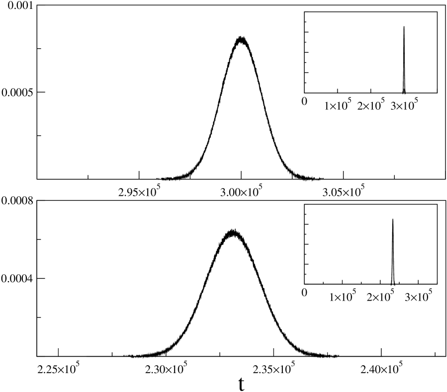
Figure 1: Probability distribution $f(r=3\times 10^{4},\,t)$ based on general equation (1). Here $\mu_{j}\,=\,1+2j$, so $c=[(1+2\langle j\rangle)]^{-1}$. (a) time delays equally distributed for $j\,=0,\,1,\,\cdots,\,9$, with $p_{j}\,=\,0.1$; $c=0.1$ and $\gamma=33$; half-width $=\sqrt{2\gamma r}\simeq 1.41\times 10^{3}$. (b) time delays exponentially distributed: $p_{j}\,=\,C\,\exp{-\beta j}$, with $j=0,\,1,\,...,\,9$, $\beta\,=\,0.25$, and $C\,=\,[\sum_{j=0}^{9}j]^{-1}=1/45$; $c=0.128$ and $\gamma=52.7$; half-width $=\sqrt{2\gamma r}\simeq 1.78\times 10^{3}$. The numerical simulation data and the analytical expression (Eq.(19); solid line, not visible) coincide perfectly. Insets: see text. In this and subsequent figures, time unit is the automaton time step.

V Dispersion and correlations

(i)The dispersion coefficient. It follows from Eqs.(6) and (8), that $\gamma$ is given by

$$\gamma\,=\,\frac{\langle t_{r}^{2}\rangle-\,\langle t_{r}\rangle^{2}}{r}\,$$ (20)

which, for large $r$, is reminiscent of the classical expression for the diffusion coefficient: $D\,=\,\lim_{t\to\infty}\langle r^{2}(t)\rangle/2t$. Comparison of the two expressions shows interchange of space and time, a feature which is illustrated in Figs.2 and 3. In Fig.2, we show three typical runs on the 1-D spin-lattice by plotting the first passage time (minus the mean time of arrival $\langle t_{r}\rangle=r/c$) as a function of distance $r$. One observes that $[t-\langle t_{r}\rangle]$ as a function of $r$ exhibits fluctuations of the same nature as those obtained when plotting the position of a random walker as a function of time. In Fig.3 we present simulation data illustrating Eq.(20). From measurements performed in the 1-D lattice, the variance $\langle t_{r}^{2}\rangle-\,\langle t_{r}\rangle^{2}$ is seen to be a linear function of distance (see inset) with a slope equal to $\gamma$ (main frame) in the same way as the diffusion coefficient is obtained as the slope of the mean-square displacement versus time in the long-time limit of the classical random walk.

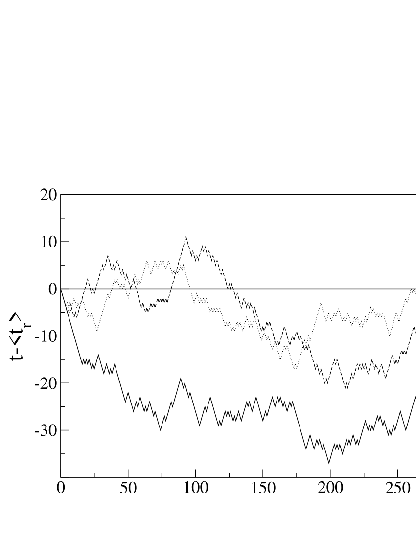
Figure 2: Displacement time $(t-\langle t_{r}\rangle\,=\,t-r/c)$ as a function of distance $r$ for three different realizations in the 1-D lattice (see Appendix: $q=.5$, and $j=0,1$). Vertical axis: time in automaton time steps; horizontal axis: distance in lattice unit lengths.

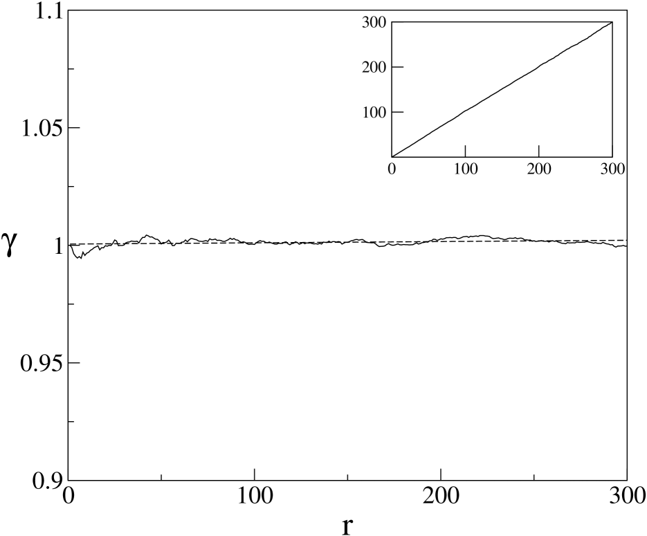
Figure 3: Dispersion coefficient, see Eq.(20), in $1-$D lattice (see Appendix: $q=0.5,\,j=0,1,\,p_{0}=q,\,p_{1}=1-q,$ and $\mu_{j}=1+2j$). Inset shows $\langle t_{r}^{2}\rangle\,-\,\langle t_{r}\rangle^{2}$ as a function of $r$, for one single realization, and main frame shows $\gamma$ measured from the slope in inset; the horizontal dashed line is the theoretical value: $\gamma=(\langle\mu^{2}\rangle\,-\,\langle\mu\rangle^{2})=q+(1-q)3^{2}\,-\,(3-2q)^{2}=4q(1-q)=1$. $r$ is in lattice unit lengths and $\gamma$ is in automaton time steps squared per lattice unit length.

(ii) The correlation function. From Eqs.(5) and (7), we have $\frac{1}{c}\,=\,\frac{\langle t_{r}\rangle}{r}$. Here $t_{r}$ can be expressed in terms of the local propagation velocity $v(r)$, a fluctuating quantity with average value $c$. In fact it is the reciprocal local velocity which is physically relevant: it is the time taken by the particle to propagate from position $r$ to $r+\delta r$ (divided by $\delta r$). Then indeed

$$\langle t_{r}\rangle\,=\,\langle\int_{0}^{r}\,dr^{\prime}\,\frac{1}{v(r^{\prime})}\,\rangle\,=\,\int_{0}^{r}\,dr^{\prime}\,\langle\frac{1}{v(r^{\prime})}\,\rangle\,=\,\frac{r}{c}\,,$$ (21)

which is consistent with the definition of the propagation speed.

Expressing the time $t_{r}$ in terms of the local velocity $v(r)$, we have

$$\langle t_{r}^{2}\rangle\,=\,\langle\int_{0}^{r}\,dr^{\prime}\,\frac{1}{v(r^{\prime})}\,\int_{0}^{r}\,dr^{\prime\prime}\,\frac{1}{v(r^{\prime\prime})}\rangle\,=\,\int_{0}^{r}\,dr^{\prime}\,\int_{0}^{r}\,dr^{\prime\prime}\langle\frac{1}{v(r^{\prime})}\,\frac{1}{v(r^{\prime\prime})}\rangle\,,$$ (22)

and

$$\langle t_{r}^{2}\rangle-\langle t_{r}\rangle^{2} = \int_{0}^{r}\,dr^{\prime}\,\int_{0}^{r}\,dr^{\prime\prime}\langle\left(\frac{1}{v(r^{\prime})}-\langle\frac{1}{v}\rangle\right)\,\left(\frac{1}{v(r^{\prime\prime})}-\langle\frac{1}{v}\rangle\right)\rangle\,.$$ (23)

In terms of the reciprocal velocity fluctuations $\delta v^{-1}(r)=v^{-1}(r)-\langle v^{-1}\rangle=v^{-1}(r)-c^{-1}$, (23) reads

$$\langle t_{r}^{2}\rangle-\langle t_{r}\rangle^{2} = \int_{0}^{r}\,dr^{\prime}\,\int_{0}^{r}\,dr^{\prime\prime}\langle\delta v^{-1}(r^{\prime})\,\delta v^{-1}(r^{\prime\prime})\rangle\,.$$ (24)

The dynamics of the propagating particle implies that the correlation function on the r.h.s. of (24) is $\delta$-correlated, i.e. $\langle\delta v^{-1}(r^{\prime})\,\delta v^{-1}(r^{\prime\prime})\rangle\,=\,\phi_{0}\,\delta(\frac{r^{\prime}}{\xi}-\frac{r^{\prime\prime}}{\xi})$ with $\phi_{0}\,=\,\langle(\delta v^{-1})^{2}\rangle\,=\,\langle\frac{1}{v^{2}}\rangle-\frac{1}{c^{2}}$, and where $\xi$ is the elementary correlation length. So it follows from (20) and (24) that

$${\gamma}\,=\,\xi(\langle v^{-2}\rangle-c^{-2})\,,$$ (25)

that is ${\gamma}$ is the covariance of the reciprocal velocity fluctuations multiplied by the correlation length (here equal to one lattice unit length). This result is analogous to Taylor’s formula of hydrodynamic dispersivity which is expressed as the product of the covariance of the velocity fluctuations with a characteristic correlation time taylor . We call $\gamma$ the temporal dispersion coefficient. Evidently, there is no dispersion ($\gamma=0$) in the absence of velocity fluctuations ($\phi_{0}\,=\,0$).

From these results, the explicit computation of the dispersion coefficient is straightforward. For instance for the one-dimensional spin-lattice (see Appendix; Fig.4a), the local velocity is either $1$, with probability $q$, or $1/3$, with probability $(1-q)$, and the reciprocal mean velocity is $c^{-1}\,=\,q\,+\,3(1-q)$; so

$${\gamma}\,=\,q\,+\,3^{2}(1-q)-c^{-2}\,=\,4q(1-q)\,,$$ (26)

which is exactly the value of $\gamma$ evaluated for the 1-D spin lattice in the Appendix and in grosfils . A similar computation for the triangular lattice (see Fig.4b) yields the value $\gamma=72q(1-q)$ in accordance with the result obtained in grosfils .

(iii) The time current. Writing Eq.(18) as

$$(\partial_{r}\,+\,\frac{1}{c}\,\partial_{t})\,f(r,t)\,+\,\partial_{t}\,j(r,t) = 0\;,$$ (27)

with $j(r,t)=-\frac{\gamma}{2}\,\partial_{t}\,f(r,t)$, shows formal analogy with the classical mass conservation equation

$$(\partial_{t}\,+\,{\bf c}\cdot\nabla)\,\rho({\bf r},t)\,+\,\nabla\cdot{\bf j}({\bf r},t) = 0\;,$$ (28)

with space and time variables interchanged. So in (27), $j(r,t)$ can be interpreted as a “current in time ”.

(iv) The control parameter. In classical advection-diffusion phenomena, the control parameter is the Péclet number $P=UL/2D$, where $U$ denotes the mean advection speed, $L$, the characteristic macroscopic length, and $D$, the diffusion coefficient (see e.g. koplik ). The analogue for propagation-dispersion follows by casting Eq.(18) in non-dimensional form

$$\partial_{\tt r}\,f(r,t)\,+\,\partial_{\tt t}\,f(r,t)\,=\,B^{-1}\,\partial_{\tt t}^{2}\,f(r,t)\;;\;\;\;\;B=\frac{2T}{\gamma c}\;.$$ (29)

Here ${\tt r}$ and ${\tt t}$ are the dimensionless space and time variables: ${\tt r}=r(cT)^{-1}$ and ${\tt t}=t\,T^{-1}$, where $T$ is a characteristic macroscopic time. $B$ is the control parameter for propagation-dispersion: it is a measure of the relative importance of propagation with respect to dispersion. Indeed, $B=\frac{2T}{\gamma c}=\frac{2T^{2}}{\gamma}\frac{1}{cT}=L_{D}/L_{P}$, i.e. the ratio of the characteristic dispersion length $L_{D}$ to the characteristic propagation length $L_{P}$. At high values of $B$, i.e. $L_{D}\gg L_{P}$, the distribution function is very narrow, and transport over large distances ($r\geq cT$) is dominated by propagation.

(v) The power spectrum. The propagation-dispersion equation (18), subject to the initial condition $f(r=0,t)\,=\,\delta(t)$, describes an initial value problem with initial value fixed in space; so we can solve the equation by spatial Laplace transformation. Using $\kappa$ as the conjugate space variable, we obtain

$$\kappa\,{\tilde{f}}(\kappa,\omega)\,-\,f(r=0,\omega)\,=\,-\frac{\imath\,\omega}{c}\,{\tilde{f}}(\kappa,\omega)\,-\,\frac{\gamma}{2}\,\omega^{2}\,{\tilde{f}}(\kappa,\omega)\;,$$ (30)

where $f(\omega)$ denotes the time Fourier transform. With the initial condition $f(r=0,t)=\delta(t)$, i.e. $f(r=0,\omega)=\frac{1}{2\pi}$, (30) yields

$${\tilde{f}}(\kappa,\omega)\,=\,\frac{1}{2\pi}\,(\,\kappa\,+\,\,\frac{\imath\,\omega}{c}\,+\,\frac{\gamma}{2}\,\omega^{2}\,)^{-1}\;.$$ (31)

This result shows that the system dynamics is described by one single mode: $\kappa\,=\,-\,\frac{\imath\,\omega}{c}\,-\,\frac{\gamma}{2}\,\omega^{2}$. The corresponding spectrum $S(k,\omega)\,=\,2\,Re\,{\tilde{f}}(\kappa=\imath\,k,\omega)$ is given by

$$S(k,\omega)\,=\,\frac{1}{2\pi}\,\frac{\gamma\,\omega^{2}}{(k\,+\,\omega\,/c\,)^{2}\,+\,\frac{1}{4}\,(\gamma\,\omega^{2}\,)^{2}}\;,$$ (32)

with $\int_{0}^{\infty}S(k,\omega)\,dk=1$. The spectrum (32) (which can also be obtained by double Fourier transformation of (19)) exhibits a single Lorentzian line typical of a diffusive phenomenon, but there are two essential differences with the spectrum obtained from the classical advection-diffusion equation: (i) the spectrum is a Lorentzian in $k$ (rather than in $\omega$) with half-width at half-height $\Delta k=\frac{1}{2}\gamma\omega^{2}$, indicating that dispersion is diffusive in time (instead of space); (ii) the Lorentzian is shifted by a quantity proportional to the reciprocal of the propagation speed.

VI Exact solution of the first-visit equation

In order to emphasize the discrete nature of the problem, we introduce the notation

$$g(l,i)=\left(\delta t\right)f(l\delta r,i\delta t),$$ (33)

where here, and below, latin arguments ($l,i,j,\cdots$) always indicate integers. The first visit equation, Eq.(2), is then

$$g(l,i)=\sum_{j=0}^{\infty}{\tilde{p}}_{j}^{\left(l-1\right)}g(l-1,i-j)\,.$$ (34)

Here we consider the general case where the transition probabilities $p_{j}^{(l)}$ depend on the lattice position $l$ as indicated by the superscript (for simplicity we omit the tilde notation). It is convienient to introduce the generating function for the distribution which is defined to be

$$h_{l}(x)\equiv\sum_{i=0}^{\infty}x^{i}g(l,i),$$ (35)

and from which the distribution is obtained via

$$g(l,i)=\lim_{x\rightarrow 0}\frac{1}{i!}\frac{d^{i}}{dx^{i}}h_{l}(x).$$ (36)

Temporal moments of the distribution can be calculated as

$$\left\langle j^{a}\right\rangle=\sum_{j=0}^{\infty}j^{a}g\left(l,j\right)=\lim_{z\rightarrow 0}\frac{d^{a}}{dz^{a}}h_{l}(e^{z})\,,$$ (37)

so that $M_{l}(z)=h_{l}(e^{z})$ is the generating function for moments of the first passage time at lattice position $l$. The boundary condition that the particle starts at lattice site $l=0$ at time $i=0$ implies that $g(0,i)=\delta_{i0}$, or equivalently $h_{0}(x)=1$.

Substituting Eq.(34) into Eq.(35) gives

$$h_{l}(x) \equiv \sum_{i=0}^{\infty}x^{i}\sum_{j=0}^{\infty}p_{j}^{\left(l-1\right)}g(l-1,i-j)$$ (38)

$$= h_{l-1}(x)\sum_{j=0}^{\infty}p_{j}^{\left(l-1\right)}x^{j},$$

so that the general solution is

$$h_{l}(x)\,=\,h_{0}(x)\,\prod_{k=1}^{l}\left(\sum_{j=0}^{\infty}p_{j}^{\left(k-1\right)}x^{j}\right)\,.$$ (39)

Using this solution and Eq.(37), exact moments may be easily calculated; with the normalization $\sum_{j=0}^{\infty}p_{j}^{(k)}=1$, we obtain

$$\left\langle j;l\right\rangle = l\,\langle\mu\rangle_{l}\,,$$ (40)

$$\left\langle j^{2};l\right\rangle-\left\langle j;l\right\rangle^{2} = l\sigma_{l}^{2}\,,$$ (41)

where

$$\langle\mu\rangle_{l} = \frac{1}{l}\sum_{k=1}^{l}\sum_{j=0}^{\infty}p_{j}^{\left(k-1\right)}j\,,$$ (42)

$$\sigma_{l}^{2} = \frac{1}{l}\sum_{k=1}^{l}\left[\sum_{j=1}^{\infty}p_{j}^{\left(k-1\right)}j^{2}-\left(\sum_{j=1}^{\infty}p_{j}^{\left(k-1\right)}j\right)^{2}\right]\,,$$ (43)

are just averages over the elementary process. In order to develop the limiting form of the distribution for large $l$, we assume that $\langle\mu\rangle_{l}$ and $\sigma_{l}^{2}$ are of order $1$ for all $l$ as is certainly true if the elementary probabilities are independent of lattice position. We then introduce a new stochastic variable which measures deviations away from the expected waiting time as

$$w_{l}=\frac{\left(j-l\langle\mu\rangle_{l}\right)}{\sqrt{l\sigma_{l}^{2}}}\,.$$ (44)

The moment generating function $N_{l}(z)$ for this new variable is related to that for the original variable by

$$N_{l}(z)=\exp\left(-\frac{l\langle\mu\rangle_{l}z}{\sqrt{l\sigma_{l}^{2}}}\right)\,M_{l}\left(\frac{z}{\sqrt{l\sigma_{l}^{2}}}\right)\,,$$ (45)

or, using (39) with the boundary condition $h_{0}(x)=1$,

$$\ln N_{l}(z) = -\frac{l\langle\mu\rangle_{l}z}{\sqrt{l\sigma_{l}^{2}}}+\sum_{k=1}^{l}\ln\left(\sum_{j=0}^{\infty}p_{j}^{\left(k-1\right)}\exp\left(\frac{zj}{\sqrt{l\sigma_{l}^{2}}}\right)\right)\,.$$ (46)

By double expansion of the second term on the r.h.s. of (46), we obtain

$$\ln N_{l}(z) \simeq \frac{1}{2}z^{2}+O\left(\frac{1}{\sqrt{l}}\right)\,,$$ (47)

So in the limit of large $l=r/\delta r$, the generating function for the moments of $w_{l}$ is just $N_{l}(z)=\exp\left(z^{2}/2\right)$ which is recognized as the generating function for a Gaussian distributed variable with unit variance. We conclude that in this limit the distribution for the original (temporal) variable becomes

$$g\left(l,j\right)_{l\gg 1}{\,=\,}\frac{1}{\sqrt{2\pi l\sigma_{l}^{2}}}\exp\left(-\frac{1}{2}\left(\frac{\left(j-l\langle\mu\rangle_{l}\right)}{\sqrt{l\sigma_{l}^{2}}}\right)^{2}\right)\,,$$ (48)

from which the distribution for the physical quantities (for ${r\gg\delta r}$) reads

$$f\left(r,t\right){=}\sqrt{\frac{1}{2\pi}}\,\left(\Gamma(r)\,r\right)^{-\frac{1}{2}}\exp\left(-\frac{\left(t-\frac{1}{C(r)}\,r\right)^{2}}{2\,\Gamma(r)\,r}\right)\,,$$ (49)

with

$$\frac{1}{C(r)}\, \equiv \,\frac{1}{C(l\delta r)}=\langle\mu\rangle_{l}\frac{\delta t}{\delta r}\,=\,\frac{1}{r}\,\sum_{k=1}^{r/\delta r}\langle t\rangle_{k-1}\,,$$ (50)

$$\Gamma(r)\, \equiv \,\Gamma\left(l\delta r\right)=\sigma_{l}^{2}\frac{\left(\delta t\right)^{2}}{\delta r}\,=\,\frac{1}{r}\,\sum_{k=1}^{r/\delta r}[\langle t^{2}\rangle_{k-1}\,-\,\langle t\rangle^{2}_{k-1}]\,,$$ (51)

where the definition of $\langle t\rangle_{k-1}$ and $\langle t^{2}\rangle_{k-1}$ follows straightforwardly from (42) and (43).

This result, (49), is just a realization of the central limit theorem. Notice that the development is completely independent of any assumption on the magnitude of $\delta r$ and $\delta t$. To make contact with the dynamical formulation in Section IV for the case of position-independent probabilities, we note that the present result is derived with the initial condition $g(0,j)=\delta_{j0}$, which means that it is the Green’s function for the difference equation. In the continuous limit, the corresponding boundary condition is $f(0,t)=\delta(t)$ so that the dynamical equation for the distribution in this limit should be linear and should have (49) as its Green’s function which implies the generalized propagation-dispersion equation

$$\frac{\partial}{\partial r}f(r,t)\,+\,\frac{1}{c(r)}\,\frac{\partial}{\partial t}f(r,t)\,=\,\frac{1}{2}\,\gamma(r)\,\frac{\partial^{2}}{\partial{t^{2}}}f(r,t)\;,$$ (52)

with

$$\frac{1}{c(r)}\,=\,\frac{\langle t\rangle_{r}}{\delta r}\,=\,\sum_{j=1}^{\infty}\,p_{j}^{(r)}\,j\,\frac{\delta t}{\delta r}\,,$$ (53)

and

$$\gamma(r)\,=\,[\langle t^{2}\rangle_{r}\,-\,\langle t\rangle^{2}_{r}]\frac{1}{\delta r}\,=\,\left[\sum_{j=1}^{\infty}p_{j}^{\left(r\right)}j^{2}-\left(\sum_{j=1}^{\infty}p_{j}^{\left(r\right)}j\right)^{2}\right]\frac{\delta t^{2}}{\delta r}\,.$$ (54)

Notice the difference between $c(r)$ and $\gamma(r)$ in (52) and $C(r)$ and $\Gamma(r)$ in (49): l.c. symbols denote local quantities whereas capitals indicate space-averaged quantities. When the waiting time probabilities are space-independent, $c(r)\rightarrow c$ and $\gamma(r)\rightarrow\gamma$, and the generalized equation (52) reduces to Eq.(18). An example of microscopic dynamics whose continuous limit is described by the generalized equation is discussed in the Appendix.

VII Comments

There is an algebraic similarity in the structure of the propagation-dispersion equation (18) and of the classical advection-diffusion equation feller which can be formally transformed into each other by interchanging space and time variables. It should be clear that the two equations describe different, but complementary aspects of the dynamics of a moving particle. Solving the propagation-dispersion equation answers the question of the time of arrival and of the time distribution around the average arrival time in a propagation process. It is also legitimate to ask the complementary question “where should we expect to find the particle after some given time ?” which should be long compared to the elementary time step, but short with respect to the average time of arrival. We will then observe spatial dispersion around some average position which can be evaluated from the solution of the advection-diffusion equation. This observation stresses the complementarity of the two equations.

Because the propagation-dispersion equation describes the space-time behavior of the first passage distribution function $f(r,t)$, i.e. the probability that a particle be for the first time at some position, it describes transport where a first passage mechanism plays an important role. So the equation should be applicable to the class of front-type propagation phenomena where any location ahead of the front will necessarily be visited, the question being: when will a given point be reached?

A most interesting case is the “Diffusion of a single particle in a 3D random packing of spheres” to quote the title of an article by Ippolito et al. hulin where the authors describe an experimental study of the motion of a particle through an idealized granular medium. They measure particulate transport and ‘dispersivity’ which corresponds precisely to the quantity $\gamma$ computed in the present paper. In particular the experimental data presented by Ippolito et al. show that the mean square transit time of the particle through the medium is a linear function of the mean transit time (Figs.10 and 11 in hulin ) itself a linear function of the percolating distance (Fig.2 in hulin ); this observation is an experimental illustration of the features described in the present paper (see e.g. inset of Fig.5). This experimental study also shows that the particle transit time is Gaussianly distributed in time (see Fig.9 in hulin ) in accordance with the solution (19) of Eq.(18) (see Fig.1).

Front-type dynamics is also encountered in shock propagation in homogeneous or inhomogeneous media schock or packet transport in the Internet internet . As the propagation-dispersion equation is for the first-passage time distribution, it should also be suited for the description of transport driven by an input current in a disordered random medium kehr . In the area of traffic flow, there are typical situations where cars moving on a highway from location A to location B, are subject to time delays along the way, and – with the assumption that all cars arrive at destination – one wants to evaluate the time of arrival traffic . Financial series as in the time evolution of stock values are another example financial : over long periods of time (typically years) one observes a definite trend of increase of, for instance, the value of the dollar. So any preset reachable value will necessarily be attained, the questions being: when? and what is the time distribution around the average time for the preset value? While the classical question is: after such or such period of time, which value can one expect?, there might be instances where the reciprocal question should be considered. Because of the generality of the propagation-dispersion equation, it should be expected that, either in its simple form (18) or in its generalized form (52), the equation will be applicable to a large class of first-passage type problems in physics and related domains.

Appendix: Specific microscopic dynamics

The $\tau_{j}^{\prime}s$ in the first visit equation, Eq.(1), are known explicitly for specific microscopic dynamics of a particle on a lattice boon . Two parameters are used to characterize the trajectory of the particle in the propagation channel. First, as the propagation line is not necessarily along one of the lattice axes, we define $m\,(\geq 1)$ as the minimum number of time steps required to travel from site $l$ to the neighboring site $l+1$, i.e. to perform a displacement $\delta r$ along the propagation line. The second parameter, $\alpha$, is the length of an ‘elementary loop’, i.e. the minimum number of displacements necessary to return to a site. Typical values of $m$ and $\alpha$ are shown in Fig.4 for various channel geometries. The expression for the time delays then reads boon

$$\tau_{j}\,\equiv\,\mu_{j}\,\delta t\,=\,(1+\alpha j)\,m\,\delta t\;.$$ (55)

For instance, in the one-dimensional lattice (where $n=1$, $\alpha=2$, and $m=1$; see Fig.4a) grosfils $j=0$ corresponds to straightforward motion from site $l$ to site $l+1$ in one time step, and $j=1$ corresponds to one step backwards followed by two forward steps. In the square lattice, $\alpha=4$, and $m=8$ (see Fig.4c) for Langton’s ant dynamics ant ; boon . The value $m=8$ follows from the fact that when the particle arrives at site 1 for the first time, the shortest possible path to the next first visited site on the edge of the propagation channel goes to site 2 as shown in Fig.4c. Indeed, for Langton’s ant dynamics, all sites are initially in the same state (here scattering of the particle to the left). So when the particle visits site 1 for the first time, the site located immediately North of site 1 has not yet been visited and is therefore in the left-scattering state. It is then easy to figure out that for any path different from the path shown with heavy solid line in Fig.4c, the particle will make a longer excursion to arrive at site 2.

Figure 4: Propagation channels in one- and two-dimensional lattices. Heavy lines with arrows show particle displacements in elementary loop ($\alpha=2,\,3,\,4$) and minimal trajectory between two consecutive sites on the propagation line ($m=1,\,2,\,8$). Propagation in the one-dimensional lattice (a) and in the triangular lattice (b) is discussed in grosfils ; (c) refers to Langton’s ant (see ant and boon ).

With the specification of the time delays in (55), we can give an explicit formulation of the quantities which appear in the continuous limit equation. The average displacement time and the variance read respectively

$$\langle\tau\rangle\,=\,\sum_{j=0}^{n}\,(1\,+\,\alpha j)\,p_{j}\,m\,\delta t\,=\,(1\,+\,\alpha\,\langle j\rangle)\,m\,\delta t\;,$$ (56)

and

$$\langle\tau^{2}\rangle-\langle\tau\rangle^{2} = \left\{\,\sum_{j=0}^{n}\,(1+\alpha j)^{2}p_{j}\,-\,[\sum_{j=0}^{n}(1\,+\,\alpha\,j\,)\,p_{j}]^{2}\right\}\,m^{2}(\delta t)^{2}$$ (57)

$$= \left\{\sum_{j=0}^{n}j^{2}\,p_{j}\,-[\sum_{j=0}^{n}j\,p_{j}]^{2}\right\}\,\alpha^{2}\,m^{2}(\delta t)^{2}$$

$$= (\langle j^{2}\rangle-\langle j\rangle^{2})\,\alpha^{2}\,m^{2}(\delta t)^{2}\;,$$

where from it follows that

$$\frac{1}{c}\,=\,(1+\alpha\langle j\rangle)\,m\,\frac{\delta t}{\delta r}\;,$$ (58)

and

$$\gamma\,=\,(\langle j^{2}\rangle\,-\,\langle j\rangle^{2})\,(\alpha\,m)^{2}\,\frac{(\delta t)^{2}}{\delta r}\;.$$ (59)

The value of $c$ and of $\gamma$ depends on the spin orientation probability $q$, the probability that a site be in the $\uparrow$ state at the initial time. The derivation of the propagation-dispersion equation proceeds exactly along the lines of Section IV and yields Eq.(18) with $c$ and $\gamma$ given by (58) and (59) respectively. Figure 5 shows the agreement of the analytical results with the simulation data for the 1-D and 2-D lattices. For instance, for the 1-D spin-lattice whose dynamics is described in the introductory section, $m=1,\alpha=2$ (see Fig.4a), $j=0,1$, and $\langle j\rangle=\sum_{j}jp_{j}=1-q$ and $\langle j^{2}\rangle-\langle j\rangle^{2}=\sum_{j}j^{2}p_{j}-(\sum_{j}jp_{j})^{2}=q(1-q)$; so $c=(3-2q)^{-1}$ and $\gamma=4q(1-q)$. The corresponding numerical values are given in the figure caption for both the 1-D lattice (Fig.5a) and the 2-D triangular lattice (Fig.5b).

In a recent paper buni_khlabys , Bunimovich and Khlabystova, referring to a preliminary version of the present work archives , obtain the same propagation-dispersion equation for the case of a particle moving in a rigid environment bunimov : the rigidity factor $\tilde{r}$ is defined as the number of visits of the particle to a site necessary to flip its state ($\uparrow\Longleftrightarrow\downarrow$). The time delay probabilities are then space-dependent. For odd rigidity (NOS model in buni_khlabys ), there is no qualitative difference for $c$ and $\gamma$ with the simple 1-D case ($\tilde{r}=1$) discussed above (compare the expressions given in the previous paragraph with those in Section 4.1 of buni_khlabys ). However when the rigidity factor takes even values, the propagation speed and the dispersion coefficient become space-dependent (see Section 4.2 in buni_khlabys ). So the microscopic dynamics of the (NOS) model with even rigidity offers an example where the continuous limit is given by the generalized propagation-dispersion equation (52).

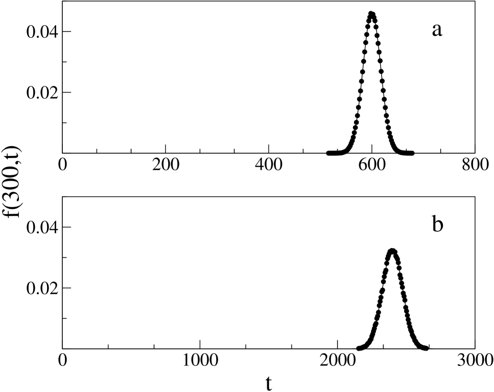
Figure 5: Probability distribution $f(r=300,\,t)$ for propagation in $1-$D and $2-$D lattices. Comparison between numerical simulation results (dots) and theory, Eq.(19) (solid line). (a) $1-$D lattice (see Fig.2a) with $q=0.5$: $c=(3-2\,q)^{-1}=0.5$ and $\gamma=4q(1-q)=1$; half-width $=\sqrt{2\gamma r}=10\sqrt{6}\simeq 24.5$. (b) $2-$D triangular lattice (see Fig.2b) with $q=0.5$: $c=1/8$ and $\gamma=72q(1-q)=18$ (see grosfils ); half-width $=\sqrt{2\gamma r}=60\sqrt{3}\simeq 104$.

The explicit expression (55) for $\tau_{j}$ based on the automaton dynamics yields analytical expressions for $c$ and $\gamma$ in terms of the spin-lattice characteristics and there from in terms of the probability $q$. Concomitantly there is an explicit reference to a feed-back mechanism where the dynamics modifies locally the substrate which in turn modifies the dynamics, and there are systems where this mechanism should be important. However we emphasize that the specification (55) of the delay time $\tau_{j}$ is not indispensable. The propagation-dispersion equation (18) is general as it follows from the continuous limit of the first visit equation (1) without recourse to (55) as shown in Section IV. It suffices that there exists a distribution of time delays with $\sum_{j=0}^{n}\,p_{j}=1$ and with finite moments $\langle\tau^{a}\rangle$, to obtain (18) from (1). This establishes the validity of the propagation-dispersion equation for a class of systems whose dynamics is subject to time-delays independently of the underlying microscopic mechanism responsible for the delays.

References

- (1) See e.g. W. Feller, An Introduction to Probability Theory (Wiley, New York, 3d ed., 1968), Vol.1, section XIV.6.
- (2) I. Ippolito, L. Samson, S. Bourlès, and J.P. Hulin, Eur. Phys. J. E., 3, 227 (2000).
- (3) C.G. Langton, Physica D, 22, 120 (1986); S.E. Troubetskoy, Lewis-Parker Lecture (1997); D. Gale, Tracking the Automatic Ant, Springer (New York, 1998).
- (4) E.G.D. Cohen, “New types of diffusion in lattice gas cellular automata” in Microscopic Simulations of Complex Hydrodynamic Phenomena, M. Mareschal and B. L. Holian, eds., NATO ASI Series B: Physics (1992) Vol. 292, p.145; ; H.F. Meng and E.G.D. Cohen, Phys. Rev. E, 50, 2482 (1994); E.G.D. Cohen and F. Wang, Physica A, 219, 56 (1995).
- (5) P. Grosfils, J.P. Boon, E.G.D. Cohen, and L.A. Bunimovich, J. Stat. Phys., 97, 575 (1999).
- (6) J.P. Boon, J. Stat. Phys., 102, 355 (2001).
- (7) See e.g. N.G. Van Kampen, Stochastic Processes (North-Holland, Amsterdam, 1990), Section VIII-2.
- (8) See e.g. U. Frisch, D. d’Humières, B. Hasslacher, P. Lallemand, Y. Pomeau, and J.P. Rivet, Complex Systems, 1, 649 (1987).
- (9) G.I. Taylor, Proc. London Math. Soc., 120, 196 (1921).
- (10) J. Koplik, in Disorder and Mixing, E. Guyon, J.P. Nadal, and Y. Pomeau, eds. (Kluwer Academic Publishers, Doordrecht, 1988), pp. 123-137.
- (11) C. Pigorsch and G.M. Schütz, J. Phys. A: Math. Gen., 33, 7919 (2000).
- (12) T. Huisinga, R. Barlovic, W. Knospe, A. Schadschneider, and M. Schreckenberg, Physica A, 294, 249 (2001).
- (13) M. Kawasaki, T. Odagaki, and K.W. Kehr, Phys. Rev. B, 61, 5839 (2000).
- (14) D. Chowdhury, L. Santen, and A. Schadschneider, Phys. Reports, 329, 199 (2000).
- (15) R.C. Merton, Continuous-time Finance (Blackwell, Cambridge,1997); J.P. Bouchaud and M. Potters, Theory of Financial Risks: From Statistical Physics to Risk Managements (Cambridge University Press, Cambridge, 2000).
- (16) L.A. Bunimovich and M.A. Khlabystova, J. Stat. Phys., 108, 905 (2002).
- (17) J.P. Boon and P. Grosfils, http://www.arxiv.org, arXiv:cond-mat/0108420.
- (18) L.A. Bunimovich, Physica A, 279, 169 (2000).