Spontaneous structure formation in a network of chaotic units
with variable connection strengths

Abstract

As a model of temporally evolving networks, we consider a globally coupled logistic map with variable connection weights. The model exhibits self-organization of network structure, reflected by the collective behavior of units. Structural order emerges even without any inter-unit synchronization of dynamics. Within this structure, units spontaneously separate into two groups whose distinguishing feature is that the first group possesses many outwardly-directed connections to the second group, while the second group possesses only few outwardly-directed connections to the first. The relevance of the results to structure formation in neural networks is briefly discussed.

Recently, studies of various types of networks have been attracting the interest of researchers from a broad range of scientific diciplines [1, 2]. Although in some such studies, there is a time dependence of the structure of the network consisting of an increase in the number of units of which it is composed [2], the elements themselves are essentially static units, with neither their intrinsic properties nor their interactions with each other evolving in time. Most networks in the real world, however, consist of dynamic elements, and the dynamics of the individual elements influence the formation of network structure. Thus in order to understand realistic networks, it is necessary to consider the modeling of networks with such dynamic elements. In this Letter we study an abstract model of a network composed of dynamic elements and report its behavior, as found through numerical simulation, focusing mainly on the formation of structure.

We consider a network of $N$ dynamic units that interact with each other through connections with time-dependent strengths. For simplicity, we describe the dynamics of both the units and the connection strengths with discrete-time maps. Hence, our model belongs to a class of globally coupled maps (GCM) [3]. We denote by $f(x)$ the function defining the map for the dynamics of each unit. With this, our model is given by the set of equations

$$x^{i}_{n+1}=f[(1-c)x^{i}_{n}+c\sum^{N}_{j=1}w^{ij}_{n}x^{j}_{n}],$$ (1)

where $x^{i}_{n}$ is the state variable of the $i$-th unit ($1\leq i\leq N$) at the $n$-th time step. The coupling $c$ represents the strength of the influence of the other units on the dynamics of unit $i$ ($0<c<1$), and $w^{ij}_{n}$ is the time-dependent weight of the connection from the unit $j$ to $i$ at time step $n$. As the map providing the dynamics of the units, we adopt the logistic map $f(x)=ax(1-x)$, but we believe that qualitatively similar behavior would be displayed by the system for any form of $f(x)$ that exhibits chaos.

With regard to the dynamics of the connection strengths, we stipulate that the connections between units $i$ and $j$ with similar values $x^{i}_{n}$ and $x^{j}_{n}$ are strenghened [4, 6]. (This can be regarded as an extension of Hebb’s rule, which is widely used in neural network studies [5].) Also, we consider there to be a resource in the system that is used to establish connections between units. Then, we assume that there is a limitation on this resource. As a result, there exists competetion among connections for this resource. Instead of using an explicit variable representing the resource, we incorporate this effect into our model through the normalization of the connection strengths, as

$$w^{ij}_{n+1}=\frac{[1+\delta\cdot g(x^{i}_{n},x^{j}_{n})]w^{ij}_{n}}{\sum_{j=1}^{N}[1+\delta\cdot g(x^{i}_{n},x^{j}_{n})]w^{ij}_{n}},$$ (2)

where $\delta$ is a parameter that represents the plasticity of the connection strengths, and $g(x^{i}_{n},x^{j}_{n})$ is a monotonically decreasing function of the absolute value of the difference between its arguments, whose form we choose here is $g(x^{i}_{n},x^{j}_{n})=1-2|x^{i}_{n}-x^{j}_{n}|$. Note that, due to the normalization given in Eq. (2), $w^{ij}$ is generally not equal to $w^{ji}$; i.e., the network is asymmetric.

In the following, we give the results of our numerical simulations of the model. Throughout this Letter, the number of units $N$ is set to $100$, though the results described below do not change qualitatively for larger systems except for the existence of a longer transient behavior. The initial conditions we used are as follows. First, the initial values of the self-connections $w^{ii}_{0}$ were set to $0$. Then as determined by Eq. (2), they remained at $0$ for $n>0$. Second, all the remaining connection strengths were set to identical values. From the constraint of the normalization, this value is determined to be $1/(N-1)$. Finally, for the state variables, the initial values were randomly chosen from the interval $(0,1)$ with a uniform sampling measure.

In our model, we have three parameters: $a$, which controls the dynamics of each unit, $c$, which determines the overall sterngth of the interactions between the units, and $\delta$, which governs the connection dynamics. Here we fix the parameter $\delta$ to $0.1$ [7] and study how the behavior of the system changes as the function of the values of the parameters $a$ and $c$.

It is known that the dynamics of GCM can be classified into four phases, according to the degree of synchronization and clustering among units [3]. In contrast to the conventional GCM, only three of these four phases appear in our system. The first is the coherent phase, in which all the units take the same value and oscillate synchronously. The second is the ordered phase, in which the units split into a few clusters and all the units within each such cluster oscillate synchronously. The third is the desynchronized phase, in which there is no synchronization between any two units [8].

Corresponding to the different types of collective behavior, different network structures emerge. In the coherent phase, all connections have almost identical values and these values do not change over time. In the ordered phase, due to the formation of clusters of units, connections between units that belong to the same cluster have similar finite values, determined by the size of the cluster, while connections between two units from different clusters tend towards $0$. In this case too, the network is static. The situation is different, however, in the desynchronized phase, in which connection strengths can change, and the network structure is not fixed over time. The structure of the network in this phase is complicated, but not completely random. In this Letter we consider only the phenomena observed in this desynchronized phase, because we are presently interested in the behavior of dynamic networks. This phase roughly corresponds to the parameter ranges $3.7<a<4.0$ and $0<c<0.2$. In the simulations reported in th following, parameter values outside these ranges were not used.

To characterize the global behavior of the network in the parameter space, we define some characteristic quantities of the network and study their parameter dependence.

First, as an index of the magnitude of the temporal change of the network, we define an average variation of the connection strength per step. We call this the ‘activity of the network’, and write it

$$A=\frac{1}{(N-1)^{2}}\cdot\frac{1}{\tau_{m}}\sum_{i\neq j}\sum_{n=\tau_{t}}^{\tau_{t}+\tau_{m}}|w_{n}^{ij}-w_{n-1}^{ij}|,$$ (3)

where $\tau_{t}$ is the length of the transient period and $\tau_{m}$ is the length of the measuring period.

In FIG. 1(a), the activity $A$ of the network is plotted with respect to the parameters $a$ and $c$ on a gray scale. Here $\tau_{t}$ and $\tau_{m}$ were chosen as $100,000$ and $1,000$, respectively. A broad band of high activity is seen around the line $c=.15\times(a-3.7)$, corresponding to the bright region in FIG. 1(a). Note that there is no synchronization between the dynamics of the units anywhere in the parameter space shown in Fig 1(a), Nevertheless, there is a rather wide region of quite low activity. In most of this region, most of th units exist in pairs, with the units in each such pair having non-zero connections only between each other, forming fixed pairs in the network. While the dynamics of two units forming a pair are not synchronized, they are highly correlated.

In the regime of high activity, more complex and dynamic network structure is formed. To observe this, we consider the average connection matrix, denoted as $W^{ij}$ and defined as the temporal average of $w_{n}^{ij}$: $W^{ij}=\frac{1}{\tau_{m}}\sum_{n=\tau_{t}}^{\tau_{t}+\tau_{m}}w_{n}^{ij},$ where $\tau_{m}$ and $\tau_{t}$ were introduced in Eq. (3).

If the dynamics of the connection strength are completely random, it is expected that the average connection strengths will take almost identical values for each $i$ and $j$, and the variance among units will decrease to 0 as the averaging time increased. Contrastingly, if there exists structure in a network with high activity, there should be some variance among units in $W^{ij}$. Keeping this in mind, we consider the sum of the average connection strengths eminating from one unit: $W_{out}^{i}=\sum_{j=1}^{N}W^{ji}$. We calculated the variance of $W_{out}^{i}$ over $i$ for different parameter values. The result is displayed in FIG. 1(b) for $\tau_{t}=100,000$ and $\tau_{m}=1,000$. We find that a large variance is observed just below the line $c=.15\times(a-3.7)$.

Comparing FIG.s 1(a) and (b), we can see that the region of high network activity can be decomposed into two regimes: one with a large variance of $W_{out}^{i}$ [for $c<.15\times(a-3.7)$], and the other with small $W_{out}^{i}$ [for $c>.15\times(a-3.7)$]. As mentioned above, a large variance in the active regime indicates the existence of some structural order in a temporally evolving network.

In the following, we investigate the structural characteristics of this dynamic yet ordered network. In particular we consider the parameter values $a=3.97$ and $c=0.12$, which correspond to the largest variance in the active regime However we point out that the general characteristics of the network do not depend sensitively on this special choice of the parameter values.

First, we study the structural change over time from the initial all-to-all type network to the eventual highly structured one, by considering the dependence on the averaging time of $W_{out}^{i}$. In FIG. 2, we plot series of $W_{out}^{i}$ as functions of the measuring time $\tau_{m}$ (with fixed transient time $\tau_{t}=0$) for a single trial [9]. Each line represents a series of $W_{out}^{i}$ for a particular value of $i$.

This figure shows that units separate into two groups: one with large values of $W_{out}^{i}$ and one with small values [10].The separation becomes more distinct as the measuring time increases, although the separation process seems to be nearly completed by the $3\times 10^{6}$-th step, because after this time, we do not observe the migration of any unit between the two groups. Also, this figure shows that the fluctuations of $W_{out}^{i}$ are larger for the large $W_{out}^{i}$ group. This implies that $W_{out}^{i}$ for a unit in this group occasionally takes small values for a certain period. By contrast, a unit of the small $W_{out}^{i}$ group will only very rarely take large values of the total weight. In this sense, the small $W_{out}^{i}$ group is more stable.

To quantify the detailed properties of the network structure, we digitize the connections as follows: If $w^{ij}$ exceeds a threshold value, namely $1/(N-1)$, we assign a connection from unit $j$ to unit $i$; otherwise no connection is assigned. This threshold $1/(N-1)$ is equal to the connection value in the case that a unit uniformly connects to all the others. Hence it is a natural criterion for distinguishing ‘strong’ connections.

Using this method, we can represent the network by a graph. We composed graphs from snapshots of $w^{ij}$ at the $500,000$-th step for many initial conditions. From these graphs, we calculated distribution of the degree of reception and emission. The degree of reception is the number of connections directed at a unit (subsequently reffered to as “inwardly-directed” connections) and the degree of emission is the number of connections eminating from a unit (subsequently reffered to as “outwardly-directed connections”.) The distributions of these two quantities are shown in FIG. 3.

The distribution of the degree of reception has a unimodal shape, with a peak at about $8$ degrees. Hence, with regard to the inwardly-directed connections, this network has a single scale. This is mainly due to the competition among inwardly-directed connections, resulting from their normalization.

By contrast, the distribution of the degree of emission has a bimodal shape, which can be decomposed into two components. One component is a distribution with exponential decay, corresponding to the small $W_{out}^{i}$ group in FIG. 2. The nother component is the unimodal distribution with a peak at about $45$ degrees, corresponding to the large $W_{out}^{i}$ group in FIG. 2.

Considering the appearance of the two components in the distribution of the outwardly-directed connections, we divide the units into two groups. One group we call the ‘core group,’ which consists of units with more than $20$ connections, and the other we call the ‘peripheral group,’ which consists of all other units. With the parameter values used here, the number of units in the core group is typically 14.

With the partition of units into these two groups, the connections are naturally classified into four groups. The group to which a given connection belongs is determined by the groups to which the two units it connects belong. With obvious identification, we call these groups the ‘core-to-core group’, the ‘core-to-peripheral group’, the ’peripheral-to-core group’, and the ‘peripheral-to-peripheral group’.

The number and density of connections in each group are listed in Table 1. The most apparent characteristics seen here are that the peripheral-to-core group has very few members, while the core-to-peripheral group has many members. Also, it is senn that the density of core-to-core connections is quite high and that of peripheral-to-peripheral connection is quite low. From these results, we can conclude that the units in the core group interact strongly with each other and that the dynamics of the core group strongly influence the peripheral group, but that the dynamics of the peripheral group have almost no influence on the core group.

To this point, we have investigated our system mainly with regard to network structure, largely ignoring the dynamics of units underlying the structure formation. However, it is clear that there must be interdependency of the unit dynamics and connection dynamics for the structure formation discussed above to occur. We have confirmed this directly through numerical simulations. Using the somewhat unnatural restriction under which connection weights depend on the dynamics of the units but that the dynamics of the units do not depend on the connection weights, we found that no structure ever appears. More detailed analysis of this point is now underway and its results will be presented elsewhere.

To summarize, as a model of temporally evolving networks, we have considered a network of dynamic units, whose dynamics are described by logistic maps and which are coupled to each other with variable connection weights. The model exhibits dynamical self-organization of its network structure, reflected by the state of units’ collective behavior. Even in the parameter region where there is no synchronization of the unit dynamics, some structural order emerges. There, units spontaneously separate into two groups, with one group possessing especially many outwardly-directed connections to the other group.

Because of the simplicity of the model and the universality among globally coupled maps, we believe that the phenomena revealed in this study are exhibited generally by a network whose connections change in a manner governed by the relationships between its dynamic elements. One example is neural networks. Though the conventional understanding has been that the timescale of the change of synaptic weights is much slower than that of neuronal dynamics, more and more evidence is being published providing evidence that synaptic change occurs over a wide range of timescales, from hundreds of milliseconds to months or years [11]. In addition, it is known that, in the early stage of development, axons arborize excessively, and eventually are trimmed under the influence of neuronal activity [12]. Our model seems to be suited to the modeling of such a situation. The structure formation observed in this study may provide a basic description of local structure formation in the brain, such as columnar structure.

As mentioned at the beginning of this Letter, there is yet little known about dynamic networks. The significance of our study will be revealed as empirical data about dynamic networks are obtained.

The authors would like to thank T. Ohira for his valuable suggestions, and to G. C. Paquette for the critical reading of the manuscript. This work is supported by Grants-in-Aid for Scientific Research from Ministry of Education, Science and Culture of Japan (11CE2006).

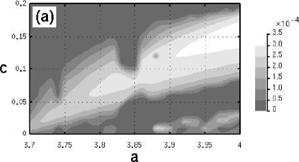
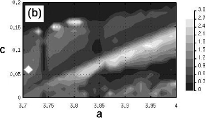
FIG. 1.: Gray scale plots of network quantities with respect to the parameters $a$ and $c$, with a discretization of 0.01 for both. (a) The activity $A$ of the network. Brighter color corresponds to higher network activity. (See the text for the definition of the quantity $A$.) (b) The variance of the total weight of outwardly-directed connections $W_{out}^{i}$. Brighter color corresponds to larger variance.

FIG. 2.: The total weights of outwardly-directed connections $W_{out}^{i}$ as functions of the measuring time for the average connection matrix $W^{ij}$. Each curve corresponds to a single unit and represents a series of $W_{out}^{i}$ with different measuring times. The series of $W_{out}^{i}$ for all units are superimposed.

FIG. 3.: Distributions of the degrees of reception and emission. A logarithmic scale is used for the vertical axis. The solid curve is the distribution of the degree of emission, and the broken line is that of the degree of reception.

Group	No. of connections	density
CC	159	0.6625
CP	792	0.5893
PC	2	0.0015
PP	234	0.0336

TABLE I.: Number and density of connections in each group. Here, CC, CP, PC and PP denote the core-to-core, core-to-peripheral, perhipheral-to-core and peripheral-to-peripheral groups. (See the text for the definitions of the groups.)

REFERENCES

- [1] D.J. Watts and S. H. Strogatz, Nature 393, 440 (1998).
- [2] A. -L. Barabasi and R. Albert, Science 286, 509 (1999).
- [3] K. Kaneko, Physica 41D, 137, (1990); 54D, 5, (1991).
- [4] K. Kaneko, Physica 75D, 55, (1994).
- [5] J. A. Hertz, A. Krogh and R. G. Palmer, Introduction to the Theory of Neural Computation (Addison-Wesley, Redwood City, 1991).
- [6] J. Ito and K. Kaneko, Neural Networks 13, 275, (2000).
- [7] Qualitatively similar behavior is observed over a wide range of values of , but for very small values, (say ,) we have not observed the network structure discussed here. The timescales of the unit dynamics and connection dynamics must be set to be of the same order.
- [8] The phase with many synchronized clusters (partially ordered phase) observed in conventional GCM does not exist here. This is due to the randomness of the connections in the present model. [See S. C. Manrubia and A. S. Mikhailov, Phys. Rev. E 60, 1579, (1999).]
- [9] Here we have not plotted the timeseries of themselves, as we wish to illustrate the separation of the units clearly.
- [10] In FIG. 2, the separation is amplified due to longer averaging times for larger . However, we have confirmed from a direct plot of that after transient behavior dies out, if a given ever takes a sufficiently small value, it never again joins the large group, and if it ever takes a sufficiently large value, it never again joins to the small group. Also, it should e noted that the fluctuations of the in the upper group are larger than those in the lower group, but even with ther large fluctuations, these do not fall to the level of the small group.
- [11] W. Maass and A. M. Zador, in Pulsed Neural Networks, edited by W. Maass and C. M. Bishop (MIT Press, Cambridge, 2001).
- [12] D. Purves and J.W. Lichtman, Science 210, 153, (1980).