Friction law for dense granular flows: application to the motion of a mass down a rough inclined plane.

Abstract

The problem of the spreading of a granular mass released at the top of a rough inclined plane was investigated. We experimentally measure the evolution of the avalanche from the initiation up to the deposit using a Moir image processing technique. The results are quantitatively compared with the prediction of an hydrodynamic model based on depth averaged equations. In the model, the interaction between the flowing layer and the rough bottom is described by a non trivial friction force whose expression is derived from measurements on steady uniform flows. We show that the spreading of the mass is quantitatively predicted by the model when the mass is released on a plane free of particles. When an avalanche is triggered on an initially static layer, the model fails in quantitatively predicting the propagation but qualitatively captures the evolution.

1 Introduction

Gravity driven geophysical events sometimes involve the flow of a dry granular material. Landslides, rock avalanches and pyroclastic flows are examples of natural hazards where a granular mass flows down a slope. One of the main issues is to predict the flow trajectory over the complex topography, the velocity and the runout distance in order to define a safety zone.

The difficulty in describing granular geophysical flows lies in the uncertainty in the constitutive equations for the flow of dry granular media. Constitutive equations are known for rapid granular flows in a low concentration regime, when the particles interactions are dominated by the collisions . For this regime, a kinetic theory can be developed based on the kinetic theory of dense gases taking into account the dissipation during the collisions ([Haff 1983, Lun et al 1984, Azanza et al 1999, Goldhirsch 1999]). However, for dense flows when the particles not only undergo collisions but also friction and multicontact interactions with neighboring particles, the kinetic approach is no longer valid. Some attempts have been made to incorporate into the kinetic theory which describes the collisional interactions, an empirical rate independent stress tensor in order to take into account the friction ([Savage 1983, Johnson et al 1990, Anderson & Jackson 1992]). However, it is not clear that these approaches are valid for dense flows when multi particles contacts are present. More recently, Savage (1998) proposed an analysis for high concentration flows based on a fluctuating plasticity model which has not yet been applied for flow down slopes. Another approach has been suggested by Mills et al (1999,2000) which is based on the idea that force chains are present in the media inducing a non local formulation of the stresses.

A promising approach for describing unsteady and non uniform flow on complex geometry such as geophysical flows, is the depth averaged St Venant (1871) approach . In this framework, the material is assumed to be incompressible and the mass and momentum equations are written in a depth averaged form. This analysis is valid under the assumption that the flowing layer is thin compared to its lateral extension which is often the case for geophysical flows. Depth averaging allows to avoid a complete 3D description of the flow: the complex rheology of the granular material is incorporated in a single term describing the frictional stress that develops at the interface between the flowing material and the rough surface. Our goal in this paper is to propose an expression for this friction force based on experimental measurements, and to quantitatively compare the prediction of the depth averaged approach with well controlled experiments of granular avalanches.

Depth averaged equations have been introduced in the context of granular flows by Savage and Hutter (1989). In their model, the interaction between the granular material and the rough surface is described by a simple friction law: the shear stress at the bottom is proportional to the normal stress, the coefficient of friction being a constant. The model works well when the surface of the plane is smooth enough: Savage, Hutter and coworkers were able to predicts the motion and spreading of a granular mass on steep slopes in two and three dimensions ([Savage & Hutter 1989, Wielandet al 1999, Gray et al 1999]) . Experiments have been also carried out on curved beds ([Greve & Hutter 1993, Greve et al 1994, Koch et al 1994]), and the measurements agree relatively well with the prediction of the depth averaged model. However, all the experiments have been carried out with high inclinations (higher than $40^{o}$) and with relatively smooth beds (typically 3mm beads rolling on flat surfaces or sand paper).

For the flow of granular material on rough surfaces (where the roughness of the bed is of the order of the particle size) and for moderate inclinations, the description in term of a simple solid friction no longer holds. This is shown by several experimental observations:

a) First, it has been shown that steady uniform flows are observed in a range of inclination angles ([Suzuki & Tanaka 1971, Hungr & Morgenstern 1984, Vallance 1994, Ancey et al 1996, Pouliquen 1999a]). This implies that the bed shear stress is not a simple solid friction but has a velocity dependence in order to balance the gravity for different inclinations.

b) Secondly, the onset of flow on rough inclined planes is not precisely described by the simple solid friction law. According to this law, the flow is possible as soon as the inclination is higher than the friction angle. Experiments reveal a more complex behavior: the onset of flow depends both on the inclination of the plane and on the thickness of the granular layer ([Pouliquen & Renaut 1996, Daerr & Douady 1999, Pouliquen 1999a]). A thin layer has more difficulty to flow than a thick one.

c) Thirdly, an hysteresis is observed between flowing and static states. A static layer of material resting on a rough surface will start flowing at a given threshold of the inclination. However it will not stop before the slope decreases below a second threshold. In between these two angles there exist metastable states, where avalanches can be triggered by perturbations. The complex and rich dynamics of the avalanches has been recently studied by Daerr and Douady (1999) and Daerr (2001).

All these features can not be captured by the simple solid friction assumption. The question we want to address in this study is the following: can we find a more realistic friction law within the depth averaged framework which can capture the behavior of thin granular layers on rough planes? In a previous work ([Pouliquen 1999a]), we have proposed an empirical friction law based on scaling properties measured for steady uniform flows. We have shown that a depth averaged description taking into account this friction predicts the steady shape of granular fronts propagating down a slope ([Pouliquen 1999b]). However, unsteady flows where static material start to move, or moving material comes to rest, involve a complex dynamics which is not a priori taking into account in the friction law. In the present study our goal is to check to what extent the empirical friction law found for steady uniform flows can be used in the framework of the depth averaged equations to quantitatively predict unsteady and non uniform flows where deposit are formed and avalanches are triggered.

To this end, we have investigated two different experimental configurations. The first one is the spreading of a granular mass released at the top of a rough inclined plane. The second is the release of a mass on a static layer of grains initially present on the rough plane. With the first configuration we can study how the material comes to rest and creates a deposit, whereas with the second we can study how static material is put into motion by flowing material. In both configurations the time evolution of the mass is measured and compared with the predictions of the depth averaged model.

The experimental setup and the measurement procedure are presented in Section 2. In Section 3 the depth averaged model is described and the choice of the friction law is discussed. The results are presented in Section 4. Discussion about the sensitivity of the model to the parameters is given in Section 5 before concluding about the relevance and limits of the depth averaged approach in Section 6.

2 Experimental configurations

2.1 Experimental setup

The experimental setup is a 2m long and 70cm wide rough plane whose inclination $\theta$ can be precisely controlled. The surface is made rough by gluing one layer of particles on the plane. The particles we used are glass beads 0.5mm $\pm 0.04$ in diameter. The first set of experiments consists in removing a spherical cap full of beads at the top of the plane. The released material then starts flowing down the slope, the mass spreads and ultimately stops leaving a tear shaped deposit (Fig. 1a). Three roughly homothetic spherical caps have been used: a small one ($r=2.1$ cm $R=3.7$ cm), a medium one ($r=3.1$ cm $R=6$ cm) and a large one ($r=4$ cm $R=8$ cm, see Fig. 1a for the definition of $r$ and $R$ ). In order to precisely control the amount of material present in the cap, the mass of beads poured in the cap is initially weighed before each run (62 g for the small cap, 231 g for the medium one, 524 g for the large cap).

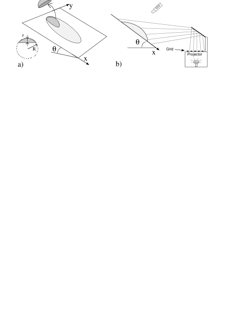
Figure 1: a) Sketch of the experimental set-up. The spherical caps we used are part of a sphere of radius R. b) Visualisation method.

In a second set of experiments the mass is released on the top of a layer of material already lying on the surface. The initially static layer is prepared by creating a steady uniform flow over the whole surface and by suddenly stopping the supply. In this case, a uniform deposit is created with a well defined thickness $h_{stop}$ depending only on the inclination $\theta$ ([Pouliquen 1999a]). The spherical cap is then carefully placed on the layer and filled with the beads. When the cap is suddenly removed, the mass spreads out putting into motion some of the initially static material, triggering an avalanching front.

2.2 Measurement method

In order to measure precisely the time evolution of the granular mass, we have developed a method inspired by a Moiré method ([Sansoni et al 1999]). A grid pattern made of horizontal lines is projected on the plane by an overhead projector as sketched in Fig. 1b. The projection angle is small enough such that the presence of the granular mass on the surface induces a significant deformation of the grid (Fig. 2b). Pictures of the plane are recorded by a CCD camera positioned at the vertical of the plane. The local shift of the lines observed between the deformed pattern in the presence of a granular mass (Fig.2b) and the initial regular pattern when the surface is flat (Fig.2a) is proportional to the local thickness of the granular layer. In order to quantitatively get the thickness $h(x,y)$ we proceed as follows. The reference picture Fig. 2a and the picture to be analyzed Fig. 2b are digitalized which gives two real amplitudes $A_{ref}(x,y)$ and $A(x,y)$. The 2D spatial Fourier transforms of both amplitudes are then computed. Both pictures being close to a regular pattern, the Fourier transforms are found to present well defined peaks at the complex wavenumbers $(2\pi/\lambda,0)$ and $(-2\pi/\lambda,0)$, $\lambda$ being the wavelength of the projected grid. For Fig. 2b, the information about the slight deviation from the reference pattern induced by the granular mass is contained in the width of the peak. In order to extract the phase of the picture, the right half of the wavenumber spectrum ($k_{x}>0$) is used to reconstruct two complex amplitudes $A^{c}_{ref}(x,y)$ and $A^{c}(x,y)$. The phase $\phi_{ref}(x,y)$ and $\phi(x,y)$ of $A^{c}_{ref}$ and $A^{c}$ gives the phase of the pattern in picture 2a and 2b. The thickness $h(x,y)$ is then simply proportional to the phase difference $\phi(x,y)-\phi_{ref}(x,y)$. The coefficient of proportionality is found by measuring the phase shift induced by a 1cm thick plate. The Figure 2c shows the contours of constant thickness given by the analysis.

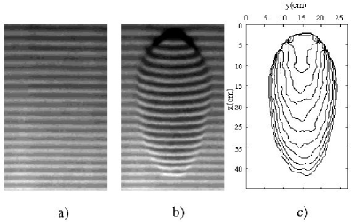
Figure 2: a) Reference picture; b) Picture to be analyzed; c) Contours of constant thickness every 0.5mm given by the phase difference between picture a) and b).

The time evolution of the free surface of the mass $h(x,y,t)$ is obtained by analyzing by this method each image of a movie recorded during the flow. The thickness measurement is estimated to be precise up to $\pm 0.3$mm. The phase measurement method breaks down when shadows are present behind the mass as in Fig 2b. In the region close to the shadow, the thickness is not correctly estimated and the contour of the deposit is not correct. The contour in this region is then estimated from direct visualisation of the pictures. However, shadows are observed only at the first stage of the spreading when the layer is thick.

3 Theoretical model

3.1 Depth averaged equations

The use of depth averaged equations to describe the flows under consideration here is motivated by the large aspect ratio of the granular mass: its lateral extension is large compare to the thickness of the layer.

More precisely, in order to derive the St Venant equations we assume that the variation of the flow takes place on lengths much larger than the thickness. Assuming in addition that the flow is incompressible of constant density $\rho$, which is justified for the dense flow regim studied here [Savage & Hutter 1989, Ertas et al 2001], we obtain the depth averaged mass and momentum conservations by integrating the full 3D equations ([Savage & Hutter 1989]). The following equations are written in terms of the local thickness $h(x,y,t)$ and the depth averaged velocity ${\bf u}(x,y,t)=u{\bf e}_{x}+v{\bf e}_{y}$:

$$\displaystyle\frac{\partial h}{\partial t}+\displaystyle\frac{\partial(hu)}{\partial x}+\displaystyle\frac{\partial(hv)}{\partial y} = 0,$$ (1)

$$\rho\left(\displaystyle\frac{\partial(h{\bf u})}{\partial t}+\alpha{\bf\nabla}\cdot\left(h{\bf u}\otimes{\bf u}\right)\right) = \rho gh\cos\theta\left(\tan\theta{\bf e}_{x}-\mu\left(h,\|{\bf u}\|\right)\displaystyle\frac{{\bf u}}{\|{\bf u}\|}-K{\bf\nabla}h\right),$$ (2)

Equation 1 is the mass conservation. Equation 2 is the momentum conservation where the acceleration is balanced by three forces. In the acceleration expression, the coefficient $\alpha$ is related to the assumed velocity profile across the layer. In the case of a plug flow, $\alpha=1$ whereas for a linear profile $\alpha=4/3$. For sake of simplicity we will used in the following $\alpha=1$, the results being not sensitive to the choice of $\alpha$ as we will discuss in section 5. The first force on the right-hand side is the gravity parallel to the plane which is the driving force. The second term is the shear stress at the base: it is opposed to the motion, and is written as a friction coefficient $\mu$ times the vertical normal stress $\rho gh\cos\theta$. The friction coefficient a priori depends on the local thickness $h$ and the local velocity $\|{\bf u}\|$. The last term in eq. 2 represents the pressure force linked to the thickness gradient. The coefficient $K$ represents the ratio of the vertical normal stress to the horizontal one ([Savage & Hutter 1989]). For quasi-static deformation this coefficient can be calculated from standard Mohr-Coulomb plasticity model as done by Savage and Hutter (1989). However, for dense granular flows on rough surfaces the material behaves more like a fluid. Numerical simulations tend to show that the vertical and horizontal normal stresses are equal ([Prochnow et al 2000, Ertas et al 2001]). We then choose in the rest of the paper $K=1$. This choice will be discussed in Section 5.

In order to apply those equations to describe granular flows, one has to give the expression for the friction law $\mu\left(h,\|{\bf u}\|\right)$. No theory exists for determining the bottom shear stress in the dense regime. A first approximation is to consider the friction coefficient as constant. This approximation works well when the surface is smooth but does not predict correct results for flows on surface whose roughness is of the order of the particle diameter. Here we use a more complex friction law based on previous experimental results obtained for steady uniform flows.

3.2 The empirical friction law

First, information about the friction mobilized in thin granular layer is given by the onset of the flow. Experimental measurements have shown the existence of two critical angles: an initially static granular layer starts to flow when the inclination reaches a critical value $\theta_{start}$. To stop the flow, one has to decrease the inclination down to a lower angle $\theta_{stop}$. The important result for the case of a layer on rough inclines is that the two angles are function of the initial thickness $h$ of the layer as shown in Fig.3 for the case of the glass beads used in our experiments. The two curves $\theta_{stop}(h)$ and $\theta_{start}(h)$ have the same shape but are translated one from another by roughly one degree. The same behavior is observed with different materials on different roughness conditions ([Pouliquen & Renaut 1996, Daerr & Douady 1999]). In the following we defined the tangent of these angles $\mu_{start}(h)=\tan\left(\theta_{start}(h)\right)$ and $\mu_{stop}(h)=\tan\left(\theta_{stop}(h)\right)$. We show below that the knowledge of these two functions is sufficient to define the empirical friction law $\mu\left(h,\|{\bf u}\|\right)$ in the whole range of velocity and thickness.

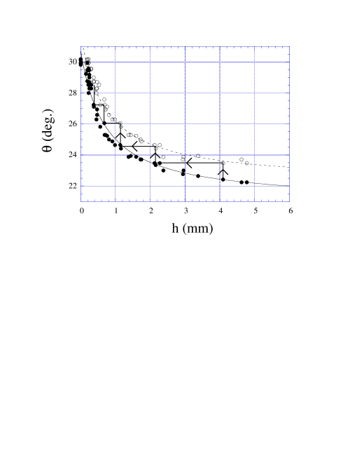
Figure 3: Variation of the starting ($\circ$) and stopping ($\bullet$) angles as a function of the thickness $h$. The arrows indicate the way they are measured: starting with a uniform layer $h$, $\theta$ is increased up to the point where an avalanche occurs. After the avalanche, $h$ has a lower value, $\theta$ is increased again and so on. In the $(h,\theta)$ plane one oscillates between the starting and stopping curves.

We have shown in a previous paper ([Pouliquen 1999a]) that the friction coefficient $\mu\left(h,\|{\bf u}\|\right)$ is related to the function $\mu_{stop}(h)$ by the relation

$$\mu\left(h,\|{\bf u}\|\right)=\mu_{stop}\left(h\frac{\beta\sqrt{gh}}{\|{\bf u}\|}\right)$$ (3)

where $\beta$ is a constant equal to 0.136 for glass beads, independent of the roughness conditions.

This non trivial result comes from properties observed for steady uniform flows ([Pouliquen 1999a]). Steady uniform flows are controlled by the balance between friction and gravity which according to eq.2 gives $\mu(h,\|{\bf u}\|)=\tan\theta$. To find the function $\mu$ one simply has to know how the mean velocity $\|{\bf u}\|$ varies with the two control parameters $h$ and $\theta$. Taking the inverse of the relation $\|{\bf u}\|(h,\theta)$ gives $\mu(h,\|{\bf u}\|)$. Our measurements have shown that the mean velocity $\|{\bf u}\|$, the thickness of the granular layer $h$, and the inclination angle $\theta$ are related through the following relation:

$$\frac{\|{\bf u}\|}{\sqrt{gh}}=\beta\frac{h}{h_{stop}(\theta)}.$$ (4)

The function $h_{stop}(\theta)$ is the thickness of the deposit left by a steady uniform flow at the inclination $\theta$. It is simply the inverse function of $\theta_{stop}(h)$. The expression of the friction coefficient eq. 3 is then obtained by substituting $\theta$ by $\tan^{-1}(\mu)$ in the velocity expression eq.4.

However, the scaling law 4 is only valid for a Froude number defined as $Fr=\|{\bf u}\|/\sqrt{gh}$ greater than $\beta$: no steady uniform flow is observed with a lower Froude number, i.e. with a thickness $h$ less than $h_{stop}$. It follows that the friction law 3 is only valid for $Fr>\beta$.

For $Fr<\beta$ we have no information about the friction law. Experiments on friction between solids ([Heslot et al 1994]) or between a rough plate and a granular layer ([Nasuno et al 1997]) in the low velocity regime have shown a complex and rich dynamics not yet fully understood. As a first approximation, the important point is that the friction coefficient first decreases when increasing the velocity down to a minimum where it starts to increase. The velocity declining part is a source of instabilities ([Heslot et al 1994, Baumberger et al 1994]). The fact that no steady uniform flow is observed for $Fr<\beta$ in our granular system suggests that the friction coefficient in this range decreases when increasing the Froude number. For $Fr<\beta$ we then assume that the friction coefficient $\mu\left(h,\|{\bf u}\|\right)$ tends to the static friction coefficient $\mu_{start}(h)$ when velocity goes to zero. In between $Fr=0$ and $Fr=\beta$, we simply extrapolate by a power function characterized by a power $\gamma$.

The final expression for the friction coefficient can then be written as follows (in terms of the thickness $h$ and the local Froude number $Fr=\|{\bf u}\|/\sqrt{gh}$ instead of $h$ and $\|{\bf u}\|$ ):

If $Fr>\beta$:

$$\mu(h,Fr)=\mu_{stop}\left(h\frac{\beta}{Fr}\right)$$ (5)

if $0<Fr<\beta$:

$$\mu(h,Fr)=\left(\displaystyle\frac{Fr}{\beta}\right)^{\gamma}\left(\mu_{stopstart}(h)-\mu_{start}(h)\right)+\mu_{start}(h)$$ (6)

if $Fr=0$:

$$\mu(h,0)=min\left(\mu_{start}(h),\|\tan\theta{\bf e}_{x}-K{\bf\nabla}.h\|\right).$$ (7)

The last expression is just to ensure that, when the material is static, the friction exactly balances the other forces unless the total force reaches the threshold value given by the static friction coefficient.

The crucial point is that the above friction force is quantitatively determined by the two functions $\mu_{stop}(h)$ and $\mu_{start}(h)$ that can be easily measured in the experiments. For the glass beads used in the experiments the best fits (Fig. 3) are given by:

$$\mu_{stop}(h)=\tan\delta_{1}+\left(\tan\delta_{2}-\tan\delta_{1}\right)\displaystyle\frac{1}{h/L+1}$$ (8)

$$\mu_{start}(h)=\tan\delta_{3}+\left(\tan\delta_{2}-\tan\delta_{1}\right)\displaystyle\frac{1}{h/L+1}$$ (9)

with $\delta_{1}=21^{o}$, $\delta_{2}=30.7^{o}$, $\delta_{3}=22.2^{o}$, and $L=0.65$mm.

The only unknown coefficient in the friction law is the power $\gamma$ of the extrapolation at low Froude numbers. We have checked that the prediction of the model are not sensitive to its value as long as $\gamma$ is less than $10^{-2}$. In the simulation $\gamma$ is chosen equal to $10^{-3}$. The sensitivity to the value $\gamma$ will be discussed in Section 5. The friction coefficient $\mu(h,Fr)$ given by equation 3.5-3.9 is plotted in Fig. 4 as a function of the Froude number for different thicknesses. The reader has to keep in mind that only the part in between $Fr=0$ and $Fr=\beta$ is arbitrarily chosen. The value at $Fr=0$ (stars) and for $Fr>\beta$ is quantitatively given by the measurement of the function $\mu_{start}(h)$ and $\mu_{stop}(h)$. The discontinuity in the slope for $Fr=\beta$ is not physical and comes from the simple extrapolation we have chosen for the friction coefficient at low Froude number. We have checked that a smoother extrapolation around $Fr=\beta$ gives the same predictions.

The choice of the friction coefficient described above is such that it predicts the correct velocity for steady uniform flows, and the correct hysteresis for uniform layers (starting and stopping angles). The question is whereas this friction law is sufficient to predict quantitatively more complex avalanching situations when it is introduced in the depth averaged equations 2.

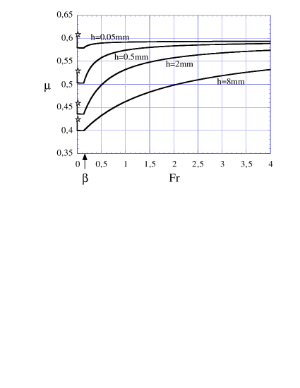
Figure 4: Friction coefficient $\mu(h,Fr)$ as a function of the Froude number $\|u\|/sqrt{gh}$ for different thickness $h$. The stars gives the values for $Fr=0$.

3.3 Numerical methods

In order to numerically solve the depth averaged equations we have used two methods depending on the configuration of interest. For the spreading of the mass on the empty plane, a lagrangian method has been chosen as it allows to easily treat parts where the thickness is zero. The method consists in discretizing the medium in elements which move and deform along with the flow. For the release of the mass on an initially static granular layer where shocks are likely to develop, we have written a shock capturing code based on a first order Godunov scheme. Both numerical schemes are described in detail in the appendix.

4 Results

4.1 Release of a mass on a rough surface.

We first have studied the spreading of the mass on the rough surface free of particles. We have systematically measured the time evolution of the shape of the mass $h(x,y,t)$ for different inclinations and initial volumes and compared with the predicted evolution given by the simulation of the depth averaged equations. No fit parameter exists in the simulation as soon as the functions $\mu_{stop}(h)$ and $\mu_{start}(h)$ are determined.

The time evolution of the spreading for the medium cap at $\theta=23^{o}$ is presented in Fig. 5. The first row of figures shows contours of constant thickness measured in the experiments at five different times. When the material starts to flow the mass rapidly spreads in both directions before it slowly stretches in the slope direction. The rear part of the mass stops (around t=2s), whereas the front forms a bump which propagates down the slope. The mass ultimately stops in a tear like shape. This scenario is well predicted by the theory as shown by the second row of figures in Fig.5 giving the numerical predictions at the corresponding times. The last series of figures is a comparison of the thickness profiles along the longitudinal symmetry axis $y=0$. Satisfactory agreement is obtained between theory and experiments from the initiation of the flow, up to the deposit. The presence of a thicker part flowing at the front when the rear part has already stops (t=2.4s) is well reproduced by the theory.

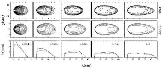
Figure 5: Time evolution of the granular mass for the medium cap $\theta=23^{o}$. First row: experiments. Second row: simulations; Contour of constant thickness every 0.5mm. Third row: thickness profiles along $y=0$; solid line: experiments; dotted line: simulation. The bold circle on the first plot of the simulation represents the initial position of the cap.

The agreement remains correct for different inclinations as shown in Fig. 6 showing the deposits measured in the experiments and predicted by the simulations for different inclination angles. Although the shape of the deposit looks similar from one inclination to another, we have not been able to put in evidence any similarity shape solutions.

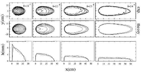
Figure 6: Comparison between experiments (first row) and simulations (second row) for the deposit obtained at different inclinations with the medium cap. Contours of constant thickness every 0.5mm.

The effect of the initial mass has also been studied and the results are presented in Fig. 7. We have plotted the maximum width $W$ and length $L$ of the deposit for the three caps we used, as a function of the inclination. The lines correspond to the prediction of the model, the markers to the experimental observations. The agreement is good for the runout $L$ of the deposit, whereas the lateral spreading $W$ is overestimated by approximately 20%.

It is interesting to compare the above results with the prediction of the simple model using a constant friction coefficient ([Savage & Hutter 1989]). In this case, no deposit is predicted as soon as the inclination of the plane is higher than the friction angle. The whole material flows down the plane. For inclination lower than the friction angle, the pile spreads and stops when its free surface makes an angle with the horizontal equal to the friction angle. In any case, it is not possible with a constant friction law to predict a deposit whose free surface is parallel to the plane as observed in the experiments.

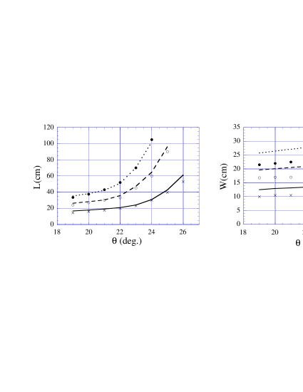
Figure 7: Comparison between experiments (markers) and simulation (lines) for the maximum length $L$ and width $W$ of the deposit as a function of $\theta$ and for three different caps; dotted lines and black circles: large cap; broken lines and white circles: medium cap; Solid lines and crosses: small cap.

4.2 Release of a mass on an initially static layer of material.

The second set of experiments consists in releasing the mass on a static layer of granular material. We first prepare the layer by creating a steady uniform flow at an angle $\theta$ and by suddenly stopping the supply. A uniform deposit of thickness $h_{init}=h_{stop}(\theta)$ lies on the bed. We then carefully put the spherical cap on the layer and filled it with the beads. The mass is then released at t=0s. Result are presented in Fig. 8 for $\theta=23^{o}$ and for the small cap. The first row corresponds to the experimental measurements of the free surface represented by contours of constant thickness. The second row are the corresponding predictions of the simulation. The third row of figures gives the thickness profiles along the longitudinal symmetry axis y=0.

The mass when released rapidly spreads in both directions up to a point when it reaches a drop shape which propagates down the slope without significant deformations. This drop is a wave which put into motion static material at the front and leave static material at the rear. The front is very sharp and the thickness profile along $y=0$ in the stationary regime is triangular as observed previously by Daerr (2001). This wave propagates faster than the material front in the previous deposit experiments described in section 4.1.

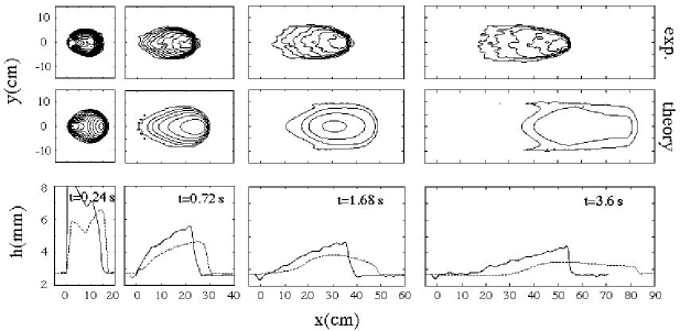
Figure 8: Time evolution of the granular mass released from the small cap on an initial layer of thickness $h_{init}=2.7mm$, $\theta=23^{o}$. First row: experiments. Second row: simulations; Contour of constant thickness every 0.3mm (the external contour line is h=3mm). Third row: thickness profiles along $y=0$; solid line: experiments; dotted line: simulations.

The simulation qualitatively predicts the same dynamics. The mass first spreads in both direction before reaching a roughly constant shape after about 4s (not shown in Fig. 8) which propagates down the slope as a wave. In front of the wave and behind it the material is at rest. Whereas the rapid initial spreading (t¡0.72s) seems to be quantitatively correctly predicted by the model, the long time evolution is no longer in agreement with the experiments. The model predicts a saturated thickness at the front thinner than the one observed in the experiment and the predicted propagation velocity is higher than the one observed. The front of the wave observed in the experiment is also more shocked than the one predicted by the simulations. We have carried out experiments at different inclinations and with the other caps, which reveal the same discrepancy: the depth averaged model predicts always a propagating wave too rapid and too thin compared to the one observed in the experiments.

5 Sensitivity of the model to the parameters

From the two configurations we have investigated we can conclude that the depth averaged model quantitatively predicts the formation of deposit on the plane when the surface is free of particles but fails in predicting the correct avalanche propagation when a static layer is present. In order to better understand the limits of the depth averaged approach we have studied the sensitivity of the simulation to the different parameters introduced in the model. We will then discuss the role of the parameters we have not measured: $\alpha$ in the acceleration term, $K$ in the pressure term, $\gamma$ the power of the extrapolation at low Froude number.

5.1 Role of $\alpha$

The parameter $\alpha$ in the acceleration term in Eq. 2 is obtained when integrating the 3D conservation equations to derive the depth averaged equation. It depends on the assumed velocity profile across the layer. In the simulation presented above $\alpha$ was taken equal to 1 corresponding to a plug flow. For a linear profile $\alpha$ should be taken equal to 4/3. For granular flow on rough inclined plane, previous results suggest that the profile is closer to a linear one than to a plug flow ([Prochnow et al 2000, Ertas et al 2001]). However, the results of the simulation are not very sensitive to the value of $\alpha$. For example, simulations with $\alpha=4/3$ and $\alpha=1$ for the case of Fig. 8 gives a spatio-temporal evolution which differs only by a factor 2% for the thickness and velocities. The reason why the model is so insensitive can be understood by comparing the relative magnitude of the forces acting on the material. Except at the first instants of the spreading, the acceleration is negligible and the friction force balances the gravity forces. In other term, inertia is negligible in the flow regime investigated in our experiments. This can be quantitatively estimated by locally measuring the ratio between the acceleration and the friction force defined by the dimensionless number $R_{f}$:

$$R_{f}(x,y,t)=\frac{\|\tan\theta{\bf e}_{x}-\mu\left(h,\|{\bf u}\|\right)\displaystyle\frac{{\bf u}}{\|{\bf u}\|}-K{\bf\nabla}.h\|}{\mu\left(h,\|{\bf u}\|\right)}.$$ (10)

.

In the case of the deposit experiment of Fig. 5, $R_{f}$ is maximum during the initial rapid spreading where it reaches the value 0.4 (t¡0.5s) and rapidly decreases up to 0.02 everywhere for t¿0.8s. In the case of the flow on a static layer (Fig. 8), $R_{f}$ is less than 0.02 everywhere during the avalanche except at the front where material is put into motion. In this region $R_{f}$ reaches a higher value around 0.1 . We can then conclude that inertial effects are negligible for the dense granular flow we are studying. The choice of $\alpha$ has then no significant influences on the prediction of the depth averaged model for the configuration of interest in this study.

5.2 Role of the pressure coefficient $K$

A second parameter of the model is the pressure coefficient $K$ in front of the thickness gradient term of Eq. 2. This coefficient represents the ratio of the horizontal normal stress to the vertical one. In the results presented above we have used $K=1$ corresponding to an isotropic pressure. This choice has been motivated by several numerical results showing a small difference between the two normal stresses ([Prochnow et al 2000, Ertas et al 2001]). Moreover, we observe that $K=1$ gives the best agreement for the predicted deposits in section 4.1. An example of the prediction with another value of $K$ is shown in Fig 9. We have used the value $K=\frac{1+\sin^{2}\delta_{1}}{1-\sin^{2}\delta_{1}}$ corresponding to the Mohr Coulomb prediction when the basal friction is equal to the internal friction coefficient taken equal to $\tan\delta_{1}$ ([Savage & Hutter 1989]). For our glass beads we obtained $K=1.29$. Using this value, the predicted deposit is wider and shorter than the one experimentally observed. For the case of the flow on the static layer of Fig. 8 the higher value of $K$ predicts also a larger spreading and does not influence the front propagation. Changing $K$ does not provide better agreement for the propagation of the wave.

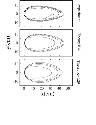
Figure 9: Deposits of the granular mass released from the medium cap $\theta=23^{o}$. a) Experiment; b) Simulation with $K=1$; c) Simulation with $K=1.29$, the value given by the Mohr-Coulomb plasticity criterium.

5.3 Role of the power extrapolation $\gamma$.

The expression of the friction force in our model is quantitatively determined by the two functions $\mu_{stop}(h)$ and $\mu_{start}(h)$ except for the extrapolation at low Froude number. The extrapolation we have chosen is characterized by a power function with an exponent $\gamma$. In the simulation presented above, we have used $\gamma=10^{-3}$. This low value insures a rapid increase of the friction coefficient close to $Fr=0$ (Fig. 4). No influence of $\gamma$ is observed up to $10^{-2}$. If one chooses a larger power ($\gamma>10^{-2}$), the depth averaged model slightly underestimates the runout distance and overestimates the thickness of the deposit, especially at the rear where a small bump is predicted which is not observed. However, the effects are small. For example, for $\theta=23^{o}$ the case $\gamma=1$ predicts a runout distance $L=41cm$ and a maximum deposit thickness of $h=3.3mm$ whereas with $\gamma=10^{-3}$ one get $L=45cm$ and $h=2.8mm$.

For the case of the flow on a static layer, changing the value of $\gamma$ does not significantly changes the front velocity in the Fig. 8.

In conclusion it seems that the discrepancy observed in Fig. 8 between the model and the measurement for the case of the kinematic wave moving on a static layer can not be erased by tuning some of the parameters of the model.

6 Discussion and conclusion

We have shown in this paper that the flow of granular material along rough surfaces can be correctly described by introducing a relevant friction law in a depth averaged description. The spreading of a mass on a rough slope free of particles is quantitatively predicted by the model from the release up to the deposit. The interesting point is that the friction law introduced in the model for describing the interaction between the flowing granular layer and the rough surface is mainly quantitatively determined by the dependence of the stopping and starting angle with the thickness of the layer. Measuring these angles is enough to predict the velocity, the shape and the run-out of the mass.

However, we have shown in this study that the agreement is no longer correct when studying the release of the mass on a uniform granular layer initially static on the surface. The formation of a wave which puts into motion static material at the front and leaves material at the rear is predicted by the depth averaged model, but the corresponding wave velocity and amplitude are not quantitatively in agreement with the measurements.

Several points could explain the discrepancy. First, the friction law we have used is too simple in the low velocity regime and could be responsible for the wrong description of the front. However, we have not found a description which could capture the correct avalanche propagation. Secondly, at the front between the flowing part and the static part, the long wave assumption breaks down. The thickness of the layer varies on length scale of the order of the thickness. Thirdly, an underlying assumption in the depth averaged equations is that the time variation of the properties at one point are slow enough that the velocity profile across the layer can be considered as fully developed. This assumption certainly breaks down for an avalanching front putting into motion some static material. The whole layer does not instantaneously start to flow but material at the free surface first moves, putting into motion the deeper layers. For such configurations, more complex approaches taking into account two layers, one for static grains, the other one for flowing grains could be more relevant ([Bouchaud et al 1994, Boutreux et al 1998, Douady et al 1999]). The question of the relevant friction law which should be used at the interface between the two layers is an open question. The one proposed in this study is perhaps not appropriate as it takes into account the influence of a rigid wall.

Geophysical flows are more complex than the simple avalanches of glass beads studied in this work. One can legitimately wonder to what extent similar approaches could be relevant for describing natural events. A first important difference concerns the nature of the material. Geophysical events involve complex heterogeneous granular material made of particles of various sizes ranging from microns to meters often mixed with fluids. In such polydispersed material it is well known that segregation occurs with the large particles rising up to the free surface. The influence of the segregation process on the spreading of the mass and on the traveling distance of the avalanche are questions which represent works for future investigations.

Another difficulty for describing natural events is the complex topography. However, depth averaged equations can be derived for non uniform slopes, by introducing a local inclination that varies from one point to another. Works have been carried out in this direction on real topographies ([Naaim et al 1997, Heinrich et al 2001]). The results are promising showing that the depth averaged approach is certainly relevant when no mass exchange exists between the flowing mass and the substrate. However, the choice of the friction law for geophysical material remains an open issue.

Appendix A Lagrangian scheme

The lagrangian method for simulating the depth averaged equations is very similar to the one described by Wieland et al ([Wielandet al 1999]). The granular mass is discretized into a finite number of parallepipedic elements which move and deform along with the flow. Velocities are defined at the node $i$ of the grid and thickness at the middle of the element. The time evolution is obtained as follows:

i) The position ${\bf x}_{i}^{t+1}$ of the node i at time t+1 is evaluated by:

$${\bf x}_{i}^{t+1}={\bf x}_{i}^{t}+\Delta t{\bf u}_{i}^{t}$$

where ${\bf u}_{i}^{t}$ is the velocity.

ii) The thickness at the center of the element is computed using the mass conservation:

$$h_{i}^{t+1}=V_{i}/S_{i}^{t+1},$$

where $V_{i}$ is the volume of element $i$ which remains constant during the flow, and $S_{i}^{t+1}$ is the surface of element $i$ given by the new positions of the four corners of the element.

iii) The velocities are updated as follows:

$${\bf u}_{i}^{t+1}={\bf u}_{i}^{t}+\Delta t{\bf F}_{i}^{t}$$

where ${\bf F}_{i}^{t}$ are the forces at the node corresponding to the right hand side of eqs 2. To evaluate ${\bf F}_{i}^{t}$ one needs to know the thickness and thickness gradient at the nodes. They are evaluated using standard finite element interpolation ([Grandin 1986]). Note that with this lagrangian formulation the coefficient $\alpha$ in the acceleration term in eq. 2 is equal to $1$.

The $35\times 35$ elements are initially disposed as in Fig. 10a and the thickness is initialized to fit the spherical cap used in the experiments. Initial velocities are zero and the time increment is set to $5.10^{-4}s$.

Appendix B Shock capturing scheme

We have developed a second code to model the flow on an initially static material. It is based on a first order Godunov scheme ([Godunov 1959]) in order to be able to correctly capture shock propagation. The equations 1 and 2 are rewritten in a conservative form:

$$\frac{\partial U}{\partial t}+\displaystyle\frac{\partial G^{x}}{\partial x}+\displaystyle\frac{\partial G^{y}}{\partial y}=F$$

where $U$, $G^{x}$, $G^{y}$ and $F$ are vectors depending on the thickness $h$ and longitudinal and transverse velocities $u$ and $v$ as follows:

$U=\left(\begin{array}[]{c}h\\ hu\\ hv\end{array}\right)$ , $G^{x}=\left(\begin{array}[]{c}hu\\ \alpha hu^{2}+Kh^{2}\\ \alpha huv\end{array}\right)$ , $G^{y}=\left(\begin{array}[]{c}hv\\ \alpha huv\\ \alpha hv^{2}+Kh^{2}\end{array}\right)$ ,

$F=\left(\begin{array}[]{c}0\\ \rho gh\cos\theta\left(\tan\theta-\mu(h,Fr)\frac{u}{\sqrt{u^{2}+v^{2}}}-K\frac{\partial h}{\partial x}\right)\\ \rho gh\cos\theta\left(-\mu(h,Fr)\frac{v}{\sqrt{u^{2}+v^{2}}}-K\frac{\partial h}{\partial y}\right)\end{array}\right)$

The data are discretized on a regular grid. Knowing the vector $U^{t}_{i,j}$ at time $t$ and at the point $(i,j)$ one computes its value at time $t+\Delta t$ as follows:

$$U^{t+\Delta t}_{i,j}=U^{t}_{i,j}-\frac{\Delta t}{\Delta x}\left(G^{x}_{i+1/2,j}-G^{x}_{i-1/2,j}\right)-\frac{\Delta t}{\Delta y}\left(G^{y}_{i,j+1/2}-G^{y}_{i,j-1/2}\right)+F_{i,j}\Delta t$$

where $G^{x}_{i+1/2,j}$ and $G^{y}_{i,j+1/2}$ are the horizontal and vertical fluxes calculated at the frontier between cells (Fig.10b). We use the HLL ([Harten et al 1983]) approximation to compute the fluxes at the frontier from the fluxes at the center of the cell:

$$G^{x}_{i+1/2,j}=\displaystyle\frac{{C^{x,l}}_{i+1/2,j}G^{x}_{i,j}-{C^{x,r}}_{i+1/2,j}G^{x}_{i+1,j}+{C^{x,l}}_{i+1/2,j}{C^{x,r}}_{i+1/2,j}(U^{t}_{i+1,j}-U^{t}_{i,j})}{{C^{x,l}}_{i+1/2,j}-{C^{x,r}}_{i+1/2,j}},$$

$$G^{v}_{i,j+1/2}=\displaystyle\frac{{C^{y,l}}_{i,j+1/2}G^{y}_{i,j}-{C^{y,r}}_{i,j+1/2}G^{y}_{i,j+1}+{C^{y,l}}_{i,j+1/2}{C^{y,r}}_{i,j+1/2}(U^{t}_{i,j+1}-U^{t}_{i,j})}{{C^{y,l}}_{i,j+1/2}-{C^{y,r}}_{i,j+1/2}}.$$

The wave velocities are estimated by the following choice proposed by Davies (1988):

$$\begin{array}[]{l}{C^{x,l}}_{i+1/2,j}=min(0,\alpha u_{i+1,j}-c^{x}_{i+1,j},\alpha u_{i,j}-c^{x}_{i,j}),\\ {C^{x,r}}_{i+1/2,j}=max(0,\alpha u_{i+1,j}+c^{x}_{i+1,j},\alpha u_{i,j}+c^{x}_{i,j}),\\ {C^{y,l}}_{i,j+1/2}=min(0,\alpha u_{i,j+1}-c^{y}_{i,j+1},\alpha u_{i,j}-c^{y}_{i,j}),\\ {C^{y,r}}_{i,j+1/2}=max(0,\alpha u_{i.j+1}+c^{y}_{i,j+1},\alpha u_{i,j}+c^{y}_{i,j}).\\ \end{array}$$

with $c^{x}_{i,j}=\sqrt{(\alpha^{2}-\alpha)u^{2}_{i,j}+2Kh_{i,j}}$ and $c^{y}_{i,j}=\sqrt{(\alpha^{2}-\alpha)v^{2}_{i,j}+2Kh_{i,j}}$.

The simulations presented in the paper have been obtained with $\Delta x=\Delta y=0.15$ cm and $\Delta t=5.10^{-4}$s.

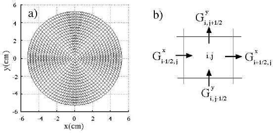
Figure 10: a) Initial position of the elements for the lagrangian simulation for the medium cap; b) Sketch of one cell and the corresponding horizontal and vertical fluxes for the Godunov scheme.

References

- [Anderson & Jackson 1992] Anderson, K. G. & Jackson, R. 1992 A comparison of the solutions of some proposed equations of motion of granular materials for fully developed flow down inclined planes. J. Fluid Mech. 241, 145–168.
- [Ancey et al 1996] Ancey, C., Coussot, P. & Evesque, P. 1996 Examination of the possibility of a fluid-mechanics treatment of dense granular flows. Mech. Cohesive-Frictional Mater. 1, 385–403.
- [Azanza et al 1999] Azanza, E., Chevoir, F. & Moucheront, P. 1999 Experimental study of collisional granular flows down an inclined plane. J. Fluid Mech. 400, 199–227.
- [Baumberger et al 1994] Baumberger, T., Heslot, F. & Perrin, B. 1994 Crossover from creep to inertial motion in friction dynamics. Nature 367, 544-546.
- [Bouchaud et al 1994] Bouchaud, J. P., Cates, M., Prakash, J. R. & Edwards, S. F. 1994 A model for the dynamics of sandpile surfaces. J. Phys. France I 4, 1383–1410.
- [Boutreux et al 1998] Boutreux, T., Raphael, E. & de Gennes, P. G. 1998 Surface flows of granular material: a modified picture for thick avalanches. Phys. Rev. E 58, 4692–4700.
- [Daerr & Douady 1999] Daerr, A. & Douady, S. 1999 Two types of avalanche behavior in granular media. Nature 399, 241–243.
- [Daerr 2001] Daerr, A. 2001 Dynamical equilibrium of avalanches on a rough plane. Phys. Fluids 13, 2115-2124.
- [Davis 1988] Davis, S.F. 1988 Simplified second order Godunov type methods. SIAM J. Sci. Stat. Comp. 9, 445–473.
- [Douady et al 1999] Douady, S., Andreotti, B. & Daerr, A. 1999 On granular surface flow equations. Eur. Phys. J. B 11, 131–142.
- [Ertas et al 2001] Ertas, D., Grest, G. S., Halsey, T. H., Levine, D. & Silbert, E. 2001 Gravity-driven dense granular flows. preprint cond-mat/0005051
- [Godunov 1959] Godunov, S. K. 1959 A finite difference method for the numerical computation of discontinuous solutions of the equations of fluid dynamics. Math. Sb. 47, 357–393.
- [Goldhirsch 1999] Goldhirsch, I. 1999 Scales and kinetics of granular flows. Chaos 9, 659–672.
- [Grandin 1986] Grandin, H. 1986 Fundamentals of the finite element method. New York Macmillan, London.
- [Gray et al 1999] Gray, J. M. N. T., Wieland, M. & Hutter, K. 1999 Gravity-driven free surface flow of granular avalanches over complex basal topography. Proc. R. Soc. Lond. A 455, 1841–1874.
- [Greve & Hutter 1993] Greve, R. & Hutter, K. 1993 Motion of a granular avalanche in a convex and concave curved chute: experiments and theoretical predictions. Phil. Trans. R. Soc. Lond. A 342, 573–600.
- [Greve et al 1994] Greve, R., Koch, T. & Hutter, K. 1994 Unconfined flow of granular avalanches along a partly curved surface: I. Theory . Proc. R. Soc. Lond. A 445, 399–413.
- [Haff 1983] Haff, P. K. 1983 Grain flow as a fluid-mechanical phenomenon. J. Fluid Mech. 134, 401–430.
- [Harten et al 1983] Harten A., Lax, P. D. & van Leer, B. 1983 On upstream differencing and Godunov type schemes for hyperbolic conservation laws. SIAM Review 25, 33–61.
- [Heinrich et al 2001] Heinrich, P., Boudon, G., Komorowski, J. C., Sparks, S. & Herd, H. 2001 Numerical simulation of the December 1997 debris avalanche in Montserrat, Lesser Antilles preprint.
- [Heslot et al 1994] Heslot, F., Baumberger, T., Perrin, B., Caroli, B. & Caroli, C. 1994 Creep, stick-slip, and dry-friction dynamics: experiments and a heuristic model. Phys. Rev. E 49, 4973-4987.
- [Hungr & Morgenstern 1984] Hungr, O. & Morgenstern, N. R. 1984 Experiments on the flow behavior of granular materials at high velocity in an open channel. Géotechnique 34, 405–413.
- [Ishida & Shirai 1979] Ishida, M. & Hirai, T. 1979 Velocity distributions in the flow of solid particles in an inclined open channel. J. Chem. Eng. Japan 12, 46–50.
- [Johnson et al 1990] Johnson, P. C., Nott, P. & Jackson, R. 1990 Frictional-collisional equations of motion for particulate flows and their application to chutes. J. Fluid Mech. 210, 501–535.
- [Koch et al 1994] Koch, T., Greve, R. & Hutter, K. 1994 Unconfined flow of granular avalanches along a partly curved surface: II. Experiments and numerical simulations. Proc. R. Soc. Lond. A 445, 415–435.
- [Lun et al 1984] Lun, C. K. K., Savage, S. B., Jeffrey, D. J. & Chepurniy, N. 1984 Kinetic theories for granular flow: inelastic particles in Couette flow and slightly inelastic particles in a general flowfield. J. Fluid Mech. 140, 223–256.
- [Mills et al 1999] Mills, P., Loggia, D. & Tixier, M. 1999 Model for a stationary dense granular flow along an inclined wall. Europhys. Lett. 45, 733–738.
- [Mills et al 2000] Mills, P.,Tixier, M. & Loggia, D. 2000 Influence of roughness and dilatancy for dense granular flow along an inclined wall. Eur. Phys. J. E 1, 5–8.
- [Naaim et al 1997] Naaim, M., Vial, S. & Couture, R. 1997 Saint Venant approach for rock avalanches modeling. In Multiple scale analyses and coupled physical systems: Saint Venant Symposium (Presse de l’ cole Nationale des Ponts et chaussees, Paris, 1997).
- [Nasuno et al 1997] Nasuno, S., Kudrolli, A. & Gollub, J.P. 1997 Friction in granular layers: hysteresis and precursors. Phys. Rev. Lett. 79, 949–953.
- [Nott & Jackson 1992] Nott, P. & Jackson, R. 1992 Frictional-collisional equations of motion for granular materials and their application to flow in aerated chutes. J. Fluid Mech. 241, 125–144.
- [Pouliquen & Renaut 1996] Pouliquen, O. & Renaut, N. 1996 Onset of granular flows on an inclined rough surface: dilatancy effects. J. Phys. II France 6, 923–935.
- [Pouliquen 1999a] Pouliquen, O. 1999 Scaling laws in granular flows down rough inclined planes. Phys. Fluids 11, 542–548.
- [Pouliquen 1999b] Pouliquen, O. 1999 On the shape of granular fronts down rough inclined planes. Phys. Fluids 11, 1956–1958.
- [Prochnow et al 2000] Prochnow, M., Chevoir, F. & Albertelli, M. 2000 Dense granular flows down a rough inclined plane. In Proceedings, XIIIth International Congress on Rheology, Cambridge, UK (2000)
- [Rajchenbach 2000] Rajchenbach, J. 2000 Granular flows. Advances in Physics 49, 229–256.
- [St Venant 1971] de Saint-Venant, A. J. C. 1871 Th orie du mouvement non-permanent des eaux, avec application aux crues des rivi res et a l’introduction des mar es dans leur lit. C. R. Acad. Sc. Paris 73, 147–154.
- [Sansoni et al 1999] Sansoni, G., Carocci, M & Rodella, R. 1999 3D vision based on the combination of gray code and phase shift light projection: analysis and compensation of the systematic errors. Appl. Opt. 31, 6565–6573.
- [Savage 1983] Savage, S. B. 1983 Granular flows down rough inclines-review and extension. In Advances in Micromechanics of granular materials, edited by J. T. Jenkins and M. Satake et al (Elsevier, Amsterdam, 1983)
- [Savage & Hutter 1989] Savage, S. B. & Hutter, K. 1989 The motion of a finite mass of granular material down a rough incline. J. Fluid Mech. 199, 177–215.
- [Savage 1998] Savage, S. B. 1998 Analyses of slow high-concentration flows of granular materials. J. Fluid Mech. 377, 1–26.
- [Suzuki & Tanaka 1971] Suzuki, A. & Tanaka, T. 1971 Measurement of flow properties of powders along an inclined plane. Ind. End. Chem. Fundam. 10, 84–91.
- [Vallance 1994] Vallance, J. W. 1994 Experimental and field studies related to the behavior of granular mass flows and the characteristics of their deposits, Ph.D Thesis (Michigan Technological University.
- [Wielandet al 1999] Wieland, J. M., Gray, J. M. N. T. & Hutter, K. 1999 Channelized free-surface flow of cohesionless granular avalanches in a chute with shallow lateral curvature. J. Fluid Mech. 392, 73–100.