Influence of disorder on the ferromagnetism in diluted magnetic semiconductors.

Abstract

Influence of disorder in the concentration of magnetic Mn²⁺ ions on the ferromagnetic phase transition in diluted (III,Mn)V semiconductors is investigated analytically. The regime of small disorder is addressed, and the enhancement of the critical temperature by disorder is found both in the mean field approximation and from the analysis of the zero temperature spin stiffness. Due to disorder, the spin wave fluctuations around the ferromagnetically ordered state acquire a finite mass. At large charge carrier band width, the spin wave mass squared becomes negative, signaling the breakdown of the ferromagnetic ground state.

I Introduction

The prospects of application in spin electronic devices inspired much experimental [1] and theoretical [2, 3, 4, 5, 6] activity in studying the itinerant ferromagnetism in (III,Mn)V diluted magnetic semiconductors. The theoretical efforts led to much understanding of the basic features of that material system, providing a mean-field description and reasonable estimates of the ferromagnetic phase transition temperature from the spin-wave stiffness [2, 4] .

There are two important issues, however, that have not been completely understood so far, namely, the role of disorder and interactions between the mobile charge carriers (holes) in the ferromagnetic phase transition. In this paper, we address the issue of disorder in the concentration of magnetic Mn-dopants. The role of disorder is two-fold. On one hand, the variation in the Mn-concentration creates regions with local concentration of Mn-spins higher than the average. These regions tend to be magnetically polarized by itinerant carriers at higher temperatures than the phase transition temperature for the homogeneous system. The latter should lead to higher transition temperatures in the disordered system. On the other hand, the disorder leads to localization of the mobile charge carriers, thus hampering the onset of long range magnetic correlations, which would lower the transition temperature in the disordered system. Presumably, the first effect prevails, if the localization of holes is weak, whereas in the case of strongly localized carriers (strong disorder) the second effect takes over. The enhancement of the transition temperature in disordered systems has been reported in recent theoretical investigations by R. N. Bhatt and M. Berciu [3], and J. Schliemann et al [4]. The results of this paper qualitatively agree with [3, 4]. However, the region of strong localization of the charge carries, where the suppression of the critical temperature presumably takes place is not addressed here.

II Theoretical model and approximations

The microscopic description of the itinerant ferromagnetism in (III,Mn)V semiconductors is given by the Kondo lattice Hamiltonian. In contrast to the Kondo system, in the system under consideration the concentration of the charge carriers (mobile holes in the valence band) $p$ is much lower than the concentration of the Mn-spins $N_{Mn}$. The latter rules out the Kondo effect. Moreover, the $pd$ exchange coupling $J$ is larger than the Fermi energy [1, 2]. As a result, in the ferromagnetic state, the charge carriers (holes) are completely spin polarized.

A hole magnetically polarizes the Mn spins in its vicinity, thus forming a magnetic polaron. Close to the ferromagnetic phase transition there is a large correlation length in the Mn spin system, and the dynamics of mobile holes is much faster than the dynamics of Mn spins. In this case, the magnetic polarization cloud created by a hole stays for some relaxation time $\tau_{Mn}$ after the hole has left the region. The linear size of the polaron cloud can be estimated as $R\sim v\tau_{Mn}$, where $v$ is the velocity of the hole (the motion of the hole inside the polarized region is assumed to be ballistic). The condition of low hole concentration, $p\ll N_{Mn}$, [1, 2] implies that there is no more than one mobile hole polarizing the cloud at a given moment of time.

Therefore, the physical picture close to the phase transition point is that of slowly relaxing Mn-clusters (or polaronic clouds) polarized by the spins of mobile holes. The hopping of holes establishes long range correlations between the clusters. Due to the randomness in the Mn concentration, the number of Mn-spins in each cluster is randomly distributed around some average value. This picture is conveyed in the mathematical model below.

The model consists of mobile holes moving on a lattice with sites $i$. The holes are represented by the fermionic operators $\hat{a}^{+}_{i\sigma},\hat{a}_{i\sigma}$. The other ingredient is a system of Mn-spins $5/2$ distributed randomly over a lattice with sites $j$. Since the concentration of Mn spins is larger then the concentration of holes [1, 2], there are many Mn-sites within a unit cell of the hole lattice. A hole polarizes Mn-spins in its vicinity. Because of the randomness in the Mn distribution, the number of polarized spins around the site $i$ is random.

The Hamiltonian of the model writes

$$\hat{H}=-t\sum_{<i,i^{\prime}>}(\hat{a}^{+}_{i\sigma}\hat{a}_{i^{\prime}\sigma}+h.c.)+J\sum_{i}\sum_{j=1}^{N_{i}}{\bf\hat{s}}_{i}{\bf\hat{S}}_{ji}.$$ (1)

The first term describes the nearest neighbor hopping of holes. In this paper, a simplified one-band hole dispersion is used instead of the six-band model relevant for (Ga,Mn)As. [2] Whereas the one-band model is insufficient to give a quantitative prediction for the critical temperature, it reproduces the basic qualitative features of the hole system, including the effects of disorder [3, 6]. In the interaction term, ${\bf\hat{s}}_{i}=\hat{a}^{+}_{i\alpha}{\bf\sigma}_{\alpha\beta}\hat{a}_{i\beta}$ describes the spin of a hole on site $i$, and the operators ${\bf\hat{S}}_{ji}$ describe the Mn-spins in the vicinity of site $i$. The interaction term is written under the assumption of a rectangular hole wave function, so that the constant $J$ does not depend on the distance between the hole and the Mn-spin within the interaction range.

There is a total of $N_{i}$ Mn-spins polarized by the hole at site $i$. The number $N_{i}$ is taken to be random gaussian distributed with mean $N_{p}$ and variation $\Delta/\sqrt{N_{p}}$

$$P(N_{i})\propto\exp\left[-\frac{N_{p}(N_{i}-N_{p})^{2}}{2\Delta^{2}}\right].$$ (2)

In the experimental system the average $N_{p}$ is usually small [1], $N_{p}\sim 3$. Therefore, the Poissonian distribution is actually more appropriate to describe the disorder in $N_{i}$. We take the Gaussian distribution for the sake of technical convenience. The case of the Poissonian distribution of $N_{i}$ is left for future investigations. To restrict the influence of the unphysical region of negative $N_{i}$, the condition $\Delta\ll N_{p}$ is adopted in numerical evaluations below (see Section III).

To deal with disorder, we employ the replica-trick. In the replicated partition function for the Hamiltonian (1), the interaction term is represented by $\exp[-J\sum_{i}\sum_{j=1}^{N_{i}}\sum_{a=1}^{n}\int_{0}^{\beta}d\tau{\bf s}^{a\tau}_{i}{\bf S}^{a\tau}_{ji}]$, where $a$ denotes the replica-index, and $\tau$ denotes the imaginary time. We decouple the interaction term by the Hubbard–Stratonovich transformation, introducing decoupling fields for the magnetization of Mn-spins and hole-spins. After the decoupling, the interaction part of the partition function assumes the form

$$\exp[-J\sum_{i}\sum_{j=1}^{N_{i}}\sum_{a=1}^{n}\int_{0}^{\beta}d\tau{\bf s}^{a\tau}_{i}{\bf S}^{a\tau}_{ji}]\propto\int\prod_{<i,j>}D[{\bf X}_{ij}^{a\tau}]D[{\bf Y}_{ij}^{a\tau}]$$ (3)

$$\exp\left[-\sum_{a}\int_{0}^{\beta}d\tau\sum_{<i,j>}\frac{{\bf X}_{ij}^{a\tau}{\bf Y}_{ij}^{a\tau}}{J}+\sum_{a}\int_{0}^{\beta}d\tau\sum_{<i,j>}\left\{{\bf X}_{ij}^{a\tau}{\bf S}_{ij}^{a\tau}-{\bf Y}_{ij}^{a\tau}{\bf s}_{i}^{a\tau}\right\}\right].$$ (4)

The term $\sum_{<i,j>}{\bf{X}}_{ij}^{a\tau}{\bf{S}}_{ij}^{a\tau}$ describes the Mn-spins in the cluster around site $i$ under the influence of the effective field created by mobile holes. ${\bf{X}}_{ij}^{a\tau}$ is the effective field created by a hole at site $i$ and acting on the Mn-spin on site $j$. For a rectangular form of the hole wave function, we replace ${\bf X}_{ij}^{a\tau}={\bf X}_{i}^{a\tau}\ \forall j=\overline{1,N_{i}}$. In what follows we use the Holstein–Primakoff representation for the total spin of the cluster [7], ${\bf\Xi}_{i}\equiv\sum_{j=1}^{N_{i}}{\bf S}_{ij}$,

$$\Xi_{i}^{z} = N_{i}S-\hat{b}^{+}_{i}\hat{b}_{i},$$ (5)

$$\Xi_{i}^{+} = (\sqrt{2N_{i}S-\hat{b}^{+}_{i}\hat{b}_{i}})\hat{b}_{i},$$ (6)

$$\Xi_{i}^{-} = \hat{b}_{i}^{+}(\sqrt{2N_{i}S-\hat{b}^{+}_{i}\hat{b}_{i}}),$$ (7)

where $\hat{b}_{i}^{+},\hat{b}_{i}$ are bosonic creation and annihilation operators, describing the excitations around the ordered state of the cluster. There is a constraint on the number of bosons in each cluster $\langle\hat{b}_{i}^{+}\hat{b}_{i}\rangle\leq 2N_{i}S$, $S=5/2$. The further calculations are carried out in the quadratic approximation in the bosonic fields $\hat{b}_{i}^{+},\hat{b}_{i}$ , so we replace in the square root $\sqrt{2N_{i}S-\hat{b}^{+}_{i}\hat{b}_{i}}\approx\sqrt{2N_{i}S}$.

Finally, under the assumption of the rectangular form of the hole’s wave function, we approximate the effective field exerted by the Mn-cluster on the hole at the site $i$, $\sum_{j=1}^{N_{i}}{\bf Y}_{ij}^{a\tau}{\bf s}_{i}^{a\tau}\approx N_{i}{\bf Y}_{i}^{a\tau}{\bf s}_{i}^{a\tau}$. Under the approximations above, the replicated partition function of the model (1) can be written as

$$Z^{n}\approx\int D[\bar{a}_{i\sigma}^{a\tau}]D[a_{i\sigma}^{a\tau}]D[\bar{b}_{i\sigma}^{a\tau}]D[b_{i\sigma}^{a\tau}]D[{\bf X}_{i}^{a\tau}]D[{\bf Y}_{i}^{a\tau}]\exp\left[\sum_{a=1}^{n}\sum_{i}\int_{0}^{\beta}d\tau\left\{\sum_{\sigma=\uparrow,\downarrow}\bar{a}_{i\sigma}^{a\tau}(-\partial_{\tau}+\mu)a_{i\sigma}^{a\tau}\right.\right.$$ (9)

$$\left.+\bar{b}_{i}^{a\tau}(-\partial_{\tau}-X_{zi}^{a\tau})b_{i}^{a\tau}\right\}+t\sum_{<i,i^{\prime}>}\sum_{a=1}^{n}\sum_{\sigma}(\bar{a}^{a\tau}_{i\sigma}a^{a\tau}_{i^{\prime}\sigma}+\bar{a}^{a\tau}_{i^{\prime}\sigma}a^{a\tau}_{i\sigma})$$ (10)

$$-\sum_{i}N_{i}\sum_{a}\int_{0}^{\beta}d\tau\left\{Y_{zi}^{a\tau}({\bf\bar{a}}_{i}^{a\tau}{\bf\sigma}^{z}{\bf a}_{i}^{a\tau})+SX_{zi}^{a\tau}-(X_{zi}^{a\tau}Y_{zi}^{a\tau})/J\right\}$$ (11)

$$+\sum_{i}\sum_{a=1}^{n}\int_{0}^{\beta}d\tau\left\{\sqrt{2SN_{i}}(X_{i+}^{a\tau}\bar{b}_{i}^{a\tau}+X_{i-}^{a\tau}b_{i}^{a\tau})-N_{i}\left(Y_{i+}^{a\tau}({\bf\bar{a}}_{i}^{a\tau}{\bf\sigma}^{-}{\bf a}_{i}^{a\tau})+Y_{i-}^{a\tau}({\bf\bar{a}}_{i}^{a\tau}{\bf\sigma}^{+}{\bf a}_{i}^{a\tau})\right)\right.$$ (12)

$$\left.\left.-N_{i}(X_{i+}^{a\tau}Y_{i-}^{a\tau}+X_{i-}^{a\tau}Y_{i+}^{a\tau})/J\right\}\right].$$ (13)

Here $\bar{a}_{i\sigma}^{a\tau},a_{i\sigma}^{a\tau}$ denote the Grassman fields associated with the mobile holes, and $\bar{b}_{i}^{a\tau},b_{i}^{a\tau}$ denote the complex variables associated with the bosonic operators $\hat{b}_{i}^{+},\hat{b}_{i}$. We introduced the spinors ${\bf a}_{i}^{a\tau},{\bf\bar{a}}_{i}^{a\tau}$, which are formed as follows, ${\bf a}_{i}^{a\tau}\equiv(a_{i\uparrow}^{a\tau},a_{i\downarrow}^{a\tau})^{T}$, ${\bf\bar{a}}_{i}^{a\tau}=({\bf a}_{i}^{a\tau})^{+}$.

The partition function (13) is analyzed on the mean field level. The mean field approximations include neglecting the transverse fluctuations of spins (only $z$-components of fields are considered), and a static and spatially homogeneous ansatz for the fields $X_{iz}^{a\tau}\approx X^{a}$, $Y_{iz}^{a\tau}\approx Y^{a}$. The averaging over the disorder with the distribution (2) results in a term in the effective free energy that mixes different replicas and looks as

$$-\frac{\Delta^{2}}{2N_{p}}\sum_{i}\sum_{a,b=1}^{n}Y^{a}Y^{b}\int_{0}^{\beta}d\tau d\tau^{\prime}({\bf\bar{a}}_{i}^{a\tau}{\bf\sigma}^{z}{\bf a}_{i}^{a\tau})({\bf\bar{a}}_{i}^{b\tau^{\prime}}{\bf\sigma}^{z}{\bf a}_{i}^{b\tau^{\prime}}).$$ (14)

The structure of term (14) is typical for the replica treatment of the Anderson localization problem [8]. Under the mean field approximations made above, the strength of the disorder in the effective localization problem is proportional to the mean field value of the squared magnetization in the Mn-clusters $Y^{a}Y^{b}$. Therefore, expression (14) accounts for the localization of holes by the random potential from the frozen Mn-clusters. The treatment of (14) repeats the nonlinear sigma-model approach for the Anderson localization [8]. The term is decoupled in the following fashion

$$\exp\left[-\frac{\Delta^{2}}{2N_{p}}\sum_{i}\sum_{a,b=1}^{n}Y^{a}Y^{b}\int_{0}^{\beta}d\tau d\tau^{\prime}({\bf\bar{a}}_{i}^{a\tau}{\bf\sigma}^{z}{\bf a}_{i}^{a\tau})({\bf\bar{a}}_{i}^{b\tau^{\prime}}{\bf\sigma}^{z}{\bf a}_{i}^{b\tau^{\prime}})\right]\propto$$ (15)

$$\int d{\bf Q}_{i}^{a\tau,b\tau^{\prime}}d{\bf Q}_{i}^{b\tau^{\prime},a\tau}\exp\left[-\frac{N_{p}}{2\Delta^{2}}\sum_{i}\sum_{a,b=1}^{n}\left\{Y^{a}Y^{b}\int_{0}^{\beta}d\tau d\tau^{\prime}[{\bf Q}_{i}^{a\tau,b\tau^{\prime}}(\sigma^{z}\otimes\sigma^{z}){\bf Q}_{i}^{b\tau^{\prime},a\tau}\right.\right.$$ (16)

$$\left.\left.+i\frac{Y^{a}Y^{b}}{2}\left\{{\bf Q}_{i}^{a\tau,b\tau^{\prime}}(\sigma^{z}\otimes\sigma^{z}){\bf\bar{a}}_{i}^{b\tau^{\prime}}{\bf a}_{i}^{a\tau}+{\bf\bar{a}}_{i}^{a\tau}{\bf a}_{i}^{b\tau^{\prime}}(\sigma^{z}\otimes\sigma^{z}){\bf Q}_{i}^{b\tau^{\prime},a\tau}\right\}]-\frac{\beta^{2}}{2}\log(Y^{a}Y^{b})\right\}\right],$$ (17)

where ${\bf Q}_{i}^{a\tau,b\tau^{\prime}}$ is a matrix in the spin space with elements $(Q_{i}^{a\tau,b\tau^{\prime}})_{\sigma\sigma^{\prime}}$. Here we concentrate only on the mean field solution for the matrix ${\bf Q}$. After Fourier transformation with respect to imaginary times $\tau,\tau^{\prime}$, the mean field ansatz reads

$${\bf Q}_{i}^{a\omega,b\omega^{\prime}}={\bf\Lambda}^{a}_{\omega}sign(\omega)\delta_{\omega\omega^{\prime}}\delta_{ab}.$$ (18)

Neglecting the transverse spin fluctuations, we assume a diagonal structure of the matrix ${\bf\Lambda}_{\omega}$ in the spin sector

$${\bf\Lambda}^{a}_{\omega}=\left(\begin{array}[]{cc}\Lambda_{\uparrow\uparrow}^{a,\omega}&0\\ 0&\Lambda_{\downarrow\downarrow}^{a,\omega}\end{array}\right).$$ (19)

Finally, the mean field partition function acquires the form

$$\langle Z^{n}\rangle_{MF}=\int D[\bar{a}_{i\sigma}^{a\tau}]D[a_{i\sigma}^{a\tau}]D[\bar{b}_{i\sigma}^{a\tau}]D[b_{i\sigma}^{a\tau}]\exp\left[N\sum_{a=1}^{n}\sum_{\omega_{n}}\int d^{d}k\left\{\bar{a}_{k\uparrow}^{a\omega}[i\omega_{n}+\mu-\epsilon_{k}-N_{p}Y^{a}\right.\right.$$ (20)

$$+iY^{a}\Lambda_{\uparrow\uparrow}^{a\omega}sign(\omega_{n})+\beta\frac{\Delta^{2}}{N_{p}}Y^{a}\sum_{b=1}^{n}(Y^{b}X^{b}/J-SX^{b})]a_{k\uparrow}^{a\omega}$$ (21)

$$\left.+\bar{a}_{k\downarrow}^{a\omega}[i\omega_{n}+\mu-\epsilon_{k}+N_{p}Y^{a}+iY^{a}\Lambda_{\downarrow\downarrow}^{a\omega}sign(\omega_{n})-\beta\frac{\Delta^{2}}{N_{p}}Y^{a}\sum_{b=1}^{n}(Y^{b}X^{b}/J-SX^{b})]a_{k\downarrow}^{a\omega}\right\}$$ (22)

$$+\sum_{a=1}^{n}\sum_{\omega_{n}}\sum_{i=1}^{N}\left\{\bar{b}_{i}^{a\omega}(-i\omega_{n}-X^{a})b_{i}^{a\omega}\right\}-\frac{NN_{p}}{2\Delta^{2}}\sum_{a=1}^{n}(Y^{a})^{2}\sum^{F}_{\omega}\left\{(\Lambda_{\uparrow\uparrow}^{\omega})^{2}+(\Lambda_{\downarrow\downarrow}^{\omega})^{2}\right\}$$ (23)

$$+\beta NN_{p}\sum_{a=1}^{n}\left\{SX^{a}-X^{a}Y^{a}/J\right\}+\frac{N\beta^{2}\Delta^{2}}{2N_{p}}\sum_{a,b=1}^{n}\left\{S^{2}X^{a}X^{b}+X^{a}X^{b}Y^{a}Y^{b}/J^{2}\right.$$ (24)

$$\left.\left.-2SX^{a}X^{b}Y^{b}/J\right\}\right].$$ (25)

Here the sum over the frequencies $\omega_{n}$ denote the sum over the fermionic Matsubara frequencies for the fields $\bar{a},a$, and the sum over the bosonic Matsubara frequencies for the fields $\bar{b},b$. $N$ denotes the total number of sites $i$ in the lattice. The exponent in (25) is quadratic in the bosonic ($\bar{b},b$) and the fermionic ($\bar{a},a$) variables, hence the bosons and fermions can be intergrated out. When integrating out the bosons, the restriction on the bosonic occupation number $n_{b}\leq 2N_{p}S$ is explicitely taken into account.

III Mean field equations and their solutions

We adopt the replica symmetric mean field ansatz for the fields $Y^{a}=Y$, $X^{a}=X$, $\Lambda^{a\omega}_{\sigma\sigma}=\Lambda^{\omega}_{\sigma\sigma}\ \forall a=\overline{1,n}$. In the replica symmetic approximation, the terms in (25) involving the sum over different replicas give no contribution to the mean field equations in the replica limit $n\rightarrow 0$.

Further, we change from the integral over wave vectors to an integral over the energies $\int d^{d}k...=\int\rho_{d}(\epsilon)d\epsilon$, where $\rho_{d}(\epsilon)$ denotes the d-dimensional density of states (DoS). Under the above approximations, the following mean field equations have been obtained

$$Y=\frac{J}{N_{p}}\frac{\sum_{l=0}^{(5N_{p}-1)/2}\left(\frac{5}{2}N_{p}-l\right)\sinh\left[\beta\left(\frac{5}{2}N_{p}-l\right)X\right]}{\sum_{l=0}^{(5N_{p}-1)/2}\cosh\left[\beta\left(\frac{5}{2}N_{p}-l\right)X\right]}.$$ (26)

Here $Y$ is the average magnetization of a single Mn-spin in units of $J$. Mn-spins are magnetically polarized by the effective field of the holes $X$, which is reflected by the RHS of Eq. (26). The average magnetization of a hole $X$ (in units of $J$) is given by the equation

$$X=\frac{J}{\Delta^{2}}YT\sum^{F}_{\omega_{n}}\left\{(\Lambda_{\uparrow\uparrow}^{\omega})^{2}+(\Lambda_{\downarrow\downarrow}^{\omega})^{2}\right\}$$ (27)

$$+JT\sum_{\omega_{n}}^{F}\int_{-W}^{W}\rho(\epsilon)d\epsilon\left\{\frac{1}{i\omega_{n}+\mu-\epsilon+N_{p}Y+iY^{2}\Lambda_{\downarrow\downarrow}^{\omega}sign(\omega_{n})}\right.$$ (28)

$$\left.-\frac{1}{i\omega_{n}+\mu-\epsilon-N_{p}Y+iY^{2}\Lambda_{\uparrow\uparrow}^{\omega}sign(\omega_{n})}\right\}.$$ (29)

Eq. (29) describes the magnetic polarization of itinerant carriers (holes) in the effective field $N_{p}Y$ created by Mn-spins. Disorder enters Eq. (29) through the disorder strength $\Delta$ and the fields $\Lambda_{\sigma\sigma}^{\omega}$ which, on the mean field level, are proportional to the inverse mean free time for holes. At zero temperature, the inverse mean free time for holes with a spin projection $\sigma$ is given by $1/\tau_{\sigma}=2Y^{2}\Lambda_{\sigma\sigma}^{0}$. Since only the scattering by frozen magnetic moments is taken into account on the mean field level, the influence of disorder disappears completely in the paramagnetic phase. In the paramagnetic phase, the scattering by dynamical magnetic fluctuations in Mn spin clusters affects the hole motion. The account for that effect is beyond the static mean field approximation adopted here. The analysis of that and other fluctuation effects beyond the mean field approximation is left for future investigations.

Equations for the mean field values of $\Lambda_{\sigma\sigma}^{\omega}$ can be written as

$$\Lambda_{\sigma\sigma}^{\omega}=\frac{\Delta^{2}}{N_{p}}\int_{-W}^{W}\rho(\epsilon)d\epsilon\frac{i\ sign(\omega_{n})}{i\omega_{n}+\mu-\epsilon\mp N_{p}Y+iY^{2}\Lambda_{\sigma\sigma}^{\omega}\ sign(\omega_{n})}.$$ (30)

The upper sign in the denominator corresponds to $\sigma=\uparrow$ and the lower sign corresponds to $\sigma=\downarrow$. For $d=2,3$, I replace the density of states $\rho_{d}(\epsilon)$ in (29), (30) by a constant average density of states $\rho_{d}(\epsilon)=\rho$. The example of a spherically symmetric band $\epsilon({\bf k})=-W\cos(|{\bf k}|)$ shows that for large $W$, the contribution of the singularity of the DoS near the band edge $\epsilon=W$ is small in both two and three dimensions, hence the above replacement is justified. Upon that replacement, the integrals over the energy $\epsilon$ in Eqs. (29), (30) can be performed explicitely, and the equations for $X$ and $\Lambda_{\sigma\sigma}$ assume the form

$$X=J\rho T\sum^{F}_{\omega_{n}>0}\log\left|\frac{[(W-\mu+N_{p}Y)^{2}+(\omega_{n}+Y^{2}\Lambda_{\uparrow\uparrow}^{\omega})^{2}][(W+\mu+N_{p}Y)^{2}+(\omega_{n}+Y^{2}\Lambda_{\downarrow\downarrow}^{\omega})^{2}]}{[(W+\mu-N_{p}Y)^{2}+(\omega_{n}+Y^{2}\Lambda_{\uparrow\uparrow}^{\omega})^{2}][(W-\mu-N_{p}Y)^{2}+(\omega_{n}+Y^{2}\Lambda_{\downarrow\downarrow}^{\omega})^{2}]}\right|$$ (31)

$$+\frac{J}{\Delta^{2}}YT\sum^{F}_{\omega_{n}}\left\{(\Lambda_{\uparrow\uparrow}^{\omega})^{2}+(\Lambda_{\downarrow\downarrow}^{\omega})^{2}\right\}.$$ (32)

$$\Lambda_{\uparrow\uparrow}^{\omega}=\rho\frac{\Delta^{2}}{N_{p}}\left[\arccos\left(\frac{N_{p}Y-W-\mu}{|N_{p}Y-W-\mu+i(\omega_{n}+Y^{2}\Lambda_{\uparrow\uparrow}^{\omega})|}\right)\right.$$ (33)

$$\left.-\arccos\left(\frac{N_{p}Y+W-\mu}{|N_{p}Y+W-\mu+i(\omega_{n}+Y^{2}\Lambda_{\uparrow\uparrow}^{\omega})|}\right)\right],\ \omega_{n}>0,$$ (34)

$$\Lambda_{\downarrow\downarrow}^{\omega}=\rho\frac{\Delta^{2}}{N_{p}}\left[\arccos\left(\frac{N_{p}Y-W+\mu}{|N_{p}Y-W+\mu+i(\omega_{n}+Y^{2}\Lambda_{\downarrow\downarrow}^{\omega})|}\right)\right.$$ (35)

$$\left.-\arccos\left(\frac{N_{p}Y+W+\mu}{|N_{p}Y+W+\mu+i(\omega_{n}+Y^{2}\Lambda_{\downarrow\downarrow}^{\omega})|}\right)\right],\ \omega_{n}>0.$$ (36)

We analyze the mean field phase diagram by solving numerically mean field equations (26), (32)–(36), taking the parameters close to those of (Ga,Mn)As. The exchange constant for (Ga,Mn)As equals $J_{0}\approx 55$ meV nm³. The constant $J_{0}$ is adopted in the model with a $\delta$-like interaction between a hole and Mn-spins of the form [2]

$$H_{int}=-J_{0}\sum_{i,I}{\bf S}_{I}{\bf s}_{i}\delta({\bf r}_{i}-{\bf R}_{I}).$$ (37)

Comparison of (37) with the interaction term in (1) for the homogeneous case $N_{i}=N_{p}$ gives the relation $J=J_{0}/N_{p}$. The number $N_{p}$ can be evaluated as $N_{p}\sim N_{Mn}/p$. For $N_{Mn}=1.0$ nm^-3, $p=0.35$ nm^-3 we infer $N_{p}\sim(N_{Mn}/p)\approx 3$. For the simplified band structure adopted here, the average density of states $\rho$ and the width of the band $W$ cannot be directly obtained from experimental data. The chemical potential is fixed by the condition of constant concentration of holes $p$, or constant filling factor $\nu$ of the charge carrier lattice $i$ of the model (1).

The mean field equations (26), (32) – (36) were solved numerically for $J=10$ meV, and different values of $N_{p}$, $\rho$, $W$, $\nu$, and $\Delta$. In all cases we found that the critical temperature increases with disorder strength $\Delta$. The temperature dependence of the magnetizations of holes $X$ and Mn-spins $Y$ for the set of parameters $J=10$ meV nm³, $N_{p}=5$, $W=100$ meV, $\rho=0.01$ meV^-1 nm^-3, $\nu=0.25$ and different values of disorder strength $\Delta$ is shown in Fig. 1.

IV Spin waves in a disordered ferromagnet

There are massless Goldstone modes in the ordered phase of a clean system – the spin waves. The zero temperature spin stiffness has been used in Ref. [4] to give an estimate for the critical temperature, which is much closer to experimental data than the mean field result in the regime of small concentration of charge carriers and large exchange coupling $J$ (as compared to the Fermi energy).

The spin wave excitations are described by bosonic fields $\bar{b},b$. In this section, we calculate the zero temperature dispersion of the spin-wave excitations around the saddle point (26) – (36) described above, and use the result to analyze qualitatively the influence of disorder on the critical temperature calculated from the spin wave stiffness. Since the role of disorder increases at low temperatures, the calculation of the zero temperature spin stiffness using the mean field description of the disorder effects (the fluctuations of the field $\bf Q$ are not taken into account) is perturbative in the disorder strength $\Delta$. It can be used only to describe the qualitative behavior of $T_{c}$. The zero temperature spin wave dispersion is given by

$$\Omega=Dq^{2}+m_{SW}^{2}.$$ (38)

The spin waves acquire a mass $m_{SW}$. Both $D$ and $\lambda$ also have imaginary parts that describe the attenuation of spin waves in a disordered system. At zero temperature, the approximate expression for the spin stiffness reads

$$D\approx\frac{2\pi\rho v_{F}^{2}}{3N_{p}S}\left(1+4\frac{\Delta^{2}}{N_{p}^{5}}\right),$$ (39)

where we neglected the imaginary part and assumed $\pi\rho\ll N_{p}J$, which is consistent with the regime of low concentration of holes. $v_{F}$ denotes the Fermi velocity. One can see from expression (39) that the spin stiffness grows with disorder strength $\Delta$ at small disorder. This in turn results in an increase of the critical temperature. The critical temperature can be estimated according to formula [4]

$$T_{c}\approx Dk^{2}_{D}$$ (40)

with the Debye wave vector $k_{D}=(6\pi^{2}N_{p})^{1/3}$.

The critical temperature versus the disorder strength $\Delta$ calculated in the mean field approximation is shown in Fig. 2. The critical temperature grows strongly with disorder. In contrast, the evaluation of the critical temperature from the spin wave stiffness (40) gives a much weaker dependence on the disorder.

The zero temperature mass of the spin wave excitations $m_{SW}$ is given by

$$m^{2}_{SW}\approx\frac{64\Delta^{2}J^{2}S}{N_{p}^{2}}\pi\rho(\Lambda^{0}_{\uparrow\uparrow}-\Lambda^{0}_{\downarrow\downarrow})-\frac{JS}{2\pi\Delta^{2}}\int d\omega\left\{(\Lambda^{\omega}_{\uparrow\uparrow})^{2}+(\Lambda^{\omega}_{\downarrow\downarrow})^{2}\right\},$$ (41)

where we neglected a small imaginary part. The dependence of the spin wave mass $m_{SW}^{2}$ on the hole bandwidth $W$ at two different sets of other parameters is shown in Fig. 3. At large bandwidth $W$, $m_{SW}^{2}$ becomes negative (see Fig. 3), which signals the breakdown of the collinear ferromagnetic order. The transition to negative $m_{SW}^{2}$ occurs at lower values of $W$ for a smaller average number of spins $N_{p}$ in a magnetic cluster.

Presumably, in the regime $m_{SW}^{2}<0$ the ground state is noncollinear. The existence of a noncollinear ground state in disordered (III,Mn)V semiconductors has been suggested recently [6].

V Summary and discussion

In this paper we investigated the influence of disorder on the critical temperature of an itinerant ferromagnet. The theoretical modeling in the regime close to the phase transition was based on the picture of magnetic polaronic clouds (magnetic clusters) with large relaxation time. The clusters are polarized by mobile holes hopping between them. The regime of small concentration of mobile holes considered here is relevant for the ferromagnetism in (III,Mn)V compounds. The disorder in the Mn concentration is naturally included as a random number of spins in each magnetic cluster. At the critical point, the clusters begin to percolate, developing infinite range magnetic correlations.

We found that the critical temperature grows with disorder, both in the mean field approximation and if calculated from the zero temperature spin stiffness. However, the influence of disorder turns out to be much stronger in the mean field evaluation of $T_{c}$ than by the estimation from the spin stiffness. In both approaches, disorder is taken into account perturbatively. In the mean field calculation, the perturbative treatment of disorder can be justified, if the critical temperature is high (which is the case in the experiment), and the localization is suppressed.

In contrast, the estimation of $T_{c}$ from the zero temperature spin stiffness is much less reliable. At zero temperature, the higher order localization corrections become important, and perturbative account for disorder may result in the underestimation of the disorder effect on the spin stiffness. The latter, in turn, leads to the underestimaiton of the influence of disorder on $T_{c}$. At the same time, the calculations of the spin stiffness correctly reflect the general tendency that the spin stiffness, and therefore the critical temperature, grows with disorder.

The physical reason for the increase of $T_{c}$ at weak disorder was proposed in Ref. [3]. In the disordered system, a mobile hole spends more time in the regions with higher Mn concentration, thus the effective magnetic coupling increases. However, at strong disorder, the critical temperature should eventually decrease because of localization of the charge carriers that mediate the magnetic correlations.

In this work we neglected the localization corrections that should make the motion of the holes diffusive. The work on this subject is in progress.

We thank A. H. MacDonald, J. Schliemann, J. König, and K. Scharnberg for useful discussions.

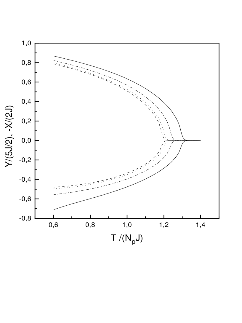
FIG. 1.: Relative magnetization of Mn-spins $Y/(JS)$ ($\geq 0$) and holes $-X/(2J)$ ($\leq 0$) versus temperature at different disorder strengths. The critical temperature increases with the disorder strength $\Delta$. In order of increasing $T_{c}$: $\Delta=0.1;1.0;2.0;3.0$. Other parameters: $J=10$ meV nm³, $N_{p}=5$, $W=100$ meV, $\rho=0.01$ meV^-1nm^-3, $\nu=0.25$.

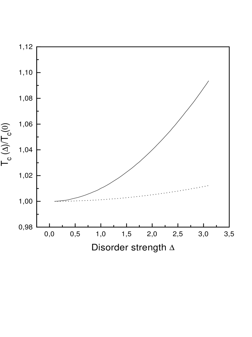
FIG. 2.: Relative change of the critical temperature with the strength of disorder $T_{c}(\Delta)/T_{c}(\Delta=0)$ as calculated from the mean field equations (solid line), and from the zero-T spin wave stiffness (dots). $J=10$ meV nm³, $N_{p}=5$, $W=100$ meV, $\rho=0.01$meV^-1nm^-3, $\nu=0.25$.

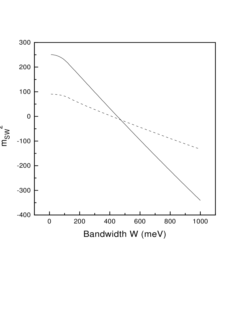
FIG. 3.: Zero temperature spin wave mass versus the bandwidth $W$. $J=10$ meV nm³, $N_{p}=5,\mu=0$, $\rho=1.0$ meV^-1 nm^-3. Solid line: $\Delta=0.5$. Dashed line: $\Delta=0.3$.

REFERENCES

- [1] H. Ohno, Science 281, 951 (1998); H. Ohno, J. of Magnetism and Magnetic Materials 200, 110 (1999); F. Matsukura, H. Ohno, A. Shen, and Y. Sugawara, Phys. Rev. B 57 R2037 (1998); H. Ohno, F. Matsukura, Sol. State Comm. 117, 179 (2001); T. Dietl, H. Ohno, Physica E 9, 185 (2001).
- [2] J. König, H.H. Lin, and A.H.MacDonald, Phys. Rev. Lett. 84, 5628 (2001), cond-mat/0010471; J. König, T. Jungwirth, A.H. MacDonald, cond-mat/0103116; M. Abolfath, T. Jungwirth, A.H. MacDonald, cond-mat/0103341.
- [3] X. Wan, R. N. Bhatt, cond-mat/0009161; R.N. Bhatt, M. Berciu, cond-mat/0011319; M.P. Kennett, M. Berciu, R.N. Bhatt, cond-mat/0102315.
- [4] J. Schliemann, J. König, H.H. Lin, A.H. MacDonald, Appl. Phys. Lett. 78, 1550 (2001).
- [5] V.I. Litvinov, V.K. Dugaev, Phys. Rev. Lett. 86, 5593 (2001).
- [6] J. Schliemann, A.H. MacDonald, cond-mat/0107573.
- [7] A. Auerbach, Interacting Electrons and Quantum Magnetism (Springer, Berlin, 1994).
- [8] F. Wegner, Z. Phys. B 35, 207 (1979); L. Schäfer and F. Wegner, Z. Phys. B 38, 113 (1980).