Gyroscopic Classical and Quantum Oscillators interacting with Heat Baths

Abstract

We analyze the stability of a gyroscopic oscillator interacting with a finite- and infinite-dimensional heat bath in both the classical and quantum cases. We consider a finite gyroscopic oscillator model of a particle in a magnetic field and examine the stability before and after coupling to a heat bath. It is shown that if the oscillator is gyroscopically stable, coupling to a sufficiently massive heat bath induces instability. The meaning of these ideas in the quantum context is discussed. The model extends the exact diagonalization analysis of an oscillator and field of Ford, Lewis, and O’Connell to the gyroscopic setting.

1 Introduction

In this paper we investigate the stability of a gyroscopically stabilized system interacting with a finite dimensional heat bath. More details will be given in a forthcoming paper [BHRWlong].

A gyroscopically stabilized system is one that is unstable without gyroscopic forces but becomes stable with the addition of these forces. Infinitesimal dissipative perturbations are known to induce instability in Hamiltonian systems that are gyroscopically stabilized; see [BKMR].

Since the origins of dissipation (e.g. friction, viscosity…) lie in the transfer of energy from one form (energy of one subsystem) to another form (that of a second subsystem) of a larger conservative system, it is natural to expect the analogue of the above destabilization phenomenon to be present within the more fundamental context of conservative systems which exhibit internal energy transfer. In [HBW] and [HBW2], we explore this in the context of a gyroscopic oscillating mechanical system coupled to an extended wave system (infinite string). Due to the coupling, motion within the mechanical system generates waves which can be carried off to infinity. Such radiation damping has been studied in models arising in the theory of quantum resonances, ionization type problems and nonlinear waves; for more detail see [SofferWeinstein1998b], [SofferWeinstein1998a], [SofferWeinstein1999a], [Kirr], and references therein.

As a model of a gyroscopically stabilized system, we consider a charged particle stabilized by a magnetic field. We show that even for a finite heat bath sufficient coupling strength induces instability. This result is quite striking in the sense that one does not expect a finite heat bath to mimic dissipation. A graphical criterion is given for determining the onset of instability. Further we generalize the analysis to the quantum setting. The infinite limit and oscillator susceptibility are analyzed in the forthcoming paper [BHRWlong] mentioned above.

In the quantum setting we show that while a stable oscillator has positive energy bound states, a gyroscopically stable oscillator has both positive and negative energy bound states. Coupling to the bath with sufficient coupling strength induces unbound states in the gyroscopically stable system. Applications of such quantum systems, such as Penning traps, are used to trap small molecules and obtain extremely precise measurements of atomic quantities [Geonium].

Our analysis extends the heat bath analysis of [Ford] to the gyroscopic setting. We show here that there is a beautiful extension of their graphical (intersection-theoretic) criterion for stability to a more complex class of curves.

2 Example of a Chetaev system

In this section, we discuss a physical realization of the gyroscopic oscillators discussed in this paper. Consider the motion of a charged spherical pendulum in a magnetic field whose linearization is that of a charged planar oscillator in a magnetic field (for details of the full nonlinear system see e.g. [HBW2].)

Let ${\bf B}$ be a divergence-free vector field. Let ${\bf A}$ be the vector potential, ${\bf B}=\nabla\times{\bf A}.$ Note if we choose ${\bf B}$ to be the constant magnetic field in the direction normal to the plane of oscillation, the vector potential can be chosen as , ${\bf A}=\frac{1}{2}{\bf B}\times{\bf q},$ where ${\bf q}=(x,y,0)^{T}$ is the position of the oscillator.

Assume the oscillator has unit mass and unit charge and that the speed of light is unity. The Lagrangian, $L:T\mathbb{R}^{2}\rightarrow\mathbb{R}$, is defined by:

$$\begin{split}L(\bf q,\bf{\dot{q}})&=\frac{1}{2}\|{\bf{\dot{q}}}\|^{2}+{\bf A}\cdot{\bf{\dot{q}}}-U(\bf q)\\ U(\bf q)&=\frac{1}{2}(\alpha x^{2}+\beta y^{2}).\end{split}$$ (2.1)

Choosing ${\bf B}$ to be of constant strength $B$, normal to the plane of oscillation, we obtain the Euler-Lagrange equations of motion:

$$\begin{split}\ddot{x}-B\dot{y}+\alpha x&=0\\ \ddot{y}+B\dot{x}+\beta y&=0\,.\end{split}$$ (2.2)

Remark 1: If $\alpha$ and $\beta$ are both negative, the oscillator in a field system is unstable for small $B$. However, if $B^{2}+\alpha+\beta>2\sqrt{\alpha\beta},$ the oscillator stabilizes, i.e. the eigenvalues are on the imaginary axis – this is what is referred to as gyroscopic stabilization. For further details see below and [BKMR].

Remark 2: If the system is gyroscopically stable it can be shown that adding a small amount of dissipation to the system renders it unstable (i.e. there are unstable eigenvalues). For a more precise statement and generalizations see section 3.

3 Stability of gyroscopic systems

We recall here some general properties of linear systems with gyroscopic forces. The systems above are examples of such systems.

The general form of a gyroscopic system is

$$M\ddot{\bf q}+S\dot{\bf q}+V{\bf q}=0,$$ (3.1)

where ${\bf q}\in{\mathbb{R}}^{n},$ $M$ is a positive-definite symmetric $n\times n$ matrix, $S$ is skew, and $V$ is symmetric. As in [BKMR] we shall call this the Chetaev system (see [Chetaev]).

We say the system is gyroscopically stable if for $S=0$ the origin is an unstable equilibrium, but for $S\neq 0,$ the origin is a spectrally stable equilibrium (i.e. the eigenvalues of the linearized system have non-positive real part). The matrix $S$ is sometimes referred to as a magnetic term which arises from charged oscillators in a magnetic field.

An important property of this system is that it is normal form for a simple mechanical system about a relative equilibrium which is given modulo an abelian group. That is, it is the normal form of a system defined on the cotangent bundle $TQ$ of a configuration space $Q$ where the Lagrangian is given by kinetic minus potential energy. One can obtain a similar normal form in the case of a non-abelian group. (See [BKMR] and [SimoLewisMarsden1991].) The magnetic term naturally arises in the symplectic form when investigating the quotient space. However, we can obtain the same dynamics from a canonical symplectic form and an augmented Hamiltonian. This can always be done by the momentum shifting lemma (see [MarsdenRatiu]). Classically, the two representations of the Chetaev systems are equally useful. However, the canonical bracket is preferable when quantizing the mechanical system. (See [BKMR], [BaillieulLevi], [Chetaev] for further physical discussions.)

As for gyroscopic stability, the number of negative eigenvalues of the quadratic form plays a crucial part as [Chetaev] discusses and which we summarize in the following proposition:

Proposition 3.1

Consider the canonical gyroscopic system $M\ddot{\bf q}+S\dot{\bf q}+V{\bf q}=0,$ where $M$ is a symmetric positive definite matrix, $S$ is a skew-symmetric matrix, and $V$ is a symmetric matrix:

• If $V$ has a odd number of negative eigenvalues (counting multiplicity) then the origin is an unstable equilibrium.

• If $V$ has an even number of negative eigenvalues (counting multiplicity), we can choose $S$ so that the origin is a spectrally stable equilibrium.

We omit the proof here.

Gyroscopically stable systems exhibit interesting instability when perturbed by dissipative forces. Suppose now that $V$ has at least one negative eigenvalue. A key result of [BKMR] is that adding small dissipation always yields instability. More precisely it is shown that

Theorem 3.2

Under the above conditions, if we modify the general Chetaev system by adding a small Rayleigh dissipation term,

$$M\ddot{q}+(S+\epsilon R)\dot{q}+Vq=0$$ (3.2)

for small $\epsilon>0$, where $R$ is symmetric and positive definite, then the perturbed linearized equations

$$\dot{z}=L_{\epsilon}z,$$

where $z=(q,p)$ are spectrally unstable, i.e., at least one pair of eigenvalues of $L_{\epsilon}$ is in the right half plane.

This result builds on basic work of [ThomsonTait], [Chetaev], and [Hahn]. We refer to this as dissipation induced instability. We see that the Hamiltonian of a gyroscopically stabilized Chetaev system is indefinite. In this case, Rayleigh dissipation decreases the value of the Hamiltonian, but this does not bound the motion of the Chetaev system. In particular, the Hamiltonian may decrease to zero, while the displacement and velocities grow exponentially.

[BKMR] also prove a similar stability result for the non-abelian case, but the abelian result is sufficient for our purposes.

4 Oscillator coupled to a bath

We now consider the gyroscopic oscillator coupled to a bath of oscillators via an augmented Lagrangian

$$L_{coupled}=L+L_{bath}$$ (4.1)

where $L$ is defined in equation (2.1) and

$$L_{bath} = \sum_{j=1}^{N}\frac{1}{2}m_{j}(\dot{x}_{j}^{2}+\dot{y}_{j}^{2})$$

$$-\frac{1}{2}m_{j}\omega_{j}^{2}((x_{j}-x)^{2}+(y_{j}-y)^{2}),$$

with $0<\omega_{1}<\cdots<\omega_{N}$ being the characteristic frequencies of the bath. Similarly, the Hamiltonian can be augmented in corresponding fashion.

This model extends the model described by [Ford] to the gyroscopic setting. As discussed in that paper this model provides a good physical realization of oscillator-bath coupling. For simplicity of the computations here we restrict ourselves to the case $\alpha=\beta$. Similar results hold in the general case. We also restrict ourselves to the generic situation though again similar results hold in the non-generic setting.

The theorem below in fact generalizes the results of [Ford] in a rather beautiful fashion, leading to the study of a more complex intersection problem.

We can show:

Theorem 4.1

Consider the case where $\alpha=\beta$ and the equation

$$(\omega\pm\frac{1}{2}B)^{2}-(\alpha+\frac{1}{4}B^{2})=\sum_{j=1}^{N}m_{j}\frac{\omega_{j}^{2}\omega^{2}}{\omega^{2}-\omega_{j}^{2}}$$ (4.2)

Generically we have the following:

The oscillator is stable if there exists $4N+4$ real frequencies $\omega=\Omega_{i}\,,i=\pm 1,\cdots\pm(2N+2)$ which are solutions to the equation (4.2). Let $\Omega_{1}$ be the smallest positive solution and let $\Omega_{i}$ be increasing with respect to the index $i$.

More precisely we have

1. In the case of instability of the oscillator, ($\alpha+\frac{1}{4}B^{2}<0$), there are only $4N$ real solutions. Additionally, there are 2 pairs of imaginary solutions corresponding to instability.

2. In the case of strong stability ($\alpha>0$), there are $4N+4$ real, normal modes maintaining stability via coupling.

3. In the case of gyroscopic stability ($\alpha+\frac{1}{4}B^{2}>0$), there are two possibilities. The values of $m_{j}$ and $\omega_{j}$ determine which occurs:

   1. If $\Omega_{1}<\omega_{1}$, then there are $4N+4$ real, normal modes (counting multiplicities) corresponding to stability.

   2. If $\Omega_{1}>\omega_{1},$ then there are $4N$ real, normal modes and $2$ pairs of imaginary mode corresponding instability in the coupling. This case occurs for large $m_{j}$.

Idea of Proof. The equations of motion are

$$\ddot{x}-B\dot{y}+\alpha x = \sum_{j=1}^{N}m_{j}\omega_{j}^{2}(x_{j}-x)$$

$$\ddot{y}+B\dot{x}+\beta y = \sum_{j=1}^{N}m_{j}\omega_{j}^{2}(y_{j}-y)$$

$$\ddot{x}_{j}+\omega_{j}^{2}x_{j} = \omega_{j}^{2}x$$

$$\ddot{y}_{j}+\omega_{j}^{2}y_{j} = \omega_{j}^{2}y.$$

We seek normal mode solutions of the form

$$x(t)=X_{0}(\omega)e^{i\omega t}; y(t)=Y_{0}(\omega)e^{i\omega t}$$

$$x_{j}(t)=X_{j}(\omega)e^{i\omega t}; y_{j}(t)=Y_{j}(\omega)e^{i\omega t}\,.$$

In the isotropic case ($\alpha=\beta$), standard normal mode analysis yields nontrivial solutions for the characteristic equation (4.2). Stability can be insured if all normal modes are real. The precise results follow simply from examining the number of real intersections of the curves on the left and right sides of equation (4.2). For all cases it is helpful to refer to figures 4.1, 4.2 for the case $N=1$ plotting left hand side and right hand side of equation (4.2).

$\blacksquare$

Details of the proof are given in [BHRWlong].

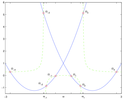
Figure 4.1: Stable. $\alpha=-1,$ $B=3$, $m_{1}=\frac{1}{4},$ and $\omega_{1}=1.$

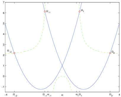
Figure 4.2: Unstable. $\alpha=-1,$ $B=3$, $m_{1}=2,$ and $\omega_{1}=1.$

5 Gyroscopic quantum oscillators

The instability results for the classical gyroscopic oscillator coupled to a heat bath can be extended directly to the quantum setting. This follows from the general quantization procedure for a classical system with quadratic Hamiltonian and gyroscopic terms. We give firstly the general analysis here as this is useful for understanding how the diagonalization procedure should be applied in the quantum case.

Consider a general classical Hamiltonian of the form

$$H(q,p)=\frac{1}{2}p^{T}M^{-1}p+q^{T}Sp+\frac{1}{2}q^{T}Kq$$ (5.1)

where $q,p$ are the $n$-dimensional position and momentum vectors respectively, and $M,S,K$ are constant $n\times n$ matrices with $M,K$ symmetric and $S$ skew-symmetric. For

$$J=\begin{bmatrix}0&I\\ -I&0\end{bmatrix}$$ (5.2)

where $I$ is the $n\times n$ identity matrix, the Hamiltonian equations of motion are given by

$$\frac{d}{dt}\begin{bmatrix}q\\ p\end{bmatrix}=J\nabla H=\begin{bmatrix}-Sq+M^{-1}p\\ -Sp-Kq\end{bmatrix}\,.$$ (5.3)

Now consider the quantization of the above system. The Heisenberg equations of motion are given by

$$i\hbar\dot{q} =[q,H]$$

$$i\hbar\dot{p} =[p,H]$$ (5.4)

where $q_{i},p_{i}$ obey the standard commutation relations. This gives

$$i\hbar\frac{d}{dt}\begin{bmatrix}q\\ p\end{bmatrix}=i\begin{bmatrix}-Sq+M^{-1}p\\ -Sp-Kq\end{bmatrix}\,.$$ (5.5)

just as in the classical setting as an easy computation shows.

The point is that the eigenvalue computation for the equations of motion in the classical setting is precisely equivalent to that for the Heisenberg equations of motion. Thus for the oscillator coupled to the heat bath the numerical computation in the classical case gives us the correct eigenvalue information for the quantum case also and we can deduce qualitative behavior as for the single gyroscopic oscillator in the previous section. Thus, for sufficiently large coupling, we observe unbound states even when the uncoupled gyroscopic oscillator exhibits bound states.

One also observes that diagonalizing the Heisenberg equations of motion is in fact equivalent to diagonalizing the Hamiltonian.

2-D gyroscopic quantum oscillator

The quantization of the uncoupled gyroscopic system illustrates that the stability analysis of the quantum system is analogous to the classical normal mode calculation. However there are some subtleties in the interpretation of the stability analysis and for this reason we consider in detail the spectral analysis of an uncoupled quantum gyroscopic systems. By the analysis of the previous section similar considerations apply to the full system of the oscillator coupled to the heat bath. We follow the Dirac formalism as described in [Messiah2] for example.

Analogously to the classical coupled oscillators, we define the quantum Hamiltonian $H$ for an oscillator in a magnetic field of strength $B$ and isotropic potential,

$$H = \frac{1}{2}(p_{x}^{2}+p_{y}^{2})+\frac{1}{2}(\frac{B^{2}}{4}+\alpha)(x^{2}+y^{2})$$

$$+\frac{B}{2}(p_{x}y-p_{y}x).$$

For a quantized gyroscopically stable oscillator, we use a standard change of coordinates to write the Hamiltonian in terms of normal modes:

$$A\pm = \sqrt{\frac{\omega_{0}}{4\hbar}}(x\mp iy)+\sqrt{\frac{1}{4\hbar\omega_{0}}}(ip_{x}\pm p_{y})$$

$$A_{\pm}^{\dagger} = \sqrt{\frac{\omega_{0}}{4\hbar}}(x\pm iy)-\sqrt{\frac{1}{4\hbar\omega_{0}}}(ip_{x}\mp p_{y}),$$

where $\omega_{0}=\sqrt{|\frac{B^{2}}{4}+\alpha|}$ and properties that $[A_{r},A_{s}]=[A_{r}^{\dagger},A_{s}^{\dagger}]=0$ and $[A_{r},A_{s}^{\dagger}]=\delta_{rs}$ for $r,s\in\{+,-\}.$ In the new coordinates, we have

$$H = \hbar(\omega_{0}-\frac{B}{2})(A_{+}^{\dagger}A_{+}+\frac{1}{2})+$$

$$\hbar(\omega_{0}+\frac{B}{2})(A_{-}^{\dagger}A_{-}+\frac{1}{2})\,.$$

We verify that the new frequencies $\omega_{0}\pm\frac{B}{2}$ are exactly the classical frequencies from the normal mode calculation. In the Heisenberg picture, we have

$$i\hbar\dot{A}^{\dagger}_{\pm} = [A^{\dagger}_{\pm},H]=-\hbar(\omega_{0}\mp\frac{B}{2})A^{\dagger}_{\pm}$$

$$A^{\dagger}_{\pm} = e^{i(\omega_{0}\mp\frac{B}{2})t}A^{\dagger}_{\pm}(t=0).$$

The eigenvalues of the Hamiltonian, $E_{n_{1},n_{2}}$ are

$$E_{n_{1},n_{2}}=\hbar\omega_{0}(n_{1}+n_{2}+1)+\hbar\frac{B}{2}(n_{1}-n_{2}),$$

where $n_{1},n_{2}\in\{0,1,2,\cdots\}.$ In the case of gyroscopic stability, we have $\frac{B}{2}>\omega_{0},$ and the energy spectrum is indefinite and unbounded above and below. In the case of pure stability ($\alpha>0$), we have $\frac{B}{2}<\omega_{0},$ and the energy spectrum in positive definite.

In the case of a quantized unstable gyroscopic oscillator, ($\frac{B}{2}+\alpha<0$), it can be shown there are no bound eigenstates.

Similarly in the case of a quantum oscillator coupled to a finite heat bath we can use the change of variables in equation (5.5) to compute the characteristic frequencies, thus reducing the coupled problem to a system of independent quantum oscillators. Thus the spectrum of the Hamiltonian of the coupled quantum system is positive if and only if the classical system is strongly stable; the spectrum is discrete with both positive and negative eigenvalues if and only if the classical system is gyroscopically stable; and finally, we have unbounded eigenfunctions if and only if the classical system in unstable.

6 Conclusions

Often one models dissipation or friction by coupling a mechanical system to a thermal reservoir. We have modeled the thermal reservoir as a collection of oscillators coupled to the mechanical system. If the reservoir is sufficiently massive, then the coupling may induce instability in the mechanical system. Equivalently, if the reservoir contains sufficiently low frequencies, then similar instabilities may arise.

Unlike other models of dissipation (i.e. Rayleigh), the conservative nature of the thermal reservoir allows us to naturally extend our results to the quantum setting. We interpret stability in the quantum setting as corresponding to bound eigenstates. A gyroscopically, stabilized, quantum Chetaev system exhibits this stability while having an unbounded spectrum.