Frenet algorithm for simulations of fluctuating continuous elastic filaments

Abstract

We present a new algorithm for generating the equilibrium configurations of fluctuating continuous elastic filaments, based on a combination of statistical mechanics and differential geometry. We use this to calculate the distribution function of the end-to-end distance of filaments with nonvanishing spontaneous curvature and show that for small twist and large bending rigidities, there is an intermediate temperature range in which the filament becomes nearly completely stretched. We show that volume interactions can be incorporated into our algorithm, demonstrating this through the calculation of the effect of excluded volume on the end-to-end distance of the filament.

Theories and computer simulations of polymers are based on the notion that a macromolecule can be modeled as a collection of points with positions $\left\{\mathbf{r}_{i}\right\}$ that represent either “real” chemically bonded monomers interacting through semi-empirical potentials (e.g., in Molecular Dynamics simulationsDennis ), or statistically independent segments connected by elastic springs or subject to constraints (in Monte Carlo simulationsBinder ). In the latter case, the elastic energy is usually assumed to be of entropic originFlory $E_{el}=\left(K/2\right)\sum_{i}(\mathbf{r}_{i}-\mathbf{r}_{i-1})^{2},$ where $K=k_{B}T/aL$ is the spring constant, $k_{B}$ the Boltzmann constant, $T$ the temperature, $L$ the polymer length and $a$ the monomer size. In polymer physics one often employs the continuum version of this theory, the so-called Gaussian chain (GC) model, in which the monomer label is replaced by a continuous contour parameter $s$, $\mathbf{r}_{i}\rightarrow$ $\mathbf{r}(s)$ and $E_{GC}=$ $\left(K^{\prime}/2\right)\int_{0}^{L}ds\left(d\mathbf{r/}ds\right)^{2}$ ($K^{\prime}$ is a constant). Alternatively, one can use the worm-like chain (WLC) model in which the energy penalty for stretching of elastic springs is replaced by bending elasticity, $E_{WLC}=\left(k_{B}Tl_{p}/2\right)\int_{0}^{L}ds\left(d^{2}\mathbf{r/}ds^{2}\right)^{2}$ where $l_{p}$ is the bending persistence length. At first sight it appears that in taking the continuum limit we pass from a description of a polymer as a collection of points to one in which it is described as a line. However, any geometrical line in 3d space must obey the Pythagorean theorem, $\left|d\mathbf{r(}s)/ds\right|=1$, a condition that can not be imposed in the framework of the GC model (it would make $E_{GC}$ a conformation-independent constant). This is consistent with the observation that the statistical properties of the GC model are identical to a those of a random walk and therefore the conformation of a polymer in this model is a fractal, with fractal dimension 2 (recall that the fractal dimension of a line is the same as its geometric dimension, 1). Although the above constraint is consistent with $E_{WLC}$, the resulting nonlinear theory appears to be intractable. Nevertheless, it was shown that the statistical mechanics of this model can be worked out using the analogy between the WLC and a quantum top, and the results were successfully applied to model the stretching of DNA moleculesMS94 .

Recently, we analyzed the statistical mechanics of the generalized WLC model that describes the linear elasticity of ribbons, with elastic energyHelix

$$E_{el}=\dfrac{1}{2}\sum_{k=1}^{3}b_{k}\int_{0}^{L}ds\left(\omega_{k}-\omega_{k0}\right)^{2},$$ (1)

where the coefficients $b_{1}$ and $b_{2}$ are associated with the bending rigidities with respect to the two principal axes of inertia of the cross section (they differ if the cross section is not circular), and $b_{3}$ represents twist rigidity. In this paper we will treat $\left\{b_{i}\right\}$ as given material parameters of the filament. The functions $\left\{\omega_{k}(s)\right\}$ and $\left\{\omega_{k0}(s)\right\}$ are related to the generalized curvatures and torsions in the deformed and the stress-free states of the filament, respectively. These parameters completely determine the three dimensional conformation of the centerline and the twist of the cross-section about this centerline, through the generalized Frenet equations

$$\dfrac{d\mathbf{t}_{i}(s)}{ds}=-\sum_{j,k}\varepsilon_{ijk}\omega_{j}(s)\mathbf{t}_{k}(s).$$ (2)

Here $\mathbf{t}_{3}$ is the unit tangent to the centerline and the unit vectors $\mathbf{t}_{1}$ and $\mathbf{t}_{2}$ are oriented along the principal axes of the cross section ($\varepsilon_{ijk}$ is the antisymmetric tensor). Note that since these equations describe a pure rotation of the triad $\left\{\mathbf{t}_{i}(s)\right\}$ as one moves along the contour of the filament, the constraint $\left|\mathbf{t}_{3}\right|=\left|d\mathbf{r(}s)/ds\right|=1$ is automatically satisfied in this intrinsic coordinate description.

Since the energy is a quadratic form in the deviations $\delta\omega_{k}=\omega_{k}-\omega_{k0}$ of the curvature and torsion parameters from their values in the stress free state (Eq. (1) is valid as long as the characteristic length scale of the deformation is larger than the diameter of the filamentLove ), the distribution of $\delta\omega_{k}$ is Gaussian, with zero mean and second moments given byHelix

$$\left\langle\delta\omega_{i}(s)\delta\omega_{j}(s^{\prime})\right\rangle=\dfrac{k_{B}T}{b_{i}}\delta_{ij}\delta(s-s^{\prime}).$$ (3)

Using the above expression we showed that all the two-point correlation functions $\left\langle\mathbf{t}_{i}(s)\cdot\mathbf{t}_{j}(s^{\prime})\right\rangle$ can be calculated by solving a simple linear differential equation with $s$-dependent coefficients, for arbitrary parameters of the stress free state $\left\{\omega_{k0}\right\}$ and rigidity parameters $\left\{b_{k}\right\}$. However, since the distribution functions of the various fluctuating quantities (e.g., the end-to-end distance $R$) are non-Gaussian, knowledge of the second moments does not determine the distributions and therefore, the complete determination of the statistical properties of fluctuating ribbons requires more powerful analytical or numerical methods. In this paper we present an efficient algorithm for the simulation of fluctuating elastic ribbons and use it to study the effects of spontaneous curvature and twist rigidity on the spatial conformations of fluctuating ribbons. To the best of our knowledge this is the first direct simulation of continuous lines (other simulations of the WLC model and its extensions represent the filament as a collection of points Frey ; Kremer ; Maggs ).

Examination of Eq. (3) shows that the decoupling of the “noises” $\left\{\delta\omega_{k}\right\}$ in the intrinsic coordinate representation permits an efficient numerical generation of independent samples drawn from the exact canonical distribution. The Gaussian distribution of the $\delta\omega_{k}$ means that each $\delta\omega_{k}(s)$ can be directly generated as a string of independent random numbers drawn from a distribution symmetric about the origin with width $\sqrt{k_{B}T/b_{k}ds},$ where $ds$ is the discretization step length. Note that the discretization of the continuous filament (choice of $ds$) is a computational tool only, and is very different from the case of a chain consisting of discrete mass points. We always choose $ds$ sufficiently small so that the results are insensitive to its precise value.

The remaining task is to construct the curve using the Frenet equations with $\omega_{k}(s)=\omega_{k0}(s)+\delta\omega_{k}(s)$. The Frenet equations are best integrated by stepping the basic triad $\left\{\mathbf{t}_{k}\right\}$ forward in $s$ through a suitable small rotation. In this way, the orthonormality of the triad is guaranteed to be preserved up to machine accuracy. To construct this rotation matrix, we begin with Eq. (2) and, defining the three vectors $v^{x}=(t_{1}^{x},t_{2}^{x},t_{3}^{x})$, and so forth, we can write this equation as

$$\frac{dv^{i}}{ds}=Av^{i}$$ (4)

where $A$ is an antisymmetric matrix with elements $A_{ij}=\sum_{k}\varepsilon_{ijk}\omega_{k}$. We now discretize Eq. (4) as

$$v^{i}(s+ds)=Ov^{i}(s)$$ (5)

where the orthogonal matrix $O$ is

$$O=\left(1+\frac{ds}{2}A\right)\left(1-\frac{ds}{2}A\right)^{-1}$$ (6)

In the following we present the results of simulations of distribution of the end-to-end distance for a filament of contour length $L=1$ and study its dependence on the stress free configuration $\left\{\omega_{k0}\right\},$ rigidity parameters $\left\{b_{k}\right\}$ and temperature.

We first consider a straight filament, with $\omega_{10}=\omega_{20}=\omega_{30}=0$. In the limit $T\rightarrow 0$, the distribution $P(R)$ of the end-to-end distance, $R$, approaches a delta function peaked at $R=1$. With increasing $T,$ the peak of the distribution shifts to smaller values of $R,$ consistent with the fact that the effective persistence length scales as $l_{p}\sim b/k_{B}T$ ($b$ is a characteristic bending rigidity parameter). The behavior of the width of the distribution is more interesting. Initially (in the range $l_{p}\gg 1$) the distribution broadens with $T$ and then narrows down again as the Gaussian chain limit $\left\langle\mathbf{R}^{2}\right\rangle=l_{p}L\propto 1/T$ is approached for $l_{p}\ll 1$. This behavior is universal and takes place for arbitrary values of the rigidity parameters; furthermore, the form of the distribution depends only on the bending rigidities $b_{1},$ $b_{2}$ and is unaffected by the twist rigidity $b_{3}.$

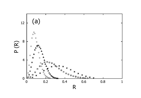
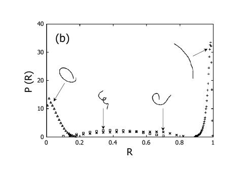
Figure 1: Plot of the distribution function $P(R)$ vs. the end-to-end to end distance $R$ for an open ring. a) $b_{1}=b_{2}=b_{3}=1$, and temperatures $T=0.1$ (circles), 1 (squares), 10 (crosses) and 100 (triangles). b) $b_{1}=b_{2}=1$, $b_{3}=10^{-4}$, and temperatures $T=10^{-5}$ (triangles), $10^{-3}$ (crosses), 0.1 (pluses) and 10 (squares). Snapshots of typical configurations corresponding to each of these temperatures are shown as inserts.

Now consider a ring, broken at a point so that the ends are free to fluctuate. Here $\omega_{10}=2\pi$, $\omega_{20}=\omega_{30}=0$. In Fig. 1a we present the distribution function $P(R)$ for the case $b_{1}=b_{2}=b_{3}=1$. As dictated by the geometry of the stress free state, $P(R)$ approaches a delta function peaked at $R=0$ in the limit $T\rightarrow 0.$ At higher temperatures, fluctuations increase $R$, the distribution broadens and its peak moves out to higher values of $R$ of the order of the diameter of the ring ($1/\pi$). At yet higher $T$ the decrease of the persistence length with increasing temperature takes over, the distribution narrows and its peak moves to smaller values of $R$.

In Fig. 1b we present the case of the broken ring now at small twist rigidity ($b_{3}\ll b_{1},b_{2}$). While the low temperature behavior is similar to that in Fig 1a, nearly full stretching accompanied by a dramatic narrowing of the distribution of the end-to-end distance is observed at intermediate temperatures for which $a_{1}/L=a_{2}/L>1,$ $a_{3}/L\ll 1$ (we define the bare persistence lengths, $\left\{a_{i}\right\}=\left\{b_{i}/k_{B}T\right\}$). This striking observation is supported by analytical results for the mean square end-to-end distanceHelix $\left\langle\mathbf{R}^{2}\right\rangle=2\int_{0}^{L}ds\int_{0}^{s}ds^{\prime}\left[e^{-\mathbf{\Lambda}\left(s-s^{\prime}\right)}\right]_{33},$ where the elements of the matrix $\mathbf{\Lambda}$ are $\Lambda_{ik}=\left(k_{B}T/2\right)\left[\sum_{j}1/b_{j}-1/b_{i}\right]\delta_{ik}+\sum_{l}\varepsilon_{ikl}\omega_{l0}.$ An exact expression for $\left\langle\mathbf{R}^{2}\right\rangle$ in terms of the parameters $\left\{b_{k}\right\}$ was derived by diagonalizing the matrix $\mathbf{\Lambda}$ and is compared against our simulation results in Fig. 2. We would like to emphasize that the nearly complete stretching of the filament is a finite $L$ effect and that the renormalized persistence length defined by $l_{p}=\lim_{L\rightarrow\infty}\left\langle\mathbf{R}^{2}\right\rangle/L,$ does not diverge in the limit of vanishing twist rigidity.

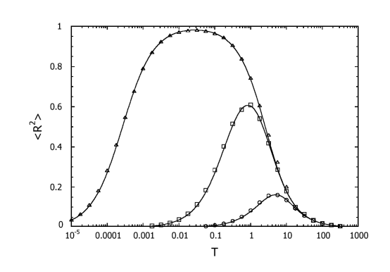
Figure 2: Simulation results for the mean square end-to-end distance $\left\langle R^{2}\right\rangle$ vs. temperature $T$ for an open ring, with $b_{1}=b_{2}=1$ and $b_{3}=1$ (circles), $b_{3}=10^{-2}$ (squares) and $b_{3}=10^{-5}$ (triangles). The results of the analytical calculations are shown as solid lines.

The observation of nearly complete stretching of the filament is at first sight counterintuitive, given that at these temperatures, its bending persistence length is larger than its contour length, and so thermal fluctuations can not significantly change the curvature from its finite spontaneous value ($\omega_{10}=2\pi$), let alone cause it to vanish. The resolution of this paradox is that our intuition that a circle can not be continuously deformed into a line, at fixed curvature, is wrong. Any 3d curve can be described by its curvature $\omega_{1}$ and torsion $\omega_{3}$ (if we replace the filament by a geometrical line, we should setHelix $\omega_{2}=0$). Keeping the curvature fixed and increasing the torsion (assumed to be constant along the filament), one goes from a circle of radius $\omega_{1}^{-1}$ to an increasingly stretched helix, with radius $\omega_{1}/\left(\omega_{1}^{2}+\omega_{3}^{2}\right)\rightarrow 0$ and end-to-end separation approaching that of a straight line. This indeed takes place in our case since Eq. (3) gives $\left\langle\omega_{3}^{2}\right\rangle=k_{B}T/(b_{3}ds)$ so that thermal fluctuations of the torsion $\omega_{3}$ are large in the limit of small twist rigidity. Since, under conditions of nearly complete stretching, the distribution of the end-to-end distance is extremely narrow (see Fig. 1b), mean field considerations apply and we can describe the filament as an object with length $L=1,$ curvature $\omega_{1}=2\pi$ and torsion $\left\langle\omega_{3}^{2}\right\rangle^{1/2}=\pm\sqrt{k_{B}T/(b_{3}ds)}.$ For high temperature and small twist rigidity, $|\left\langle\omega_{3}^{2}\right\rangle^{1/2}|\gg\omega_{10}$, this object is a nearly straight helix that oscillates between left-hand and right-hand forms as one moves along its axis (in this limit the change of sign of torsion changes the sense of helical rotation but does not affect the direction of the axis about which the helix rotates), with typical radius of helical turn $2\pi b_{3}ds/(k_{B}T)$ that is much smaller than its pitch $2\pi\sqrt{b_{3}ds/(k_{B}T)}.$ Since in this limit the pitch approaches the period of the helix, we conclude that the helical filament is nearly completely stretched. At yet higher temperatures, the bending persistence length becomes shorter than the length of the filament, the helical structure “melts”, and one recovers the Gaussian chain behavior characteristic of flexible polymers.

In order to demonstrate that volume interactions between parts of the filament can be readily incorporated into our algorithm, we calculated the Flory exponent $\nu$ defined by the relation, $\left\langle\mathbf{R}^{2}\right\rangle\sim L^{2\nu}$. We inserted $50$ equally spaced interaction sites per unit length into the filament ($50L$ sites in total) and allowed only configurations in which the spatial distance between any two of these sites exceeded $0.01.$ For each value of $L$ we generated $1000$ allowed configurations and calculated the average value of $\mathbf{R}^{2}$. We first checked that when all configurations were allowed (no excluded volume), we obtain the Gaussian random walk result, $\nu_{0}\approx 0.51.$ In the presence of excluded volume, the best fit to the simulation (Fig. 3), yields $\nu_{SAW}\approx 0.59,$ in excellent agreement with the Flory exponent of $3/5$ for self-avoiding polymers in 3dFlory .

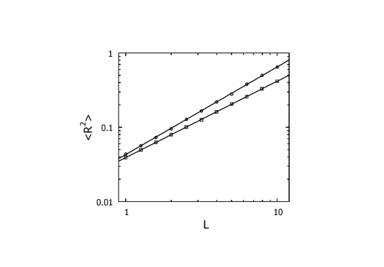
Figure 3: Simulation results for the mean square end-to-end distance $\left\langle R^{2}\right\rangle$ vs. the contour length $L$ for a linear filament, with (circles) and without (squares) excluded volume. The solid lines give the least square fit to the data. The parameters are $b_{1}=b_{2}=b_{3}=0.02$, and $T=1.$

In closing, we would like to comment on possible ramifications of this work. The methods presented in this work are ideally suited to investigate polymers with spontaneous curvature such as double stranded DNATTH87 , and synthetic molecules with bent coresLink . As far as equilibrium properties are concerned, our algorithm is computationally far superior to standard Monte-Carlo methods in that each realization of the filament is completely independent. Because sequence dependence can be readily incorporated into the present theory through the dependence of the spontaneous curvature and torsion parameters $\left\{\omega_{k0}(s)\right\}$ on the contour position $s,$ and because the method is easily extendible to incorporate excluded volume, electrostatic and other self-interaction effects, the Frenet algorithm has the potential of becoming an important new tool for computer simulations of equilibrium properties of complex biopolymers such as DNA, RNA and proteins.

- (1) D.C. Rapaport, The Art of Molecular Dynamics Simulation (Cambridge University Press, Cambridge, 1995).
- (2) D.P. Landau and K. Binder, A Guide to Monte Carlo Simulations in Statistical Physics (Cambridge, Cambridge, 2000).
- (3) P.J. Flory, Principles of Polymer Science (Cornell University Press, Ithaca, 1953).
- (4) J.F. Marko and E.D. Siggia, Macromolecules 27, 981 (1994); C. Bustamante, J.F. Marko, E.D. Siggia and S.B. Smith, Science 265, 1599 (1994).
- (5) S. Panyukov and Y. Rabin, Phys. Rev. Lett. 85, 2404 (2000); Phys. Rev. E62, 7135 (2000).
- (6) A.E.H. Love, A Treatise on the Mathematical Theory of Elasticity (Dover, New York, 1944).
- (7) J. Wilhelm and E. Frey, Phys. Rev. Lett. 77, 2581 (1996).
- (8) T.B. Liverpool, R. Golestanian, and K. Kremer, Phys. Rev. Lett. 80, 405 (1998).
- (9) R. Everaers, F. Julicher, A. Ajdari and A.C. Maggs, Phys. Rev. Lett. 82, 3717 (1999).
- (10) E.N. Trifonov, R.K.-Z. Tan and S.C. Harvey, in DNA Bending and Curvature, W.K. Olson, M.H. Sarma and M. Sundaralingam eds. (Adenine Press, Schenectady, 1987); J. Bednar et al, J. Mol. Biol. 254, 579 (1995).
- (11) D.R. Link et al., Science 278, 1924 (1997).