Measuring Anti-Correlations in the Nordic Electricity Spot Market by Wavelets

Abstract

We consider the Nordic electricity spot market from mid 1992 to the end of year 2000. This market is found to be well approximated by an anti-persistent self-affine (mean-reverting) walk. It is characterized by a Hurst exponent of $H\simeq 0.41$ over three orders of magnitude in time ranging from days to years. We argue that in order to see such a good scaling behavior, and to locate cross-overs, it is crucial that an analyzing technique is used that decouples scales. This is in our case achieved by utilizing a (multi-scale) wavelet approach. The shortcomings of methods that do not decouple scales are illustrated by applying, to the same data set, the classic $R/S$- and Fourier techniques, for which scaling regimes and/or positions of cross-overs are hard to define.

1 Introduction

Over the last ten years, or so, dramatic changes have occurred, and are still on-going, in the energy sectors of the world. What used to be well established monopolies in many countries and regions, were deregulated in such a way that consumers could buy their electricity from other sources then their local provider. These changes opened up for competition on the price of electric energy. Energy exchanges were created, as a result, as places where such organized transactions could take place.

One of the first electricity markets in the world to be deregulated was the Norwegian, that was fully deregulated by 1992. The same year a Norwegian commodity exchange for electric power was established. Here one could trade short and long term electricity contracts in addition to contracts for next-day ($24\,h$) or immediate physical delivery. This market place, which now also includes the other Nordic countries, is today known as NordPool — the Nordic Power Exchange [1].

The next-day electricity market, i.e., where contracts for $24\,h$ delivery are traded, is known as the spot market. This market, administrated by NordPool, is open $24$ hours a day $7$ days a week all year around, and the (spot) price is fixed for each hour separately. In this market, participants (i.e. the buyers and sellers) tell the market administrator (NordPool) how much, and to what price and at what time they want to sell or buy a given amount of electric power. From these bid and ask data the administrator creates a market cross which sets the spot price for that particular hour. The market cross is obtained by forming the cumulative volume histograms, $V_{s}(p)$ and $V_{b}(p)$, that give respectively the total amount of electric energy that sellers (buyers) want to sell (buy) at a price higher (lower) then $p$. The spot price, $S$, is then defined as the price at which $V_{s}(S)=V_{b}(S)$ (if such a point exists). Thus, the spot price is set such that the total volume of sold and bought electric power is balanced. All sellers asking a price $p\leq S$, as well as all buyers willing to pay $p\geq S$ will get a transaction at the spot price for that particular hour. In all other cases no transactions will take place. If no market cross can be defined from the bid and ask data, no transactions will take place and the spot price for that particular hour remains unset.

Recently, it has been suggested that the electricity spot price process is a so-called mean-reverting process [2, 3]. Here, the degree of mean-reversion was quantified for the Californian spot power market by measuring its Hurst or roughness exponent by the $R/S$-analysis [4, 5]. However, in order to perform this analysis, Weron and Przybyłowicz [2] had to consider the daily average returns instead of the hourly returns. This is due to a shortcoming of the $R/S$-method when analysing multi-scale time series as we will see explicitly in the discuss below.

In this paper, however, we suggest to use another technique — a wavelet based analyzing technique that does not suffer from this shortcoming. The method is demonstrate on data from NordPool — the oldest multi-national power exchange in the world. It is found that the Nordic electricity power market is anti-persistent (mean-reverting), and the (Hurst) exponent characterizing the market is found to be $H=0.41\pm 0.02$ for time scales ranging from days to years, where the error indicated is the regression error.

2 The data set

The data we analyzed are the official NordPool spot price data (system price) [1] collected over the period from May 4, 1992 to December 31, 2000. They cover more then eight and a half years of hourly logged data, which corresponds to somewhat more then $75\,000$ data points for the whole data set.

The analyzed data set is depicted in Fig. 1. From this figure one easily observes the daily and seasonal trends that are characteristic of the spot price. Such trends are most likely attributed to the consumption patterns of the market. For instance, in the Californian electricity spot market the high price season is the summer season [2] while for the Nordic power market it is the winter. These high price seasons coincide with the peaks in consumption which are different due to the climatic differences between the Nordic countries and California.

Even though we are talking about the Nordic power market, it should be realized that during the period from 1992 to 2000 the market has changed its structure when it comes to participating countries. In the beginning, the market was a pure Norwegian market, because Norway was the first Nordic country to deregulate its power sector. Roughly five years later, during late 1995 and early 1996, Sweden and Finland deregulated their electricity markets, and became members of what today is the NordPool system. So, first at this point in time it is fair to talk about a real Nordic Power exchange. Finally, last year also Denmark joined in, while there for the moment seems to be no indication that Island, as the last remaining Nordic country, will do the same.

3 Self-affine processes and mean-reversion

A time-dependent function $p(t)$ is said to be self-affine if fluctuations on different time scales can be rescaled so that the original signal $p(t)$ is statistical equivalent to the rescaled version $\lambda^{-H}p(\lambda t)$ for any positive number $\lambda$ [5], i.e.,

$$p(t)\simeq\lambda^{-H}p(\lambda t),$$ (1)

where $\simeq$ is used to denote statistical equality. Here $H$ is the so-called Hurst (or roughness) exponent [5], an exponent which quantifies the degree of correlation — positive or negative — in the increments $\Delta p(t)=p(t)-p(0)$. It can be shown that for a process satisfying Eq. (1) the correlation function $C(t)$ between future, $\Delta p(t)$, and past, $\Delta p(-t)$, increments is given by [5]

$$C(t)=\frac{\left<-\Delta p(-t)\Delta p(t)\right>}{\left<\left[\Delta p(t)\right]^{2}\right>}=2^{2H-1}-1.$$ (2)

From the above expression one should notice that $C(t)$ is time-independent, and that for a Brownian motion ($H=1/2$) past and future increments are uncorrelated ($C(t)=0$) as is well-known. However, if $H>1/2$ the increments are positively correlated ($C(t)>0$) and for $H<1/2$ they are negatively correlated ($C(t)<0$). In the former case we say that the process $p(t)$ is persistent while in the latter one talks about an anti-persistent (or anti-correlated) process. In the economics literature anti-persistency is known under the name of mean-reversion.

4 The Average Wavelet Coefficient Method

The Average Wavelet Coefficient Method (AWC) [6, 7] is a method that utilizes the wavelet transform [8, 9] in order to measure the temporal self-affine correlations of a time series, i.e., a method for measuring its Hurst exponent $H$. This is done by transforming the time series, $p(t)$, into the wavelet-domain, ${\mathcal{W}}[p](a,b)$, where $a$ and $b$ represent a scale and location parameter, respectively [8, 9]. The AWC-method consists of, for a given scale $a$, to find a representative wavelet “energy” or amplitude for that particular scale, and to study its scaling. This can, for instance, be done by taking the arithmetic average of $|{\mathcal{W}}[p](a,b)|$ over all location parameters $b$ corresponding to one and the same scale $a$. Thus, one can construct from the wavelet transform of $p(t)$, the AWC-spectrum $W[p](a)$ (to be defined below) so that it will only depend on the scale $a$. If $p(t)$ is a self-affine process characterized by an exponent $H$, this spectrum should scale as [7, 10]

$$W[p](a)=\left<\left|{\mathcal{W}}(a,b)\right|\right>_{b}\sim a^{H+1/2}.$$ (3)

Thus, if we plot $W[p](a)$ vs. scale $a$ in a log-log plot, the slope should be $H+1/2$ if the signal is self-affine. We note that this method is a multi-scale method in the sense that the behavior at different scales does not influence each other in any significant way, i.e., the method decouples scales as we will see exemplified below. This decoupling of scales comes about due to the wavelets being orthogonal [8, 9].

5 Numerical results

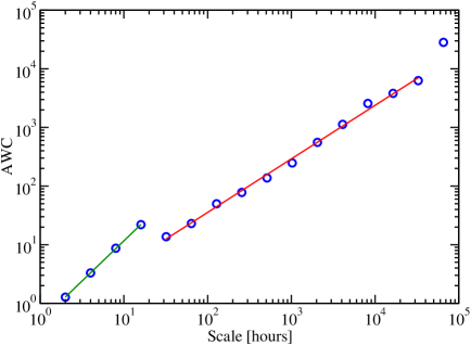
Figure 2: The AWC spectrum, $W[p](a)$ vs. scale $a$, for the hourly Nordic electricity spot data presented in Fig. 1. A cross-over at $a_{\times}\sim 24\,h$ is easily observed in the $W[p](a)$-spectrum. The scaling region $a>a_{\times}$ corresponds to a Hurst exponent of $H=0.41\pm 0.02$ where the uncertainty is a pure regression error. The slope of the spectrum for $a<a_{\times}$ seems to indicate a persistent behavior ($H>0.5$). The wavelet used in obtaining these results was of the Daubechies type (DAUB24).

In Fig. 2 we present the AWC-spectrum, $W[p](a)$, for the Nordic electricity spot price time series depicted in Fig. 1. Probably the most striking feature of this spectrum is the nice and large scaling regime for scales bigger then one day ($a>24\,h$). Its size extends over three orders of magnitude in time ranging from days to several years. The Hurst exponent characterizing this scaling region is found by a regression fit to the functional form given by Eq. (3). Such a fit, indicated by a solid line in Fig. 2, results in a Hurst exponent of

$$H=0.41\pm 0.02,$$ (4)

where the error bar is a pure regression error. This value for the Hurst exponent means that the spot prices process is anti-persistent (anti-correlated) or equivalently mean-reverting. Another way of saying the same is that a price drop, say, in the past is more likely in the future to be followed by an increase in the price then by another price drop.

Due to the entrance of Sweden and Finland into the spot market in the years of 1995 and 1996, it is interesting to see if this did affect the statistical properties of the spot market in any significant way. To study this, we have compared the Hurst exponents for the two periods 1992–1995 and 1996–2000. We found that within the error bars, the Hurst exponents for these two periods could not be distinguished, even though the numerical value of the exponent was decreased somewhat from the first to the second period.

It is also interesting to notice that the value measured for the Hurst exponent of the Nordic spot market, Eq. (4), is more or less the same as the one reported earlier for the Californian market. For this latter market Weron and Przybyłowicz [2] found $H=0.42-0.43$. For the moment it is too early to say if the reasons for these values being so similar is just a coincidence or there exists more fundamental reasons for it.

The size, and quality, of the scaling regime for $a>24\,h$ we find somewhat surprising. First, the data contains of both daily as well as seasonal trends, non of which have been removed from the analyzed data set. Since we are using an analyzing method that decouples scales, the daily trend should not influence the (day-to-day) scales considered. However, the seasonal trends, typically with highest prices during winter time, could in principle affect the scaling regime. This trend seems, however, to have little or no effect on the spectrum in practice [11]. Hence, we can for instance by studying the week-to-week price changes get information about the year-to-year price changes simply by a rescaling of the problem according to Eq. (1) with the value for the Hurst exponent given by Eq. (4) — i.e. we have scale invariance!

We just saw that the Nordic electricity spot prices on a time scale bigger then one day is well approximated by an anti-persistent self-affine walk. Such anti-correlations are rather atypical for financial time series. For instance for liquid stock indices one typically finds them to be uncorrelated after a rather short time period [12, 13]. Anything else would give rise to arbitrage opportunities due to the correlated (or anti-correlated) increments [14]. By exploiting these correlations by for instance adapting an investment strategy that takes them into consideration, they will most likely vanish. That this apparently does not happen for the electricity spot market we believe is related to the fact that electricity, for the moment, can not be stored efficiently. Even if we knew for sure that the spot price would increase tomorrow, we could not buy electricity today and sell it with profit tomorrow simply because we do not have a way of storing it in the mean time in an economical way. Therefore, there seems at present to be no profit opportunity created by the anti-correlation in the spot price increments. However, if technological advances in the future will allow for an efficient storage of electricity (at moderate cost), the situation will probably be quite different. Then profit opportunities will exist, and we expect anti-correlations to disappear for time scales where efficient storage of electricity is feasible.

Another striking feature of the AWC-spectrum shown in Fig. 2 is the sharp cross-over taking place at roughly one day, i.e., at a scale $a=a_{\times}=24\,h$. At scales bigger then this, we just saw that we had anti-correlation. However, at smaller scales, it seems more reasonable to assume that the price increments are correlated. If we temporary assume a scaling regime for scales $a<a_{\times}$ (that we will not insist on), one from a regression fit obtains $H=0.87\pm 0.02$. Hence, it should be clear that the spot price time series behaves differently on an intra-day scale then on a day-to-day scale (or bigger). In fact, such an observation can be done directly from Fig. 1 by visual inspection.

Finally, we would like to give some explicit examples showing the need of an analyzing method that decouples scales when handling multi-scale time series. This we will do by applying the classic rescaled-range (or $R/S$) and the popular Fourier analyzing technique to our data set [5]. Notice that none of these two methods do decouple the scales involved. In the $R/S$-analysis, one calculates the range, $R(w)$, defined as the average vertical distance between the maximum and minimum point of the cumulative signal calculated over a window of size $w$, divided by the (average) standard deviation, $S(w)$, of the original signal taken over the same window size. It can be shown that the ratio $R/S$ of a self-affine series should scale according to $w^{H}$. The Fourier method, on the other hand, is performed by calculating the power spectrum of the time-series, $P(\omega)$, where $\omega=2\pi/\nu$ denotes the angular frequency with $\nu$ being the frequency. For a self-affine time series, this quantity should scale as $P(\omega)\sim\omega^{-2H-1}$. The interested reader is referred to Ref. [5] for a detailed introduction to both these two methods.

The result of a $R/S$ analysis of the NordPool spot data is presented in Fig. 3. We observe that only for a small window size (or scale) corresponding to a day or less, do we have a signature of a scaling regime, but, as above, it is too small to be called so. This region is what corresponds to what we found for the intra-day price increments ($a<24\,h$) in our wavelet analysis, and the corresponding exponents obtained from the two methods are also found to be similar. However, when we focus at bigger scales, we notice, according to the $R/S$ technique, that there is no scaling region since the $R/S$-function is curved in this region. From the wavelet analysis, however, we have seen that there should be a rather robust scaling regime for $a>a_{\times}$. The solid line in Fig. 3 indicates the slope corresponding to the Hurst exponent previously measured by the wavelet technique and given by Eq. (4). Such a regime can hardly be defined for the $R/S$-function in this region. The reason why the scaling regime is not found by the rescaled-range method is that the calculation of the $R/S$-function for large window sizes is influenced substantially by smaller window sizes. This is particularly seen at the cross-over; Just above the cross-over, the rescaled-range signal will be dominate by the behavior below the cross-over, resulting in a smear-out in this region. One observes from Fig. 3 that this cross-over transition hampers the scaling behavior for several orders of magnitude in scale after the cross-over. In fact for this particular case, no scaling is possible to observe at all for scales ranging from the cross-over and up to the maximum scale studied. Thus, we may conclude that the $R/S$-method is not well suited for analyzing time-series that possess multiple scale behavior. This is the reason why Weron and Przybyłowicz [2] analyzed, by the rescaled-range method, the daily averaged returns instead of the hourly price increments themselves. We have also checked that analyzing the daily averaged returns of our data set by the $R/S$-method produces a scaling regime of a Hurst exponent consistent with the one previously found by the wavelet technique.

In the inset to Fig. 4 we present the power spectrum $P(\omega)$ vs. (angular) frequency $\omega$ for our time series. It is observed, as is a rather typical case, that the raw power spectrum is somewhat noisy, and that the cross-over that we know should be there is not so easy to locate. In order to reduce the noise level, it is rather common to use a so-called log-binning technique. This amounts to using a gliding window of a size that increases logarithmically with frequency, and to take the average of the power spectrum within this window. Strictly speaking, this is not a rigorous approach, but if the window size is not too large it does not seem to have any practical consequence for the estimated scaling exponents. The results of such a procedure is shown in the main part of Fig. 4, and one observes a dramatic reduction in the noise. The solid line in this figure represents the $\omega^{-2H-1}$ behavior where for the Hurst exponent we have used that of Eq. (4) (the wavelet result). For the Fourier method, in contrast to the rescaled-range method, there is a reasonable agreement with the wavelet method when the hourly price data are used. If we measure the Hurst exponent from the (log-binned) power spectrum we find $H=0.42\pm 0.04$ that should be compared with the value $H=0.41\pm 0.02$ that we obtained by the AWC-method. As before, the error bars are pure regression errors, and the real error is of course somewhat bigger.

Notice, however, that even after log-binning the cross-over in the power spectrum expected to be located at $\omega_{\times}=2\pi/a_{\times}=0.26\,h^{-1}$, is not that sharp or well pronounced, even though there seems to be some indication of it. The two peaks in the power spectrum at approximately $\omega\simeq 0.5\,h^{-1}$ and $1\,h^{-1}$, corresponding in scale ($a=2\pi/\omega$) to $a\simeq 12\,h$ and $6\,h$ respectively, are caused by the intra-day price increase due to the consumption pattern with high consumption in the morning and afternoon (see the inset to Fig. 1). This effect was not caught by the wavelet technique used in this paper. We believe that the reason for this is the use of the discrete wavelet transform which does not include the scales $6\,h$ or $12\,h$. However, such enhanced correlations, we suspect, will be caught if the continuous wavelet transform is used instead of a discrete one [15].

6 Conclusions

We have analyzed the hourly logged spot electricity prices from the Nordic electricity power market over a eight and a half years period starting in mid 1992. It is found that the spot price process is an anti-persistent self-affine walk (mean-reverting stochastic process) over at least three orders of magnitude in time ranging from days to years. Hence the increments in the spot price process are anti-correlated over the same time scales. The Hurst exponent that characterize this scaling behavior was measured by a wavelet technique and found to be $H=0.41\pm 0.02$, where the error bar is a pure regression error. We also commented on other classical methods of measuring such exponents and stressed and showed that it is important to use methods that decouple scales when multi-scale time series are being analyzed.

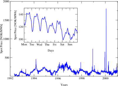
Figure 1: The hourly Nordic electricity spot prices (system price) for the period from May 4, 1992 to December 31, 2000 [1]. The total number of data points is somewhat larger then $75\,000$. The inset shows the spot prices for the first week of year 2000 staring on Monday January 3. From the inset one should observe the daily price trends.

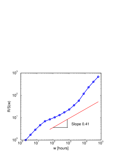
Figure 3: The $R/S$-analysis of the hourly Nordic electricity spot data presented in Fig. 1. Notice that no scaling regime can be defined for window sizes bigger then one day (see text for explanation). The solid line corresponds to $w^{H}$ with $H=0.41$ as measured by the AWC-method.

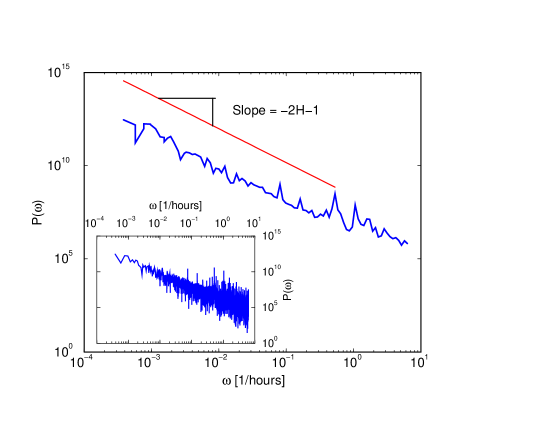
Figure 4: The Fourier-analysis of the hourly Nordic electricity spot data presented in Fig. 1. The inset shows the raw power spectrum, $P(\omega)$ vs. angular frequency $\omega$ for the spot price data. In order to reduce the noise of the raw power spectrum, we have applied the log-binning technique to it, resulting in the power spectrum shown in the main figure. The solid line of this figure corresponds to $\omega^{-2H-1}$ with the value of $H$ obtained from the AWC-technique (Eq. (4)). The pronounced cross-over seen in Fig. 2 corresponds to an angular frequency of $\omega_{\times}=2\pi/a_{\times}\sim 0.26\,h^{-1}$, but such a cross-over is not easily located in the power spectrum. A direct regression fit to the log-binned power spectrum for $\omega<\omega_{\times}$ results in $H=0.42\pm 0.04$.

References

- [1] See NordPools’s web-page : http://www.nordpool.no.
- [2] R. Weron and B. Przybyłowicz, Physica A 283, 462 (2000).
- [3] R. Weron, Physica A 285, 127 (2000).
- [4] H. E. Hurst, Trans. Am. Soc. Civil Engnr. 116, 770 (1951).
- [5] J. Feder, Fractals (Plenum Press, New York, 1988).
- [6] A. R. Mehrabi, H. Rassamdana, and M. Sahimi, Phys. Rev. E 56, 712 (1997).
- [7] I. Simonsen, A. Hansen, and O. Nes, Phys. Rev. E 58, 2779 (1998).
- [8] I. Daubechies, Ten Lectures on Wavelets (SIAM, Philadelphia, 1992).
- [9] D. B. Percival and A. T. Walden, Wavelet Methods for Time Series Analysis (Cambridge University Press, Cambridge, 2000).
- [10] Here we could also have used another norm with , but we will not consider this option here. In practice the results show little sensitivity to the choice of (for moderate values).
- [11] Technically, this comes about due to the wavelet being orthogonal to any polynomial up to a given order.
- [12] J.-P. Bouchaud and M. Potters, Theory of financial risks : from statistical physics to risk management (Cambridge University Press, Cambridge, 2000).
- [13] R. N. Mantegna and H. E. Stanley, An Introduction to Econophysics: Correlations and Complexity in Finance (Cambridge University Press, Cambridge, 2000).
- [14] I. Simonsen and K. Sneppen, Physica A 316, 561 (2002).
- [15] I. Simonsen, work in progress (unpublished).