[

Coulomb Blockade Peak Spacing Distribution: The Interplay of Temperature and Spin

Abstract

We calculate the Coulomb Blockade peak spacing distribution at finite temperature using the recently introduced “universal Hamiltonian” to describe the $e$-$e$ interactions. We show that the temperature effect is important even at $k_{B}T\!\sim\!0.1\Delta$ ($\Delta$ is the single-particle mean level spacing). This sensitivity arises because: (1) exchange reduces the minimum energy of excitation from the ground state and (2) the entropic contribution depends on the change of the spin of the quantum dot. Including the leading corrections to the universal Hamiltonian yields results in quantitative agreement with the experiments. Surprisingly, temperature appears to be the most important effect.

]

Among the unique features of quantum dots (QDs) is the possibility to control their number of electrons $N$. [1] This is done by weakly coupling a QD to source and drain leads and using a gate voltage $V_{g}$ to control its electrostatic potential. When the thermal energy $k_{B}T$ is smaller than the charging energy $E_{C}$ required to add an electron to the QD, the electron transport is blocked and $N$ is fixed. By sweeping $V_{g}$ this Coulomb Blockade (CB) effect can be overcome at the particular value $V_{g}^{N}$ where the transition $N\!\rightarrow\!N+1$ occurs. The conductance $G(V_{g})$ shows then a series of sharp peaks as a function of $V_{g}$.

At sufficiently low temperature, $k_{B}T\!\ll\!\delta$ where $\delta$ is the energy gap between the ground state (GS) and the first excited state of the QD, only the former contributes significantly to the conductance peak. In that case, the position of the CB peak is proportional to the change of the GS energy of the QD upon the addition of one electron. [1] Therefore, the CB peak spacing distribution (PSD) yields information about the many-body GS properties of the QD.

This has been the subject of experimental [2, 3, 4, 5, 6] and theoretical [7, 8, 9, 10, 11, 12, 13, 14, 15] work over the last years. One reason is that the simplest model used for the CB conductance peaks fails drastically in describing the observed PSD. It assumes a constant $e$-$e$ interaction ($E_{C}$)—hence the name constant interaction (CI) model. Recently, however, it has become clear that residual $e$-$e$ interactions (i.e., those beyond $E_{C}$) play an important role in determining the GS of the QD [7, 8, 9, 10, 11, 12, 13, 14] and therefore must be included in the description of the PSD. In particular, the addition of the average exchange interaction, [10, 11, 12] which gives the “universal Hamiltonian”, hereafter called the constant exchange and interaction (CEI) model, leads to a completely different PSD.[14] Yet, this is not enough to account for the observed distribution: other (smaller) contributions—such as the “scrambling” effect,[8] “gate” perturbations[15] and the fluctuation of the interactions[14]—have to be considered.[16] So far, however, a much simpler effect has not been considered within the CEI model: the effect of finite temperature.

The goal of this work is twofold. First, we show that in the CEI model the temperature effects are more important than in the CI model and that they become significant even at $k_{B}T\!\sim\!0.1\Delta$ where $\Delta$ is the single-particle mean level spacing. In particular, the shape of the peak spacing distribution changes significantly while increasing temperature. Since most experiments were done in the regime $k_{B}T\!\sim\!0.3$-$0.5\Delta$—an exception is Ref.[6]—our results are crucial for interpreting the experimental data. Second, we calculate the PSD including all the leading order corrections to the CEI model. The final result for the distribution is in quantitative agreement with the experimental data of Refs. [3] and [17] once the temperature effect is included. Surprisingly, the latter introduces the biggest correction to the $T\!=\!0$ CEI model result.

Mesoscopic fluctuations associated with single-particle properties of chaotic QDs are known to be well described by random matrix theory (RMT) in an energy window up to the Thouless energy $E_{\rm th}$. The treatment of the $e$-$e$ interaction is more subtle however. From Fermi-liquid theory, we expect the screening of the Coulomb interaction to be important for $N\!\gg\!1$. In that case, the residual interaction should be weak, and perturbative treatments, such as RPA, seem adequate. Using such an approach and RMT to describe the single-particle Hamiltonian, it is possible to derive[12, 18] an effective Hamiltonian ${\hat{H}}_{\mathrm{Q}D}$ for the QD. The small parameter in the perturbation theory is $g^{\!-\!1}\!\propto\!N^{\!-\!\frac{1}{2}}\!\ll\!1$ with $g\!=\!E_{\rm th}/\Delta$ the dimensionless conductance. The zeroth-order term ($g\!\rightarrow\!\infty$) in this expansion corresponds to the “universal Hamiltonian” and is given by [12, 18]

$${\hat{H}}_{\mathrm{Q}D}^{(0)}\!=\!\sum_{\alpha,\sigma}{\varepsilon_{\alpha}}\,\hat{n}_{\alpha,\sigma}\!+\!E_{C}\,(\hat{n}-{\cal N})^{2}\!-\!J_{S}\;{\vec{S}}^{2}$$ (1)

where $\{\varepsilon_{\alpha}\}$ are the single-electron energies, ${\cal N}\!=\!C_{g}V_{g}/e$ describes the capacitive coupling to the control gate, ${\vec{S}}$ is the total spin operator, and $J_{S}$ is the exchange constant. The difference between the CEI and CI models is the additional term proportional to ${\vec{S}}^{2}$. Since $J_{S}\!<\!\Delta/2$ has a fixed value, the mesoscopic fluctuations in the spectrum of ${\hat{H}}_{\mathrm{Q}D}^{(0)}$ arise only from $\{\varepsilon_{\alpha}\}$. This is a key point for understanding its GS: while in the CI model the levels are filled in an “up-down” scheme—which leads to a bimodal PSD—in the CEI model it is energetically favorable to promote an electron to a higher level and gain exchange energy whenever the spacing between two consecutive single-particle levels is smaller than $2J_{S}$ (for $N$ even). This leads to a GS with $S\!\geq\!1$ and the simple “up-down” filling scheme breaks down.[10, 11, 12] Consequently, the PSD is very different[14] from the CI model result (see Fig. 1).

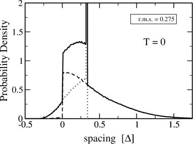
FIG. 1.: CB peak spacing distribution obtained using the CEI model (Eq. 1) with $T\!=\!0$ and $J_{S}\!=\!0.32\Delta$ ($r_{s}\!\approx\!1.5$). The dashed (dotted) line shows the $N$ even (odd) contribution (each spacing corresponds to a $N\!-\!1\!\rightarrow\!N\!\rightarrow\!N\!+\!1$ transition). Notice that the strong even/odd effect predicted by the CI model is significantly reduced and that the $\delta$-function in the odd distribution persists—but is shifted by $J_{S}$. The zero in the horizontal axis corresponds to $2E_{C}$ in the CI model.

The $T\!=\!0$ distribution shown in Fig. 1 will remain a good description so long as the contribution from the excited states can be ignored. To estimate that, let us calculate the average occupation ${\cal P}$ of the first excited state assuming that only it and the GS are relevant. In the CI model, the energy gap $\delta$ between those states is $\delta\!=\!\Delta\varepsilon$ where $\Delta\varepsilon$ is the single-particle energy spacing between the top levels. Using the GUE Wigner-Dyson distribution for $\Delta\varepsilon$—broken time-reversal symmetry is assumed throughout—we find ${\cal P}\!=\!0.02$ for $k_{B}T\!=\!0.1\Delta$. Thus, the excited states can indeed be ignored for $k_{B}T\!\leq\!0.1\Delta$. This is not the case in the CEI model, where $\delta$ gets reduced by the exchange interaction. For instance, for $N$ even, $\delta\!=\!|\Delta\varepsilon\!-\!2J_{S}|$ and ${\cal P}\!=\!0.14$ with $J_{S}\!=\!0.32\Delta$. Therefore, exchange not only modifies the $T\!=\!0$ distribution but makes the temperature effect stronger.

Furthermore, at finite temperature, the peak position involves the change in free energy of the QD upon adding a particle. Then, the spin degeneracy should play an important role through the entropy contribution. [19, 20, 21] Let us consider the regime $\Gamma\ll k_{B}T,\Delta\ll E_{C}$, where $\Gamma$ is the total with of a level in the QD. Near the CB peak corresponding to the $N\!-\!1\!\rightarrow\!N$ transition, the linear conductance is given by [20, 22]

$$G({\cal N})\!=\!\frac{e^{2}}{\hbar k_{B}T}\,P_{\mathrm{e}q}^{N}\,\sum_{\alpha}{\frac{\Gamma_{\alpha}^{L}\Gamma_{\alpha}^{R}}{\Gamma_{\alpha}^{L}\!+\!\Gamma_{\alpha}^{R}}\,w_{\alpha}}$$ (2)

with $\Gamma^{L(R)}_{\alpha}$ the partial width of the single-particle level $\alpha$ due to tunneling to the left (right) lead and

$$w_{\alpha}\!=\!\sum_{i,j,\sigma}{F_{\mathrm{e}q}(j|N)\left|\langle\Psi_{j}^{N}|c_{\alpha,\sigma}^{\dagger}|\Psi_{i}^{N\!-\!1}\rangle\right|^{2}[1\!-\!f(\epsilon_{j}\!-\!\epsilon_{i})]}.$$ (3)

Here $P_{\mathrm{e}q}^{N}$ is the equilibrium probability that the QD contains $N$ electrons, ${\hat{H}}_{\mathrm{Q}D}|\Psi_{j}^{N}\rangle\!=\!\epsilon_{j}|\Psi_{j}^{N}\rangle$, $F_{\mathrm{e}q}(j|N)$ is the conditional probability that the eigenstate $j$ is occupied given that the QD contains $N$ electrons, and $f(\epsilon)\!=\!\{1\!+\exp[(\epsilon-\!E_{F})/k_{B}T]\}^{-1}$. Since near the peak only the states with $N\!-\!1$ and $N$ electrons are relevant, we have $P_{\mathrm{e}q}^{N}\!\simeq\!f({\cal F}_{N}\!-\!{\cal F}_{N\!-\!1})$ with ${\cal F}_{N}$ the canonical free energy of the QD. [20] To make the dependence on ${\cal N}$ explicit, let us denote by $\{E_{j}\}$ the eigenenergies of ${\hat{H}}_{\mathrm{Q}D}$ without the charging energy term. Then, $\epsilon_{j}\!-\!\epsilon_{i}\!=\!E_{j}^{N}\!-\!E_{i}^{N\!-\!1}\!+\!2E_{C}\delta{\cal N}$ and ${\cal F}_{N}\!-\!{\cal F}_{N\!-\!1}\!=\!\mu_{N}\!+\!2E_{C}\delta{\cal N}$ with $\delta{\cal N}\!=\!(N\!-\!\frac{1}{2})\!-\!{\cal N}$ and $\mu_{N}\!=\!E_{j}^{N}\!-\!E_{i}^{N\!-\!1}\!+\!k_{B}T\ln\!\left[F_{\mathrm{e}q}(j|N)/F_{\mathrm{e}q}(i|N\!-\!1)\right]$ for any $i$ and $j$. The contribution of the transition $i\!\rightarrow\!j$ to the conductance reaches its maximum when

$$E_{F}\!=\!E_{j}^{N}\!-\!E_{i}^{N\!-\!1}\!+\!\frac{k_{B}T}{2}\ln\left[\frac{F_{\mathrm{e}q}(j|N)}{F_{\mathrm{e}q}(i|N\!-\!1)}\right]\!+\!2E_{C}\delta{\cal N}.$$ (4)

In the particular case where the transition between GS dominates, and taking the spin degeneracy into account, the CB peak position is given by

$$E_{F}\!=\!E_{\scriptscriptstyle GS}^{N}\!-\!E_{\scriptscriptstyle GS}^{N\!-\!1}\!-\!\frac{1}{2}k_{B}T\ln\left[\frac{2S_{\scriptscriptstyle GS}^{N}\!+\!1}{2S_{\scriptscriptstyle GS}^{N\!-\!1}\!+\!1}\right]\!+\!2E_{C}\delta{\cal N}.$$ (5)

We see that the peak is shifted with respect to its position at $T\!=\!0$ by an amount depending on the change of the spin of the QD.[19, 20, 21] Because the r.m.s. of the PSD is $\!\sim\!0.3\Delta$ (see Fig. 1), this shift is significant even for $k_{B}T\!\sim\!0.1\Delta$. In addition, while in the CI model this introduces only a constant shift between the even and odd distributions, in the CEI model it changes the shape of both distributions since different spin transitions contribute to each one.

Note that because of this shift, the on-peak conductance is renormalized.[19, 20] Since different spin transitions lead to different renormalizations, the average conductance peak depends not only on the average coupling to the leads but also on $J_{S}$ and on the statistics of the spectrum. This explains the small deviations observed[23] at low temperature from the values predicted in the absence of the exchange interaction (in particular the increase in Fig. 2 of Ref. [23]).

In the general case more than one transition contributes to the conductance, and the CB peak position must be determined by maximizing Eq.(2) with respect to ${\cal N}$. For simplicity, we restrict ourselves to the case where only the GS and first two excited states are relevant. By comparing the peak spacing distribution with and without including the second excited state, we found that this is the case for $k_{B}T\leq 0.2\Delta$, which is close to the experimental regime.

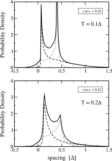
FIG. 2.: Finite temperature CB peak spacing distribution obtained using the CEI model [Eq. (1)]. Here $J_{S}\!=\!0.32\Delta$ and $k_{B}T\!=\!0.1\Delta$ $(0.2\Delta)$ in the top (bottom) plot. Notice that the $\delta$-function is smeared out and shifted by $k_{B}T\ln 2$ and that the even distribution develops a peak.

Figure 2 shows the PSD for non-zero temperature. The value $J_{S}\!=\!0.32\Delta$ corresponds to a gas parameter $r_{s}\!\sim\!1.5$. As expected, the sharp features are smeared out by temperature, including the $\delta$-function in the odd distribution. But more important, they are shifted due to the entropic term in (5). This is particularly clear for the peak associated with the $\delta$-function: it occurs at $J_{S}$ in Fig. 1 but at $J_{S}\!+\!k_{B}T\ln 2$ in Fig. 2 (the $\delta$-function is always associated with the spin transition $0\!\rightarrow\frac{1}{2}\!\rightarrow 0$). There are two other important effects worth comment: a) the even distribution develops a peak at small spacings while the odd one gets broader—in particular, at $k_{B}T\!=\!0.2\Delta$ the maximum of the total distribution is dominated by the even distribution, in contrast to what occurs at $T\!=\!0$; b) the relative weight of the long tail of the even distribution is strongly reduced and the distribution becomes more symmetric.

The peak in the even distribution arises from cases where $S\!=\!1$ and $S\!=\!0$ states are (almost) degenerate—it corresponds to the sharp jump at zero spacing in Fig. 1. According to Eq. (4) the CB peak is shifted by $\frac{1}{2}k_{B}T\ln(4/2)$ in that case, which gives a shift of $k_{B}T\ln 2$ for the peak in the PSD. The deviation from the $T\!=\!0$ result is still noticeable for $k_{B}T\sim 0.05\Delta$ (data not shown) which is the temperature in Ref.[6]. We found that the r.m.s. of the total distribution decreases monotonically when increasing $T$ in the range $k_{B}T\leq 0.2\Delta$, in contrast to the results obtained for the CI model.[25] The available experimental data[4] cannot discern this difference. An expected effect of the temperature is to increase the probability that $S\!=\!1$. This can be easily estimated by calculating the average probability $\langle F_{\mathrm{e}q}(S\!=\!1|N)\rangle$. We find $\langle F_{\mathrm{e}q}(S\!=\!1|N)\rangle\!=\!0.21(0.31)$ for $k_{B}T\!=\!0\ (0.1\Delta)$.

So far we have considered only the mean value of the residual interactions. It is clear that even at this level of approximation, the finite temperature PSD is quite different from the widely used $T\!=\!0$ CI model result: we should expect only a weak even/odd effect or asymmetry in the experimental data for $k_{B}T\!\hbox{\lower 3.44444pt\hbox{$\,\buildrel>\over{\sim}\,$}}\!0.2\Delta$.

Nevertheless, the distribution still does not agree with the one observed experimentally. Thus, we must go to the next level of approximation and include the leading order corrections to ${\hat{H}}_{\mathrm{Q}D}$. There are three contributions that lead to corrections of order $\Delta/\sqrt{g}$ to the spacing: 1) the “scrambling” of the spectrum when adding an electron to the QD that originates in the change of the charge distribution in the QD;[8] 2) the change in the single-electron energies when the gate voltage is swept;[15] 3) the fluctuation of the diagonal part of the $e$-$e$ interaction.[14] After including them, the Hamiltonian of the QD reads[18]

$${\hat{H}}_{\mathrm{Q}D} \!=\! {\hat{H}}_{\mathrm{Q}D}^{(0)}\!+\!\frac{1}{2}\sum_{\alpha,\beta,\gamma,\delta}{H_{\alpha,\beta,\gamma,\delta}^{(1/g)}\;\;c^{\dagger}_{\delta,\sigma}c^{\dagger}_{\gamma,\sigma^{\prime}}c_{\beta,\sigma^{\prime}}c_{\alpha,\sigma}}$$ (7)

$$\!+\!\sum_{\alpha,\beta,\sigma}\,{c^{\dagger}_{\alpha,\sigma}c_{\beta,\sigma}\,[(\hat{n}-{\cal N}){\cal X}^{0}_{\alpha,\beta}\!+\!\delta{\cal N}\,{\cal X}^{1}_{\alpha,\beta}}]$$

where, because of the fluctuations of the single-electron wavefunctions, the matrix elements $H_{\alpha,\beta,\gamma,\delta}^{(1/g)}$ and ${\cal X}^{j}_{\alpha,\beta}$ are gaussian random variables. They are characterized by ${\mathrm{v}ar}({\cal X}^{j}_{\alpha,\beta})\!=\!b_{jj}\Delta^{2}/g$ and ${\mathrm{v}ar}(H_{\alpha,\beta,\gamma,\delta}^{(1/g)})\!=\!c_{2}\Delta^{2}\ln({\tilde{c}_{2}}g)/g^{2}$; their mean values can be included in the definition of $E_{C}$ and $J_{S}$, so that $\langle H_{\alpha,\beta,\gamma,\delta}^{(1/g)}\rangle\!=\!\langle{\cal X}^{j}_{\alpha,\beta}\rangle\!=\!0$. Only the diagonal terms of the residual interaction (i.e. those where the operators $c^{\dagger}$ and $c$ are paired) are included in Eq. (7)—the off-diagonal terms can be neglected when calculating the PSD.[13, 16] Here, $\delta{\cal N}$ is taken with respect to the state with $N$ electrons. We use $g\!=\!0.384\sqrt{N/2}$ for the dimensionless conductance, which corresponds to a disc geometry.[18, 8] The coefficients $b_{jj}$, $c_{2}$ and ${\tilde{c}_{2}}$ are geometry-dependent. We estimate[16] $b_{00}\!\simeq\!0.01$,[24] $c_{2}\!\simeq\!0.003$, ${\tilde{c}_{2}}\!\simeq\!37$ for the experiment in Ref. [3], and we assume $b_{11}\!=\!b_{00}$. Notice that the magnitude of the “scrambling” and “gate” effects [last term in Eq. (7)] are much smaller than used previously in the literature.[15, 25]

Figure 3 shows the PSD including these corrections to the CEI model. The additional fluctuations increase the smearing of the remaining pronounced features of the distribution as well as of its r.m.s.. The distribution is less asymmetric but the even/odd effect is still noticeable—it should be kept in mind that the experimental noise will contribute significantly to this smearing. At $k_{B}T\!=\!0.2\Delta$ the peak of the distribution is still dominated by the even distribution. It is important to emphasize that this particular feature is exclusively related to the temperature effect. A detailed analysis of the experimental data of Ref. [3] shows[17] that the least noisy data present this signature and that the r.m.s. is of order of $0.25\Delta$, which is consistent with the prediction of this approach.[26] Furthermore, it is clear from the figures that the temperature effect is the main cause of the deviation from the CEI model result.

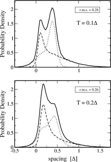
FIG. 3.: Finite temperature CB peak spacing distribution obtained from the Hamiltonian (Eq. 7) with $N\!=\!500$ ($g\!\approx\!6$), $J_{S}\!=\!0.32\Delta$ and $k_{B}T\!=\!0.1\Delta$ $(0.2\Delta)$ in the top (bottom) plot. Notice that both the even/odd effect and the asymmetry are small.

In conclusion, we have shown that the presence of the exchange interaction imposes a more restrictive condition on $T$ for observing GS properties in QDs. In particular, most of the experiments done so far require including temperature effects for their interpretation. The observed PSD seems to be the result of the addition of several small contributions.

We appreciate helpful discussions with D. Ullmo, L. I. Glazman and I. L. Aleiner. GU acknowledges partial support from CONICET (Argentina). This work was supported in part by the NSF (DMR-0103003).

REFERENCES

- [1] L. P. Kouwenhoven, C. M. Marcus, P. L. McEuen, S. Tarucha, R. M. Westervelt, and N. S. Wingreen, in Mesoscopic Electron Transport, edited by L. L. Sohn, L. P. Kouwenhoven, and G. Schön (Kluwer, New York, 1997), pp. 105–214.
- [2] U. Sivan, R. Berkovits, Y. Aloni, O. Prus, A. Auerbach, and G. Ben-Yoseph, Phys. Rev. Lett. 77, 1123 (1996).
- [3] S. R. Patel, S. M. Cronenwett, D. R. Stewart, A. G. Huibers, C. M. Marcus, C. I. Duruoz, J. S. Harris, K. Campman, and A. C. Gossard, Phys. Rev. Lett. 80, 4522 (1998).
- [4] S. R. Patel, D. R. Stewart, C. M. Marcus, M. Gokcedag, Y. Alhassid, A. D. Stone, C. I. Duruos, and J. J. S. Harris, Phys. Rev. Lett. 81, 5900 (1998).
- [5] F. Simmel, D. Abusch-Magder, D. A. Wharam, M. A. Kastner, and J. P. Kotthaus, Phys. Rev. B 59, R10441 (1999).
- [6] S. Lüscher, T. Heinzel, K. Ensslin, W. Wegscheider, and M. Bichler, Phys. Rev. Lett. 86, 2118 (2001).
- [7] O. Prus, A. Auerbach, Y. Aloni, U. Sivan, and R. Berkovits, Phys. Rev. B 54, R14289 (1996).
- [8] Y. M. Blanter, A. D. Mirlin, and B. A. Muzykantskii, Phys. Rev. Lett. 78, 2449 (1997); Phys. Rev. B 63, 235315 (2001).
- [9] R. Berkovits, Phys. Rev. Lett. 81, 2128 (1998).
- [10] P. W. Brouwer, Y. Oreg, and B. I. Halperin, Phys. Rev. B 60, R13977 (1999).
- [11] H. U. Baranger, D. Ullmo, and L. I. Glazman, Phys. Rev. B 61, R2425 (2000).
- [12] I. L. Kurland, I. L. Aleiner, and B. L. Altshuler, Phys. Rev. B 62, 14886 (2000).
- [13] P. Jacquod and A. D. Stone, Phys. Rev. Lett 84, 4951 (2000); also cond-mat/0102100 (unpublished)
- [14] D. Ullmo and H. U. Baranger, cond-mat/0103098 (unpublished).
- [15] R. O. Vallejos, C. H. Lewenkopf, and E. R. Mucciolo, Phys. Rev. Lett. 81, 677 (1998); Phys. Rev. B 60, 13682 (1999).
- [16] G. Usaj and H. U. Baranger (unpublished).
- [17] T. T. Ong, H. U. Baranger, D. M. Higdon, S. R. Patel, and C. M. Marcus (unpublished).
- [18] I. L. Aleiner, P. W. Brouwer, and L. I. Glazman, cond-mat/0103008 (unpublished) and references therein.
- [19] L. I. Glazman and K. A. Matveev, Pis’ma Zh. Éksp. Teor. Fiz. 48, 403 (1988), [JETP Lett. 48, 445 (1988)].
- [20] C. W. J. Beenakker, Phys. Rev. B 44, 1646 (1991).
- [21] H. Akera, Phys. Rev. B 59, 9802 (1999).
- [22] Y. M. Meir, N. S. Wingreen, and P. A. Lee, Phys. Rev. Lett. 66, 3048 (1991).
- [23] J. A. Folk, C. M. Marcus, and J. S. Harris, cond-mat/0008052 (unpublished).
- [24] This coefficient is difficult to evaluate since that requires calculating the electrostatic potential of a set of conductors (QD+gates) in a particular geometry. However, it is possible to estimate upper and lower bounds on its value. [16] For an isolated QD it can be evaluated explicitly, giving for an ellipsoidal geometry.
- [25] Y. Alhassid and S. Malhotra, Phys. Rev. B 60, R16316 (1999).
- [26] In the experiments cited, is greater than but the experimental noise should also be included.