[

Order from disorder: Quantum spin gap in magnon spectra of LaTiO₃

Abstract

A theory of the anisotropic superexchange and low energy spin excitations in a Mott insulator with $t_{2g}$ orbital degeneracy is presented. We observe that the spin-orbit coupling induces frustrating Ising-like anisotropy terms in the spin Hamiltonian, which invalidate noninteracting spin wave theory. The frustration of classical states is resolved by an order from disorder mechanism, which selects a particular direction of the staggered moment and generates a quantum spin gap. The theory explains well the observed magnon gaps in LaTiO₃. As a test case, a specific prediction is made on the splitting of magnon branches at certain momentum directions.

]

The recent renaissance in the study of transition metal oxides has emphasized the important role being played by the orbital degeneracy inherent to perovskite lattices (see for review  [1, 2]). First of all, the type of spin structure and the character of spin excitations crucially depend on the orientation of occupied orbitals [3, 4]. Second, the excitations in the orbital sector get coupled to the other degrees of freedom (electronic, lattice, spin) and might therefore strongly modify their excitation spectrum. Some examples are the anomalous magnon softening  [5] and incoherent charge transport  [6] due to low-energy orbital fluctuations in ferromagnetic manganites, and the formation of orbital polarons [7].

The calculation of the spin excitation spectrum in systems with orbital degeneracy is somewhat involved even at the half filled, insulating limit. That is due to the peculiar frustrations of superexchange interactions  [8], which lead to the infrared divergences when a linear spin wave theory is applied. In systems with $e_{g}$ orbital degeneracy the frustration is resolved by a specific, directional orbital ordering thus breaking the cubic symmetry of spin exchange bonds [9]. The transition metal oxides with $t_{2g}$ orbitals exhibit different and more challenging phenomena. This occurs due to the relative weakness of the Jahn-Teller coupling in this case, and due to the higher degeneracy and additional symmetry of $t_{2g}$ orbitals [10]. As a result, the orbitals may form the novel, coherent orbital-liquid state stabilized by quantum effects, as observed in spin the $S=1/2$ Mott insulator LaTiO₃ [11].

LaTiO₃ shows a spin order of G-type with magnon excitations characteristic for a simple cubic lattice. Despite three dimensionality of magnon spectra, the spin reduction is unusually large (much larger than in two dimensional cuprates), which has been explained in terms of fluctuating orbital state in this material [11, 10]. The present paper concerns with the origin of the small spin gap observed in LaTiO₃. This would not be an issue in a conventional case with static orbital order: The latter lowers a symmetry of the crystal and induces a spin anisotropy via the spin-orbit coupling, resulting naturally in a classical gap in the magnon spectra. Orbital order is however not observed in LaTiO₃, and the way how the staggered moment chooses one out of three equivalent cubic axes as the easy one is not that obvious. Indeed, it is shown below that the anisotropic Hamiltonian induced by spin-orbit coupling has a perfect cubic symmetry in the orbital liquid state, and a conventional spin wave theory gives in fact no magnon gap. We argue that the magnon gap and the selection of the easy magnetization axis in LaTiO₃ are nontrivial effects of quantum origin generated by the order from disorder mechanism.

We begin with the derivation of the effective spin Hamiltonian in $t_{2g}$ systems. Quite generally, it consists of the isotropic superexchange of Heisenberg form, and the anisotropic spin exchange Hamiltonian. The latter, which is of our present interest, results from higher order processes involving both the spin-orbit coupling

$$H_{so}=-\lambda\sum_{i}({\bf S}_{i}{\bf l}_{i})$$ (1)

and the isotropic superexchange. Here the operator ${\bf l}_{i}$ is the effective angular momentum ($l=1$) of $t_{2g}$ level, and ${\bf S}$ being a spin one-half of the Ti³⁺ ion. The isotropic superexchange in orbitally degenerate systems strongly depends on the orbital structure. In general it can be written as:

$$H_{\rm SE}^{ij}=\frac{4t^{2}}{U}[({\bf S}_{i}{\bf S}_{j}+\frac{1}{4})\hat{J}_{ij}^{(\gamma)}~{}+~{}\frac{1}{2}\hat{C}_{ij}^{(\gamma)}]~{},$$ (2)

where the orbital operators $\hat{J}_{ij}^{(\gamma)}$ and $\hat{C}_{ij}^{(\gamma)}$ depend on bond directions $\gamma(=a,b,c)$. In a $t_{2g}$ system like the titanates they are given by the following expressions:

$$\hat{J}_{ij}^{(\gamma)} = \frac{1}{2}(r_{1}+r_{2})(P_{ij}+K_{ij})^{(\gamma)}$$ (4)

$$-\frac{1}{3}(r_{2}-r_{3})P_{ij}^{(\gamma)}-\frac{1}{4}(r_{1}-r_{2})(n_{i}+n_{j})^{(\gamma)},$$

$$\hat{C}_{ij}^{(\gamma)} = \frac{1}{2}(r_{1}-r_{2})(P_{ij}+K_{ij})^{(\gamma)}$$ (6)

$$+\frac{1}{3}(r_{2}-r_{3})P_{ij}^{(\gamma)}-\frac{1}{4}(r_{1}+r_{2})(n_{i}+n_{j})^{(\gamma)},$$

The coefficients $r_{1}=1/(1-3\eta)$, $r_{2}=1/(1-\eta)$ and $r_{3}=1/(1+2\eta)$ originate from the Hund’s splitting of the excited $t_{2g}^{2}$ multiplet via $\eta=J_{H}/U$. The operators $P_{ij}^{(\gamma)}$, $K_{ij}^{(\gamma)}$ and $n_{i}^{(\gamma)}$ can conveniently be represented in terms of spinless fermions $a_{i}$, $b_{i}$, $c_{i}$ corresponding to $t_{2g}$ levels of $yz$, $xz$, $xy$ symmetry, respectively. (This notation is motivated by the fact that each $t_{2g}$ orbital is orthogonal to one of the cubic axes $a$,$b$,$c$). Namely,

$$P_{ij}^{(c)} = n_{ia}n_{ja}+n_{ib}n_{jb},$$ (7)

$$K_{ij}^{(c)} = a_{i}^{\dagger}b_{i}b_{j}^{\dagger}a_{j}+b_{i}^{\dagger}a_{i}a_{j}^{\dagger}b_{j},$$ (8)

$$n_{i}^{(c)} = n_{ia}+n_{ib}$$ (9)

for the pair along the $c$ axis. Similar expressions are obtained for the exchange bonds along the axes $a$ and $b$, by replacing orbital fermions $(a,b)$ in Eqs.(5) by $(b,c)$ and $(c,a)$ pairs, respectively. Since the parameter $\eta\equiv J_{H}/U\sim 0.16$ only [12], we will neglect the Hund’s coupling corrections. This results in a simple expressions as obtained in [10]:

$$\hat{J}_{ij}^{(c)} = n_{ia}n_{ja}+n_{ib}n_{jb}+a_{i}^{\dagger}b_{i}b_{j}^{\dagger}a_{j}+b_{i}^{\dagger}a_{i}a_{j}^{\dagger}b_{j},$$ (10)

$$\hat{C}_{ij}^{(c)} = -\frac{1}{2}(n_{ia}+n_{ib}+n_{ja}+n_{jb}).$$ (11)

The Eq.(7) is actually unessential for our purpose. Summed over bonds, this term gives the energy of the classical Néel state.

To complete the definitions, we express the angular momentum operator in Eq.(1) as follows:

$$l_{i}^{z}=i(a_{i}^{\dagger}b_{i}-b_{i}^{\dagger}a_{i}),l_{i}^{x}=i(b_{i}^{\dagger}c_{i}-c_{i}^{\dagger}b_{i}),l_{i}^{y}=i(a_{i}^{\dagger}c_{i}-c_{i}^{\dagger}a_{i}),$$ (12)

and notice finally that the fermions must satisfy a local constraint, $n_{ia}+n_{ib}+n_{ic}=1$.

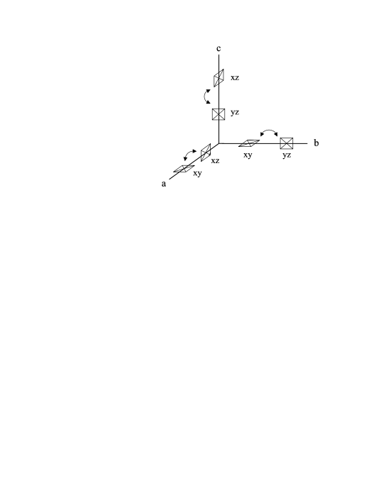
FIG. 1.: On every bond of cubic crystal, two out of three $t_{2g}$ orbitals are equally involved in the superexchange and may resonate. The same two orbitals select also a particular component of angular momentum.

To proceed further we need to specify the orbital state. The two most important features of the interactions in the present model can be observed from Eqs.(2,6): i)The classical Néel state (consider $\left\langle{\bf S}_{i}{\bf S}_{j}\right\rangle=-1/4$) is infinitely degenerate in the orbital sector, thus strong spin fluctuations must be present in the ground state to provide a dynamical splitting of orbital levels. ii)Special to $t_{2g}$ systems, every bond is represented by a particular pair of equivalent orbitals (see Fig.1 and Eq.(6)), which may form dynamical orbital singlet or triplet bonds. (In fact, the orbital operators $\hat{J}_{ij}^{(\gamma)}$ may be represented in a SU(2) symmetric form [10]). This additional symmetry brings up an intrinsic quantum dynamics into $t_{2g}$ orbital physics, contrasting it to a classical behaviour of $e_{g}$ systems. As described in [10], a composite spin-orbital excitation (an analogy to a SU(4) excitation [13]), which consists of a spin fluctuation accompanied by the formation of dynamical orbital bonds, best optimizes the superexchange energy. In that orbital liquid picture cubic symmetry remains unbroken. Angular momentum l is however fully quenched in the ground state, and it’s fluctuation spectrum extends up to characteristic energies of about $W_{orb}\sim 4t^{2}/U$. Last important remark concerns with spin-orbital separation: While the large energy ($\sim W_{orb}$) behaviour of the model Eq.(2) is governed by a coupled spin-orbital dynamics, the underlying weak magnetic order results in a separation of low energy spin excitations forming magnons on scale $J$. Here $J$ is a pure spin exchange coupling, $J({\bf S}_{i}{\bf S}_{j})$, which is obtained by averaging Eq.(6) over fast orbital dynamics. It has been found that indeed $J\ll W_{orb}$ [10], and this justifies the adiabatic approximation used below to derive an effective spin anisotropy Hamiltonian.

By symmetry, the anisotropic pairwise interactions for spins one-half in a cubic crystal must have the form

$$H_{ani}=A(\sum_{\langle ij\rangle_{a}}S_{i}^{x}S_{j}^{x}~{}+~{}\sum_{\langle ij\rangle_{b}}S_{i}^{y}S_{j}^{y}~{}+~{}\sum_{\langle ij\rangle_{c}}S_{i}^{z}S_{j}^{z}).$$ (13)

This interaction follows in the present model from spin-orbit corrections to the superexchange, shown in Fig.2. Only two of them, diagrams a) and c) do actually contribute to the anisotropy constant $A$. Consider the pair $\langle ij\rangle\parallel c$. The result is $H_{ani}^{ij}=AS_{i}^{z}S_{j}^{z}$ with $A=\lambda^{2}(2\Lambda_{z}^{(c)}-\Lambda_{x}^{(c)}-\Lambda_{y}^{(c)})/4$, where

$$\Lambda_{\alpha}^{(c)}=\langle l_{i}^{\alpha}\hat{J}_{ij}^{(c)}l_{i}^{\alpha}+l_{j}^{\alpha}\hat{J}_{ij}^{(c)}l_{j}^{\alpha}+l_{i}^{\alpha}l_{j}^{\alpha}\hat{J}_{ij}^{(c)}+\hat{J}_{ij}^{(c)}l_{i}^{\alpha}l_{j}^{\alpha}\rangle_{orb}~{}.$$ (14)

Here $\langle\cdot\cdot\cdot\rangle_{orb}$ implies the average over orbital fluctuations. The basic assumption in the above derivation is that these fluctuations are fast enough to enable us to integrate them out as far as we are concerned with the low energy, magnon like dynamics of the spin operators. Next, it is important to observe that both $l_{z}$ (see Eq.(8)) and $\hat{J}_{ij}^{(c)}$ operate on the same orbital doublet ($a,b$). One therefore obtains $\Lambda_{z}^{(c)}>\Lambda_{x}^{(c)}=\Lambda_{y}^{(c)}$. For the pairs $\langle ij\rangle\parallel a$ and $\langle ij\rangle\parallel b$, on the other hand, ($b,c$) and ($c,a$) doublets are more active, resulting in $AS_{i}^{x}S_{j}^{x}$ and $AS_{i}^{y}S_{j}^{y}$ interactions, respectively. The physical picture is that the anisotropic spin interaction arises here as an indirect coupling via fluctuations of the angular momentum of $t_{2g}$ level. In every direction one particular component among $l^{\alpha}$ in Eq.(8) is special, having more dispersive fluctuations in that direction, therefore the structure of Eq.(9) follows.

Eq.(10) can be expressed in terms of an on-site orbiton Green’s functions which we evaluate using constant density of states within the orbiton bands of width $W_{orb}$, as obtained in the large $N$ approximation [10]. This gives

$$A=f(4t^{2}/U)(\lambda/W_{orb})^{2}~{},$$ (15)

with the numerical factor $f\simeq 3$. We may notice, that $W_{orb}$ in this expression actually plays the role of a static splitting of levels in a conventional, orbitally ordered case. The estimation in Ref. [10] yields for the Heisenberg exchange constant $J\simeq 0.16(4t^{2}/U)$ and the orbiton bandwidth $W_{orb}\simeq 1.6(4t^{2}/U)$, thus the energy scale $4t^{2}/U\simeq 100$ meV follows using $J_{exp}=15.5\pm 1$ meV in LaTiO₃ [11]. With $\lambda=19$ meV [14], we then estimate $A\simeq 4.2$ meV for cubic anisotropy constant in LaTiO₃.

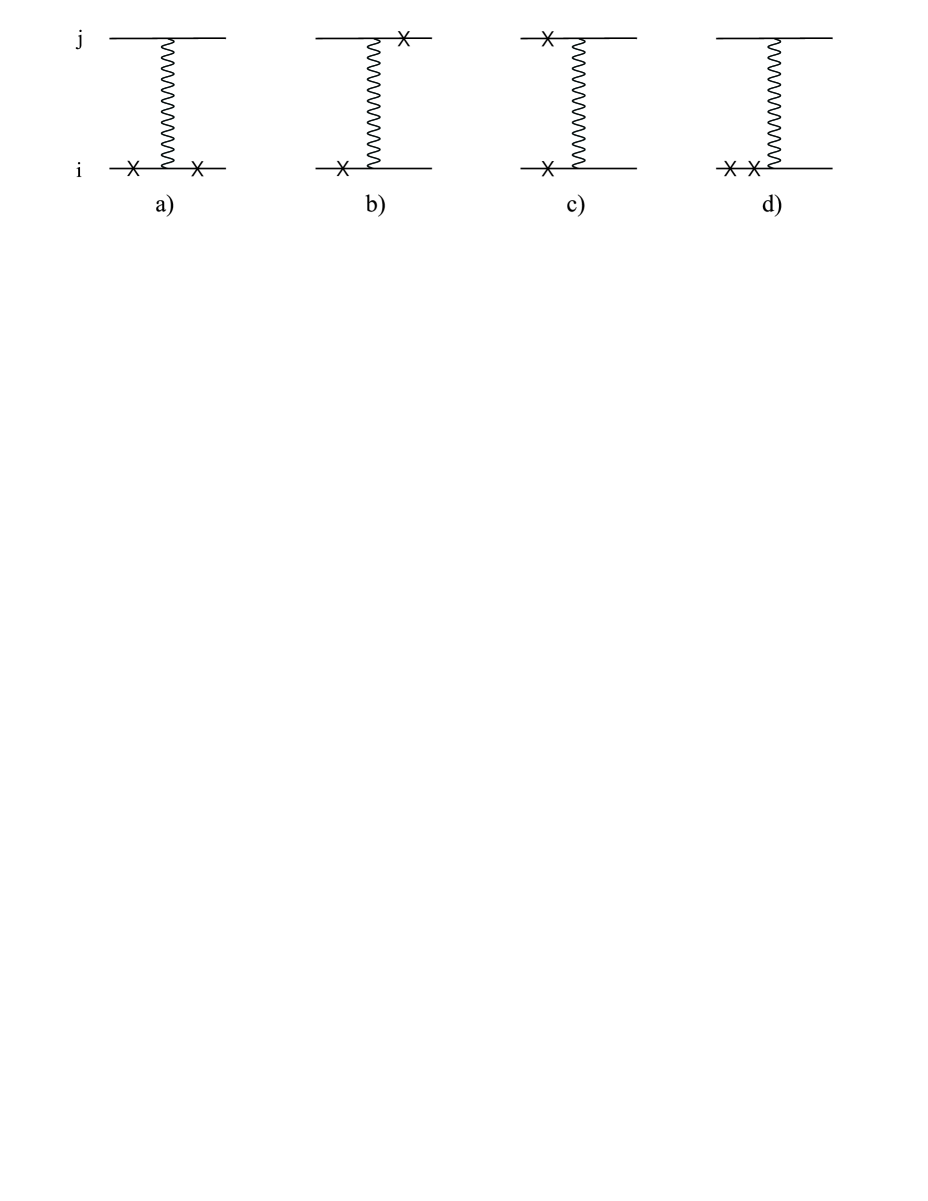
FIG. 2.: Lowest order spin-orbit corrections to the spin exchange Hamiltonian for a pair $\langle ij\rangle$. Wavy lines represent the isotropic superexchange in Eq.(2), solid lines are the orbiton on-site Green’s functions. The spin-orbit coupling in Eq.(1) is denoted by crosses.

We point out here a crucial difference between the present case and a canonical theory of the anisotropic superexchange interactions in orbitally nondegenerate systems like cuprates. In $e_{g}$ systems, one has to treat both symmetric and antisymmetric (Dzyaloshinskii-Moriya (DM) [15]) parts of the anisotropic superexchange on equal footing because of the intimate relationship between them [16], since both are due to the finite deviations (tilting of octahedra etc.) from the ideal structure. In the present $t_{2g}$ case these interactions are, however, decoupled: while the DM interaction vanishes by cubic symmetry, a symmetric superexchange anisotropy is fully operating. The key point here is that the $t_{2g}$ state manifold has an intrinsic angular momentum.

Now we consider how the interaction Eq.(9) will affect magnon excitations. Since spin symmetry is lowered to the discrete (cubic) one, a magnon gap is expected. A linear spin wave theory fails however to obtain it, because Eq.(9) acquires a rotational symmetry in the limit of classical spins. This results in an infinite degeneracy of classical states, and an accidental pseudo Goldstone mode appears, which is however not a symmetry property of the original quantum model Eq.(9). Villain’s order from disorder mechanism [17] comes into play at this point, selecting a particular classical state such that the fluctuations about this state give the largest energy gain, and opening also a magnon gap. To explore this point explicitly, we calculate quantum corrections to the ground state energy as a function of the angle $\theta$ between $c$ axis and the staggered moment. Assuming the latter is perpendicular to $b$ axis, we rotate globally a spin quantization axes as $S^{z}\rightarrow S^{z}\cos\theta-S^{x}\sin\theta$, $S^{x}\rightarrow S^{x}\cos\theta+S^{z}\sin\theta$, and observe that the magnon excitation spectrum has an explicit $\theta$-dependence:

$$\omega_{\bf p}(\theta)=zJS\{Y_{\bf p}(X_{\bf p}+2a\eta_{zx}\sin^{2}\theta)\}^{1/2}~{},$$ (16)

$$Y_{\bf p}=1-\gamma_{\bf p}+a(1-c_{y})~{},$$ (17)

$$X_{\bf p}=1+\gamma_{\bf p}+a(1+c_{x})~{}.$$ (18)

Here the ratio $a=A/3J$ quantifies the deviation from the Heisenberg limit, and $\eta_{zx}=(c_{z}-c_{x})/2$ , $\gamma_{\bf p}=(c_{x}+c_{y}+c_{z})/3$ , where $c_{\alpha}=\cos p_{\alpha}$ , and $z=6$. Calculating the zero point magnon energy, one obtains an effective potential for the staggered moment, which at small $\theta$ reads as a harmonic one: $E(\theta)=const+K_{eff}S^{2}\theta^{2}$, with an effective “spring” constant $K_{eff}=\frac{1}{2}zJa\kappa\equiv A\kappa$. The parameter $\kappa$ is given by

$$\kappa=\frac{1}{S}\sum_{\bf p}\eta_{zx}(Y_{\bf p}/X_{\bf p})^{1/2}~{}.$$ (19)

At small $a\ll 1$, in which case we are interested in, $\kappa\simeq 3aR/8S$, and $K_{eff}\simeq(R/8S)(A^{2}/J)$, with the numerical factor

$$R=\sum_{\bf p}(1+\gamma_{\bf p}^{2})(c_{z}^{2}-\gamma_{\bf p}^{2})/(1-\gamma_{\bf p}^{2})^{3/2}~{}\approx 0.44~{}.$$ (20)

The physical meaning of the above calculation is that zero point quantum fluctuations, generated by the interaction in Eq.(9), are enhanced when the staggered moment stays about a symmetric position (one of three cubic axes), and this leads to the formation of the energy profile of cubic symmetry. A breaking of this discrete symmetry results then in the magnon gap, which should be about $\sqrt{K_{eff}/M}$ with $1/M\sim zJ$ in the harmonic approximation. More quantitatively, the potential $E(\theta)$ can be associated with an effective uniaxial anisotropy term, $K_{eff}\sum_{\langle ij\rangle_{c}}S_{i}^{z}S_{j}^{z}$, generated in the symmetry broken phase. Therefore, one finds the magnon gap $\Delta=zJS\sqrt{2K_{eff}/3J}$, which is a linear function of the anisotropic interaction $A$:

$$\Delta=zJS\sqrt{2a\kappa}=A\sqrt{3RS}~{}.$$ (21)

Now we derive this result using a different approach. Namely, we write the equations of motion, $\omega S_{i}^{\alpha}=[S_{i}^{\alpha},H]$ with $H$ being the Heisenberg exchange plus $H_{ani}$ in Eq.(9), and account for the interaction between magnons and local fluctuations of the staggered moment $\delta S_{j}^{z}$, generated by $H_{ani}$, within the following approximation:

$$S_{i}^{x}\delta S_{j}^{z}\Rightarrow(\chi^{(\gamma)}+\Delta^{(\gamma)})S_{j}^{x}~{},$$ (22)

$$S_{i}^{y}\delta S_{j}^{z}\Rightarrow(\chi^{(\gamma)}-\Delta^{(\gamma)})S_{j}^{y}~{}.$$ (23)

Here $\gamma=a,b,c$ specifies the bond direction $\langle ij\rangle$, and the bond variables are defined as $\chi^{(\gamma)}=-\langle b_{i}^{\dagger}b_{j}\rangle$ , $\Delta^{(\gamma)}=-\langle b_{i}^{\dagger}b_{j}^{\dagger}\rangle$ , where $b_{i}$ is the Holstein-Primakoff boson operator. This linearization procedure leads to the magnon excitation spectrum

$$\omega_{\bf p}=zJS\{(Y_{\bf p}+a\kappa)(X_{\bf p}+a\kappa)\}^{1/2}~{},\\$$ (24)

where $\kappa=\kappa^{(a)}-\kappa^{(c)}$, and $\kappa^{(\gamma)}=(\chi^{(\gamma)}+\Delta^{(\gamma)})/S$. The key observation here is that the bond variables along the $c$ axis differ from those in directions perpendicular to the staggered moment. Indeed, calculating bond variables $\chi^{(\gamma)}$ and $\Delta^{(\gamma)}$ by using the spectrum in Eq.(19), one finds $\kappa$ to be positive, given by the selfconsistent equation:

$$\kappa=\frac{1}{S}\sum_{\bf p}\eta_{zx}(Y_{\bf p}+a\kappa)^{1/2}/(X_{\bf p}+a\kappa)^{1/2}~{}.$$ (25)

This is expected since the fluctuations originate mostly from $a$ and $b$ bonds in Eq.(9), once we have chosen the $c$ axis as an easy one. Thus $\kappa^{(a)}>\kappa^{(c)}$ follows.

Consider again the weak anisotropy case, $a\ll 1$. From equations (19) and (13,14) we read off the magnon gap $\Delta=zJS\sqrt{2a\kappa}$. Noticing also that Eq.(20) reproduces in this limit precisely the same parameter ${\kappa}$ defined in Eq.(15), we confirm finally our previous result, given by Eq.(17), for the magnon gap. Superior to the previous case, the latter solution gives not only the gap value, but also the full magnon spectrum Eq.(19), which we will discuss soon.

One may wonder about the behaviour of Eqs.(20,19) in another extreme limit, $a\gg 1$, where one is left with only the cubic term. Actually, the model defined in Eq.(9) is of certain interest by it’s own [18]. For $a\rightarrow\infty$, one finds that the solution of Eq.(20) saturates at the value $\kappa_{\infty}\simeq(2/\pi^{2}S)r_{S}$, where $r_{S}=\ln(4\pi\sqrt{S})-1$. The excitation spectrum in this limit is two-dimensional, $\omega_{\bf p}=2AS\{(1+\kappa_{\infty}-c_{y})(1+\kappa_{\infty}+c_{x})\}^{1/2}$, and it shows again the gap $\Delta=(4/\pi)A\sqrt{r_{S}S}$ of order $A$. The spin reduction due to the frustrations is found to be nonsingular for finite spin values. Although it is logarithmically diverging in the limit of large classical spins, $\delta S^{z}\rightarrow\frac{2}{\pi^{2}}\ln(4\pi\sqrt{S})$, the ratio $\delta S^{z}/S$ vanishes in this limit. Therefore, we believe that long range order in the “cubic” model with nearest-neighbor interactions is well defined for both one-half and large spins. It should be noticed, however, that the approximation used here is less accurate in the “cubic” limit, and we anticipate substantial incoherent features in the excitation spectrum, which is expected to show a pseudogap of about $\Delta$ and a full bandwidth $\omega_{max}\sim 4AS$.

Now we turn to the realistic case, LaTiO₃, and discuss the numbers. With $A\simeq 4.2$ meV estimated above, Eq.(17) gives $\Delta\simeq 3.4$ meV, which is in surprisingly good agreement with $\Delta_{exp}=3.3\pm 0.3$ meV [11]. We believe therefore that the quantum gap induced by the cubic anisotropy is the dominant contribution to the magnon gap in LaTiO₃ [19]. This can actually be tested experimentally. The point is that the spectrum $\omega_{\bf p}$ in Eq.(19) contains full information of the interaction in Eq.(9) on large energy scales, and it’s peculiar structure may manifest itself in a neutron scattering experiment. Namely, two magnon branches of a commensurate antiferromagnet are related to Eq.(19) as $\Omega_{1}({\bf p})=\omega_{\bf p}$ and $\Omega_{2}({\bf p})=\omega_{{\bf p}+{\bf Q}}$, where ${\bf Q}$ being the Néel vector. Because of the presence of $S^{x}$ and $S^{y}$ components in Eq.(9), the two branches are in fact degenerate only in the planes with $p_{x}=\pm p_{y}$, otherwise a splitting of these two modes is expected at large momenta. The splitting is largest along $[0,\pi,p_{z}]$ and equivalent lines and reaches a maximal value $2A\sim 8$ meV at the $p_{z}=\pi/2$ point. This may enable one to measure directly the value of the cubic anisotropy constant $A$, and quantify further the orbital liquid state in a such puzzling material like LaTiO₃.

We would like to emphasize that a small value of the spin gap in LaTiO₃ is very difficult to explain from the traditional point of view (see also the discussion in [11]). Indeed, large static orbital splitting of order of 150-200 meV would be required in order to suppress spin-space anisotropy and hence to explain the small magnon gaps as observed. However, such large splittings are very difficult to reconcile with the fact that neither orbital order nor any traces of related structural transitions have been detected. The orbital liquid concept naturally resolves this apparent conflict: The large orbital energy scale is generated in this picture by electronic correlations, and angular momentum is quenched dynamically, without static symmetry breaking.

To conclude, a theory of the anisotropic superexchange of $t_{2g}$ electrons in titanites is presented. This interaction introduces nontrivial frustration in low energy spin states. We have identified a mechanism which selects the easy magnetic axis in cubic crystal with disordered orbital states. The spin gap in LaTiO₃ is most likely of quantum origin, being thus as unique as the orbital state in this “simple” Mott insulator is. An experimental test of the theory is suggested.

We would like to thank B. Keimer for stimulating discussions. Discussions with C. Ulrich, R. Zeyher and J. van den Brink are also acknowledged.

REFERENCES

- [1] Y. Tokura and N. Nagaosa, Science 288,462 (2000).
- [2] K. I. Kugel and D. I. Khomskii, Sov. Phys. Usp. 25, 231 (1982).
- [3] J. B. Goodenough, Phys. Rev. 100, 564 (1955).
- [4] J. Kanamori, J. Phys. Chem. Solids 10, 87 (1959).
- [5] G. Khaliullin and R. Kilian, Phys. Rev. B 61, 3494 (2000).
- [6] S. Ishihara, M. Yamanaka, and N. Nagaosa, Phys. Rev. B 56, 686 (1997); R. Kilian and G. Khaliullin, Phys. Rev. B 58, R11841 (1998).
- [7] R. Kilian and G. Khaliullin, Phys. Rev. B 60, 13458 (1999); T. Mizokawa, D. I. Khomskii, G. A. Sawatzky, Phys. Rev. B 63, 024403 (2001).
- [8] L. F. Feiner, A. M. Oleś, and J. Zaanen, Phys. Rev. Lett. 78, 2799 (1997).
- [9] G. Khaliullin and V. Oudovenko, Phys. Rev. B 56, R14 243 (1997).
- [10] G. Khaliullin and S. Maekawa, Phys. Rev. Lett. 85, 3950 (2000).
- [11] B. Keimer et al., Phys. Rev. Lett. 85, 3946 (2000).
- [12] T. Mizokawa and A. Fujimori, Phys. Rev. B 54, 5368 (1996).
- [13] Y. Q. Li, M. Ma, D. N. Shi, and F. C. Zhang, Phys. Rev. Lett. 81, 3527 (1998); B. Frischmuth, F. Mila, and M. Troyer, Phys. Rev. Lett. 82, 835 (1999).
- [14] A. Abragam and B. Bleaney, Electron Paramagnetic Resonance of Transition Ions (Oxford University Press, New York, 1970).
- [15] T. Moriya, Phys. Rev. 120, 91 (1960).
- [16] I. Shekhtman, O. Entin-Wohlman, and Amnon Aharony, Phys. Rev. Lett. 69, 836 (1992).
- [17] For a discussion of the order from disorder phenomena in frustrated spin systems, see A. M. Tsvelik, Quantum Field Theory in Condensed Matter Physics (Cambridge University Press, Cambridge, 1995), Chap. 17, and references therein.
- [18] Problems with this model have been noticed long ago: See discussion of the “cubic” model in Ref. [2], p. 253.
- [19] Yet a complete description of the spin anisotropy in LaTiO3 should include also the Dzyaloshinskii-Moriya interaction in order to explain the weak ferromagnetism of this material. DM interaction becomes finite due to the small tilting of octahedra.