Universal fluctuations and extreme value statistics

Abstract

We study the effect of long range algebraic correlations on extreme value statistics and demonstrate that correlations can produce a limit distribution which is indistinguishable from the ubiquitous Bramwell-Holdsworth-Pinton distribution. We also consider the square-width fluctuations of the avalanche signal. We find, as recently predicted by T. Antal, M. Droz G. Györgyi and Z. Rácz for logarithmic correlated $1/f$ signals, that these fluctuations follow the Fisher-Tippett-Gumbel distribution from uncorrelated extreme value statistics.
PACS numbers: 05.65.+b,05.40.-a,05.50.+q,68.35.Rh

]

I Introduction

Three years ago Bramwell, Holdsworth and Pinton (BHP) published the remarkable discovery that the same functional form that describes the fluctuation spectrum of the energy injected in an experiment on turbulence also describes the fluctuations in the magnetization of the finite size two dimensional XY equilibrium model in the critical region below the Kosterlitz-Thouless transition temperature [1]. Since three dimensional turbulence and two dimensional magnetic equilibrium system appear to have very little in common, BHP made the reasonable suggestion that the origin of the identical functional form for the fluctuation spectra should be sought in the one thing the two systems appear to share, namely, scale invariance. This suggestion was supported by the subsequent finding that a long list of scale invariant (or nearly scale invariant) non-equilibrium as well as equilibrium systems exhibit the same BHP form for the fluctuation spectrum for certain quantities [2].

Nevertheless, not all critical systems fluctuates according to the BHP spectrum. This was made very explicit by Aji and Goldenfeld [3], who proffered the interesting suggestion that the reason the two dimensional (2d) XY-model and the driven turbulence experiment exhibit the same fluctuation spectrum could be that the 2d XY-model is the effective model for the turbulence experiment. Even if this is correct we still lack an explanation of why so many disparate systems [2] do exhibit BHP fluctuations.

The BHP functional form is similar to one of the asymptotic forms for extreme value statistics: the asymptote first discussed by Fisher and Tippett [5] and often referred to as the Gumbel distribution [6]. The BHP distribution is, however, not identical to the Fisher-Tippett-Gumbel (FTG) asymptote. Consider $T$ independent and identically distributed stochastic variables. Under certain conditions (essentially exponential tail) the $k$-th largest of the $T$ variables will be distributed according to the FTG asymptote with $k$ entering as a parameter. The BHP form can be thought of as corresponding to the somewhat uninterpretable case of $k=\pi/2$ [2].

As already alluded to in Ref. [2] the deviation between the BHP and the FTG form may be related to correlations. Our main aim in the present paper is to study this point in detail. We do that by simulating the so called Sneppen depinning model [7]. The power spectrum of the Sneppen model behaves like $1/f^{\beta}$ with $\beta\simeq 0.5$ for low frequencies corresponding to a very slow algebraic decay of the autocorrelation function (see e.g. [8]). We use the Sneppen model in the next section to demonstrate that extreme value statistics of $T$ strongly correlated exponentially distributed variables may follow the BHP form. Remarkably, Antal et al. [4] demonstrated analytically that, at least for a certain class of $1/f$ signals (periodic signals), the width-square fluctuations ($w_{2}$) of the signal follow the FTG distribution from extreme value statistics, though it is not clear why this should be the case. Inspired by this finding we study in Section III the width fluctuations of the avalanche signal in the Sneppen model. We find, contrary to the 1/f case studied by Antal et al., that the probability density function for $w_{2}$ in the Sneppen model is very well represented by the FTG distribution even for non-periodic signals. Section IV contains a discussion and our conclusions.

II Extreme value statistics and the Sneppen model

To investigate the relationship between extreme value statistics of correlated variables and the BHP probability density we consider now the simple 1+1 dimensional depinning model introduced by Sneppen [7]. The model is imagined to represent a one dimensional elastic interface moving transverse while acted upon by a set of random pinning forces, See Fig. 1a.

The model, which is discrete and very schematic, consists of $L$ sites in the $x$-direction and infinitely many sites in the $y$-direction. Each square on this semi-infinite lattice is assigned a random number, the pinning force, uniformly distributed on the interval $[0,1[$. The interface is represented by the set $\{(x,y)|y=h(x,t)\}$, where $h(x,t)$ denotes the “hight” of the interface above the $x$-axis at time $t$ at site $x$ along the $x$-axis. The initial configuration is $h(x,0)=0$ for $\forall\;x$. In each time step the interface site, $x_{s}$ with the smallest pinning force is located and the interface at this location is moved one step ahead, i.e., $h(x_{s},t)\mapsto h(x_{s},t)+1$. This may cause the neighbouring slope $|h(x_{s},t)-h(x_{s}-1,t)|$ (or $|h(x_{s}+1,t)-h(x_{s},t)|$) to exceed 1, in which case the interface at site $x_{s}-1$ is moved one step ahead, i.e. $h(x_{s}-1,t)\mapsto h(x_{s}-1,t)+1$ (and similar for the site $x_{s}+1$ if needed). The update of the nearest neighbour sites of $x_{s}$ may cause the slope on the next nearest sites to exceed 1. In which case the interface is moved ahead on these sites. This procedure is repeated until all slopes satisfy $h(x,t)-h(x-1,t)|\leq 1$ once again. The sequence of operations needed to make all slopes smaller than or equal to 1 after the update of site $x_{s}$ is denoted one time step. The number of sites updated during one time step is called a micro-avalanche. The number of sites being updated during the time step $t$ is called the size of the avalanche $s(t)$ and per definition the duration of each of these avalanches is the same, namely one time step.

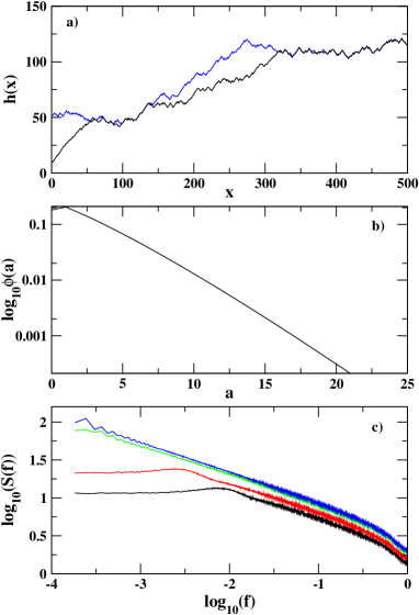
FIG. 1.: a) Snapshot of the sneppen interface $h(x)$ at two times 10000 timesteps apart, system size $L=500$. b) The PDF of the micro-avalanches in the sneppen model, system size $L=500$. c) The power spectrum of micro-avalanches for 4 different system sizes. From bottom to top $L=50,100,500,1000$.

The probability density function (PDF) for the size of the micro-avalanches is close to an exponential as seen in Fig. 1b and first reported in [7]. The individual micro-avalanches are strongly correlated in time. This is clearly seen from the power spectrum $S(f)$ of the temporal signal $s(t)$, see Fig. 1c. The low frequency behaviour of the power spectrum is approximately $S(f)\sim 1/\sqrt{f}$, indicative of slow algebraic decay of the auto-correlation function of the signal $s(t)\sim 1/\sqrt{t}$ (see e.g. [8]).

Let us now imagine that the activity of the model is monitored by some devise which has only a limited resolution. This might be modeled by assuming that the measured signal $\bar{S}_{T}(\tau)$, rather than consisting of the microscopic instantaneous activity $s(t)$, is given by the sum of activities within a time window of a certain size $T$:

$$\bar{S}_{T}(\tau)=\sum_{t=\tau}^{\tau+T}s(t).$$ (1)

This signal was among the set of quantities in Ref. [2] found to follow the BHP distribution for a certain range of window sizes $T$. That is, if $T$ is too small the PDF for $\bar{S}_{T}(\tau)$ is close to an exponential distribution. The central limit theorem will, however, cause the PDF for $\bar{S}_{T}(\tau)$ to approach a Gaussian when $T$ becomes large enough that correlations amongst the $s(t)$ entering the sum in Eq. 1 can be neglected. This deviation can be observed in Fig. 2a. Presumably the PDF for $S(T)$ would remain close to the BHP form even for $T\rightarrow\infty$ if the correlation time of the signal was infinite as it would be expected to be in the limit of infinite system size, see Fig. 1c.

Since, as seen in Fig. 2b, the functional form of the BHP distribution is close to the first FTG asymptote for extreme value statistics we proceed to investigate the extreme statistics of the correlated variables $s(t)$ generated by the Sneppen model. For the time windows considered for $\bar{S}_{T}(\tau)$ we define

$$M_{T}(\tau)=\max\{s(\tau),s(\tau+1),...,s(\tau+T)\}.$$ (2)

In Fig. 2b we show the scaled PDF for $M_{T}(\tau)$. First we compare the distribution of the sum and the max in Fig. 2a. We see that the distribution for $M_{T}(\tau)$ remain very close to the BHP distribution for all considered sampling sizes $T$, while the distribution for $\bar{S}_{T}(\tau)$ gradually deviates from the BHP as $T$ is increased. In Fig. 2b we demonstrate two interesting points. First that for system size $L=1000$ we are unable to make $T$ so large that the distribution for $M_{T}(\tau)$ deviates form the BHP form. No difference between the results for $T=5000$ and $T=10000$ can be detected. The size dependence is, however, detectable, as illustrated in the insert to Fig. 2b. We show here the PDF for smaller system sizes $L=500$ and $L=50$. The spatial extend of the system $L=50$ is now sufficiently small to destroy the long range temporal correlations as is seen from the fact that the PDF for $L=50$, $T=500$ follows the FTG form for uncorrelated extreme value statistics. We elaborate on the role of the correlations in the main frame of Fig. 2b. This figure demonstrates that the deviation between the PDF for $M_{T}(\tau)$ and the FTG form is indeed caused by the correlations of the Sneppen model. This conclusion is reached in the following way. We generate $T$ uncorrelated stochastic variables $\chi_{i}$ all drawn from the PDF for the individual micro-avalanches $s(t)$ (see Fig. 1b). The difference between

$$M_{uc}=\max\{\chi_{1},\chi_{2},...,\chi_{T}\}$$ (3)

and $M_{T}(\tau)$ is solely the correlations amongst the primary variables from which $M_{T}(\tau)$ is generated. Hence, given the exponential form of the PDF for the distribution of the individual micro-avalanches (see Fig. 1b) we expect the PDF for the uncorrelated extreme $M_{uc}$ to follow the FTG asymptote for large values of $T$. This is exactly what is found in Fig. 2b.

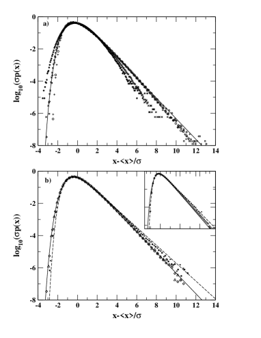
FIG. 2.: a) The PDF of $\bar{S}_{T}(\tau)$ for $T=50(+)$, $T=500(x)$ and $T=500(*)$ and the PDF of $\bar{M}_{T}(\tau)$ for $T=50\;(\circ)$, $T=500\;(\Box)$ and $T=5000\;(\diamond)$, the solid line is the BHP PDF. b) The PDF of $M_{T}(\tau)$ for $T=5000\;(\diamond)$ and $T=10000\;(\triangle)$ and the PDF of the decorrelated maximum $M_{u}c$ for $t=5000\;(*)$ and $T=10000\;(+)$, the solid line is the BHP form and the dashed line is the FTG form. The inset: The PDF of $M_{T}(\tau)$ for system sizes, $L=50$, $T=50\;(\circ)$ and $T=500\;(\bullet)$.

III The square width and extreme value statistics

In the present section we analyse the statistics of the fluctuations in the width of the avalanche signal $s(t)$ generated by the Sneppen model and of the $1/f$ signal $F(\tau)$ in Eq. 6 below. Our inspiration is from the beautiful paper by Antal, Droz, Györgysi and Rácz (ADGR) [4]. These authors demonstrated analytically that at least for a certain class of $1/f$ signals $h(t)$, the width-square

$$w_{2}(h)=\overline{[h(t)-\bar{h}]^{2}}$$ (4)

is distributed according to the FTG distribution. In Eq. 4 the over-bar denotes the following time average

$$\bar{h}={1\over T}\sum_{t=1}^{T}h(t).$$ (5)

The result by ADGR is striking since it is unclear how or if extreme value statistics is involved in some effective way in determening the distribution of $w_{2}$.

As a contribution to the investigation of the generality of the discovery by ADGR we studied $w_{2}$ for the signal $s(t)$. This signal is not $1/f$ but rather $1/\sqrt{f}$, and differs in this way from the class studied in Ref. [4]. As see in Fig. 3a $w_{2}$ for $s(t)$ does follow the FTG functional form except for very small sample sizes. This indicates that the ADGR result is more general than their calculation allows one to conclude. ADGR predicted analytically that this should be the case for periodic $1/f$ signals and they report that deviations are observed in simulations of non-periodic $1/f$ signals.

To address the question about deviations from the FTG form we show in Fig. 3b the fluctuations in $w_{2}$ for a $1/f$ signal of the type considered by Antal et al. We generated the signal as the “half integral” of white noise [9], i.e., the signal is obtained as a convolution between white noise and a propagator $G(t)$ which decays as an inverse square root:

$$F(\tau)=\lim_{T_{*}\rightarrow\infty}\sum_{t=\tau-T_{*}}^{\tau}G(\tau-t)\chi(t),$$ (6)

where $G(x)=1/\sqrt{x}$. We assume $\chi(t)$ to be uncorrelated and uniformly distributed on the interval $[-1,1]$ and in our simulations we truncate the sum in Eq. (6) at $T_{*}=2^{20}$.

One can calculate the PDF of the Fourier coefficients of the signal of length $T$ in Eq. (6) by performing a discrete Fourier analysis (note this amounts to assuming a signal of periodicity $T$)

$$\hat{F}(\omega)=\sum_{\tau=0}^{T}F(\tau)e^{-i\omega\tau}.$$ (7)

Averaging over the white noise $\chi(t)$ gives the following PDF for the Fourier amplitudes

$$p(|\hat{F}(\omega)|^{2}=R^{2})={3\omega\over\pi T}\exp\left(-{3\over\pi T}\omega R^{2}\right).$$ (8)

which demonstrates explicitly that the signal in Eq. (6) is of the type considered by ADGR [4].

We notice that the simulated distribution for $w_{2}$ in Fig. 3b for all sample sizes $T$ deviates from the FTG form predicted by Antal et al. This was indeed noticed by ADGR (their Fig. 1) and ascribed to the difference between the assumed periodic boundary condition needed to perform analytical calculation of the PDF of $w_{2}$ and the non-periodic signal simulated. This problem appears not to arise in case of the Sneppen model, where Fig. 3a shows that the PDF for $w_{2}$ follows the FTG form as soon as $T$ is of order 500 or larger. We recall that the difference between the signal in the Sneppen model and the signal in Eq. (6) is that the Sneppen signal is algebraically correlated with an autocorrelation function that decays like one over the square root of time whereas the $1/f$ signal in Eq. (6) decays even more slowly, namely logarithmically. It is likely that this difference in the range of the correlations is the cause of the difference between the two signals sensitivity to boundary condition.

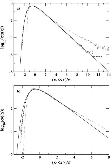
FIG. 3.: a) The PDF of the width-square for the sneppen model, sample sizes $T=50$ (dotted line) and $T=500$ (dashed line), the solid line is the FTG form. b) shows the PDF of the width-square for the 1/f-noise, sample sizes $T=64$ (dotted line), $T=4096$ (dashed line) and $T=32768$(dashed-dotted line), the solid line is the FTG form.

IV Discussion and Conclusion

We have studied the effects of correlations on extreme value statistics. Our aim has been to relate the Bramwell, Heldsworth and Pinton distribution [1, 2] to correlated extreme statistics. We have achieved this successfully for one specific system: the Sneppen depinning model.

We found that the extreme value statistics of the algebraically correlated avalanche signal is described by the BHP distribution. Furthermore we studied the width-square of the same signal and found this to be distributed according to the Fisher-Tippett-Gumbel distribution for uncorrelated extreme value statistics, though no extremes were explicitly involved for the width-square signal. This finding generalises a recent result by Antal, Droz, Györgyi and Rácz [4]. The BHP distribution and the FTG distribution are of similar functional form though they differ significantly for large fluctuations away from the mean, see [12].

Extreme value statistics for $1/f$ correlated signals were studied using renormalisation group (RG) techniques by Carpentier and Le Doussal [10]. They find that the correlations make the functional form change from the exponential decay of the uncorrelated FTG to the form $y\exp(-y)$ for fluctuations $y=x-\langle x\rangle\gg 0$ above the average (in the case of Maximum statistics). Note the $y\exp(-y)$ decay is identical to the asymptotic behaviour of the BHP distribution for large deviations above the average [2, 12]. Hence, the RG calculation by Carpentier and Le Doussal is an analytic indication of a relationship between the BHP distribution and extreme value statistics of logarithmically correlated variables. Our numerical study indicates a relationship in the case of algebraic correlations, at least in the specific example of the Sneppen model.

Signals with hierarchical correlations were considered in a recent preprint by Dean and Majumdar [11]. They find that correlations typically, though not always, alters the super-exponential $\exp(-\exp(y))$ found for $y<0$ in the uncorrelated FTG case, as well as in the BHP distribution. This result makes it clear that not all correlations make extreme value statistics follow the BHP distribution.

We conclude that correlated extreme value statistics may produce a limit distribution indistinguishable from the Bramwell-Holdsworth-Pinton distribution. More research is needed in order to determine the generality of this result.

V Acknowledgement

It is a pleasure to acknowledge stimulating discussion with our friends and colleagues at Imperial, especially K. Christensen, D. Hamon, M. Hall, S. Lise, M. Nicodemi and G. Pruessner. We are also indebted to G. Pruessner for pointing out Ref. [4]. HJJ greatly appreciates the exchange of general ideas concerning universal fluctuations with J. Lopez, P. Holdsworth and S. Bramwell. KD is supported by KTH.

^∗ Author to whom correspondence should be addressed. E-mail: h.jensen@ic.ac.uk

REFERENCES

- [1] S.T. Bramwell, P.C.W. Holdsworth and J.-F. Pinton , Nature 396, 552 (1998).
- [2] S.T. Bramwell et al. Phys. Rev. Lett. 84, 3744 (2000).
- [3] V. Aji and N. Goldenfeld, Phys. Rev. Lett. 86, 1007 (2001).
- [4] T. Antal, M. Droz G. Györgyi and Z. Rácz, arXiv:cond-mat/0105599
- [5] R.A. Fisher and L.H.C. Tippett, Cambridge Philos. Soc. 28, 180 (1928).
- [6] E.J. Gumbel, Statistics of Extremes, Columbia University Press, 1958); J. Galambos, The Asymtotic Theory of Extreme Order Statistics (R.E. Krieger Publ. Co., Malabar, Florida, 1987).
- [7] K. Sneppen, Phys. Rev. Lett. 69, 3539 (1992).
- [8] H.J. Jensen, Self-Organized Criticality, Cambridge Univeristy Press (1998).
- [9] W.H. Press, Comments Astrophys. Space Phys. 7, 103 (1978).
- [10] D. Carpentier and P. Le Doussal, Phys. Rev. E 63, 026110 (2100).
- [11] D.S. Dean and S.N. Majumdar, arXiv:cond-mat/0104028.
- [12] S.T. Bramwell, J.-Y. Fortin, P.C.W. Holdsworth, S. Peysson, B. Portelli, J.-F. Pinton, M. Sellitto, Phys. Rev. E63, 041106, (2001).