Susceptibility amplitude ratio
in the two-dimensional three-state Potts model

L. Shchur^a,b,c, P. Butera^b and B. Berche^c

^aLandau Institute for Theoretical Physics, 142432 Chernogolovka, Russia

^bInstituto Nazionale di Fisica Nucleare, Universitá Milano-Bicocca, Piazza delle Scienze 3, 20126, Milano, Italia

^cUniversité Henri Poincaré - Nancy I, Laboratoire de Physique des Matériaux, B.P. 239, 54506 Vandœuvre les Nancy Cedex, France

We analyze Monte Carlo simulation and series-expansion data for the susceptibility of the three-state Potts model in the critical region. The amplitudes of the susceptibility on the high- and the low-temperature sides of the critical point as extracted from the Monte Carlo data are in good agreement with those obtained from the series expansions and their (universal) ratio compares quite well with a recent quantum field theory prediction by Delfino and Cardy.

1 Introduction

The universal thermodynamic behaviour of a system in the vicinity of a critical point is characterized by a set of critical exponents and by universal combinations of critical amplitudes [1]. While the critical exponents are generally well studied, there are still few theoretical results on the universal combinations of critical amplitudes. Recently, some progress was achieved by Delfino and Cardy [2] (this reference shall be denoted as article I throughout our paper) for the two-dimensional $q$-state Potts model and some universal amplitude ratios were computed for $q=2,3$ and $4$ (see also  [3] for the most recent review on other results.)

It is commonly accepted that for a typical spin model, for instance the Ising model, there are only two independent length scales [4] in the critical region and thus there must be four universal relations [5] among the six following critical amplitudes: the amplitudes of specific heat in the ordered phase $A_{-}$ and in the symmetric phase $A_{+}$; the analogous amplitudes of the magnetic susceptibility $\Gamma_{-}$ and $\Gamma_{+}$; the amplitude of the magnetization when approaching the critical temperature from below,$B$; and the amplitude of the dependence of the magnetization on the magnetic field at the transition temperature, $D$. In the case of the two-dimensional Potts model with $q>2$, it is possible to define also a “transverse susceptibility” in the low temperature phase [7]. In terms of its critical amplitude $\Gamma_{T}$, a fifth universal ratio $\Gamma_{T}/\Gamma_{-}$ can be defined which is determined only by the behaviour in the LT phase.

The values of the ratio $\Gamma_{+}/\Gamma_{-}$ of the susceptibility critical amplitudes, were calculated in paper I with the results $37.699$, $13.848$ and $4.013$ for $q=2,3$ and $4$, respectively. The first value coincides with the well known exact result [6] in the four digits presented. In Ref. [7] Delfino, Barkema and Cardy performed a Monte Carlo (MC) test of the other predictions of paper I and found results for $\Gamma_{+}/\Gamma_{-}$ not consistent with their expectations in the $q=3$ case, while in the $q=4$ case their results were inconclusive. Actually the analysis of the data in the $q=4$ case is somewhat difficult due to the expected logarithmic corrections [8, 9, 10] to the power-like critical behaviour and the results [11] of a multi-parameter fit are still controversial (see, for instance Ref. [7]). On the other hand their analytical calculations for $\Gamma_{T}/\Gamma_{-}$ are in very good agreement with the numerical results reported in Ref. [7].

Here we present an analysis of the susceptibility of the $q=3$ Potts model by a MC simulation supported by extrapolations of the presently available LT and HT series expansions. The results of both procedure are completely consistent in the critical region window. The simplest extrapolation of the series expansions by Padé approximants yields the estimate $\Gamma_{+}/\Gamma_{-}=14.2(3)$, while a fit of the MC data leads to $\Gamma_{+}/\Gamma_{-}=14\pm 1$. Thus the agreement with the Delfino and Cardy prediction for $q=3$ is very good. Since also their estimate of the susceptibility ratio for $q=2$ is correct, our result gives us further confidence that even the prediction for the $q=4$ case might be correct. However, further numerical study of this case would still be welcome.

The text is organised as follows. In section 2 we define the model and present a few details of the series calculations and of the MC simulations. The data fitting procedure is discussed in the section 3 and the results are summarised and commented in section 4.

2 Model and Definitions

The Hamiltonian of the Potts model is

$$H=\sum_{<ij>}(1-\delta_{s_{i},s_{j}})+h\sum_{i}(1-\delta_{s_{i},0})$$ (1)

where $s_{i}$ is a site variable taking $q$ integer values between $0$ and $q-1$, and $h$ is an external magnetic field which stabilizes the state $0$.

The susceptibility is defined in terms of the free energy per site $f(\beta,h)$, where $\beta=1/T$ is the inverse temperature variable, starting with a finite system of $N$ sites and then taking the thermodynamic limit:

$$f(\beta,h)=\lim_{N\rightarrow\infty}-\frac{1}{N\beta}\log(Z_{N}(\beta,h))$$ (2)

with a partition function $Z_{N}$ defined according to

$$Z_{N}(\beta,h)=\sum_{conf}e^{-\beta H}.$$ (3)

The susceptibility at inverse temperature $\beta$ is thus

$$\chi(\beta)=\left.-\frac{1}{\beta}\frac{\partial^{2}f(\beta,h)}{\partial h^{2}}\right|_{h=0}\;.$$ (4)

2.1 Low-temperature and high-temperature expansions

The first few LT expansion coefficients can be very simply obtained by classifying the spin configurations with respect to their energy and multiplicity. In the LT variable $z=e^{-\beta}$ we have

$$\chi=(q-1)z^{4}+2(q-1)z^{6}+2(q-1)(q-2)z^{7}+...$$ (5)

It is by far less trivial to derive the very long LT expansions through $z^{47}$ tabulated in Ref. [12] for zero field in the $q=2,3$ and $4$ cases.

On the other hand, the presently available HT expansions for the susceptibility are still of moderate length. For general $q$, they reach  [13] the order $10$ in the HT variable

$$v=\frac{1-z}{1+(q-1)z}.$$

The first few terms of the expansion for $\chi$ are

$$\chi=1+4v+12v^{2}+36v^{3}+(76+12q)v^{4}+...$$

The HT series is however sufficient to compute accurately $\chi$ provided that one does not get too close to the critical point $\beta_{c}=\log(1+\sqrt{q})$. It should be noted that the HT expansion tabulated in Ref. [13] is conventionally normalized to 1 at infinite temperature and therefore it should be multiplied by the factor $\frac{q-1}{q^{2}}$ to get the correct amplitude.

We recall that the critical exponent is given by the exact formula

$$\gamma(q)=\frac{7\pi^{2}-8\mu\pi+4\mu^{2}}{6\pi(\pi-2\mu)}$$

with $\sqrt{q}=2\cos\mu$.

In terms of the HT series and of the known values of $\gamma$ and $\beta_{c}$, we can form, on the HT side of the critical point, the “HT effective amplitude” $\Gamma_{+}(\tau)=\tau^{\gamma}\chi(\tau)$. Here $\tau=1-\beta/\beta_{c}$ is the reduced inverse temperature. Similarly, we can construct a “LT effective amplitude” $\Gamma_{-}(\tau)=(-\tau)^{\gamma}\chi(\tau)$, on the LT side $\tau<0$ of the critical point. The critical amplitudes $\Gamma_{+}$ and $\Gamma_{-}$ are computed by extrapolating to the critical point the corresponding effective amplitudes. Since the HT series is not very long, the extrapolation can only be performed, in the most naive way, by Padé approximants, which cannot allow for the singular corrections to scaling. Therefore we should not expect an accuracy of the amplitude $\Gamma_{+}$ better than a few percent. The LT series is much longer, but we have preferred to use Padé approximants also in this case. We have used the highest order available approximants to extrapolate the effective amplitudes, namely the [5/5] approximant in the HT region, leading to $\Gamma_{+}=0.180(3)$ and the [22/22] approximant in the LT region, which gives $\Gamma_{-}=0.0127(1)$. In both cases we have checked the accuracy of the results by comparing these approximants with the lower order ones which are nearby in the Padé table. From this study we can conclude that $\Gamma_{+}/\Gamma_{-}=14.2(3)$. Since the largest contribution to the error comes from the determination of $\Gamma_{+}$, in order to improve the result, significantly longer HT series should be computed and the analysis should be performed by differential approximants, which can allow for the corrections to scaling.

2.2 Monte Carlo simulations

We adopt the Wolff algorithm [14] for studying square lattices of linear size $L$ with periodic boundary conditions. Starting from a typical ordered state, we let the system relax in $10^{4}$ steps measured by the number of flipped Wolff clusters. The averages are computed over $10^{5}$ steps. Our random numbers are produced by an exclusive-XOR combination of two shift-register generators with the taps (9689,471) and (4423,1393), which are known [15] to be safe for the Wolff algorithm.

The maximal system size $L=200$ we used is rather moderate for the current computer standards, but is quite sufficient for our purpose, as we will see.

During the simulations we have evaluated an order parameter $M(t)$ defined as follows

$$M=\frac{q\frac{N_{m}}{N}-1}{q-1}$$ (6)

where $N_{m}$ is the number of sites $i$ with $s_{i}=m$ at the time $t$ of the simulation [16], and $m\in[0...(q-1)]$ is the value of the majority of the spins at that time. This is like using the modulus of the magnetization in a MC simulations of Ising model.

Thus, the susceptibility in the LT phase is given by the fluctuations of the majority of the spins

$$k_{B}T\chi_{-}=\frac{1}{N}(<N_{m}^{2}>-<N_{m}>^{2})$$ (7)

while in the HT phase $\chi$ is given by fluctuations in all $q$ states,

$$k_{B}T\chi_{+}=\sum_{\mu=0}^{q-1}\frac{1}{qN}(<N_{\mu}^{2}>-<N_{\mu}>^{2}),$$ (8)

where $N_{i}$ is the number of sites $i$ with the spin in the state $\mu$. Properly allowing for the finite-size effects, this definition of the susceptibility gives, in both phases, an extremely good consistency with the series expansion data.

3 Data analysis

In this section we shall argue that system sizes such that $L\times L\approx 100\times 100$ sites are sufficiently large to reproduce the susceptibility behaviour of the infinite system in the range of the “critical temperature window”. Then we shall present a comparison of MC and series data. Finally, we shall discuss the fit to the data and comment on the quality of the results.

3.1 Critical region window

The critical region window $|\tau|\in[\tau_{fs},\tau_{corr}]$ is usually characterized [17, 7] as an interval between two (inverse reduced) temperatures $\tau_{fs}$ and $\tau_{corr}$ in which the finite system of size $L$ exhibits the critical behaviour of the infinite system. For instance, in the case of the susceptibility we should have

$$\chi\propto\Gamma_{\pm}|\tau|^{-\gamma}$$ (9)

where $\Gamma_{\pm}$ are the critical amplitudes in the HT phase (+) and in the LT phase (-), respectively, and $\gamma$ is the critical exponent. The “left-hand” boundary of the window $\tau_{fs}$ is the rather well defined temperature at which the correlation length $\xi\propto\tau^{-\nu}$ is of the order of the lattice size $L$, so that $\tau_{fs}\approx L^{-1/\nu}$. The “right-hand” limiting value of the critical window $\tau_{corr}$ is related to the corrections to scaling and could be defined as the temperature at which the deviation from the critical behaviour (9) due to the corrections to scaling reaches the level of e.g. $1\%$. Therefore the temperature $\tau_{corr}$ could be well identified knowing exactly the corrections to scaling as in the case of the Ising model [17, 18]. In the case of insufficient theoretical knowledge of the amplitudes of the correction terms, as is the case of the $3$-state Potts model, we can try to identify the “right-hand” temperature boundary $\tau_{corr}$ by plotting the MC data for the previously defined “effective amplitude”.

The MC results are shown in the Figure 1 together with the series expansion data which are denoted by thick solid lines. The series data compare well with the MC data also for size $L<80$ when $|\tau|>0.01$. The corrections to scaling are not small in the interval of the reduced temperature accessible by the Monte Carlo simulations.

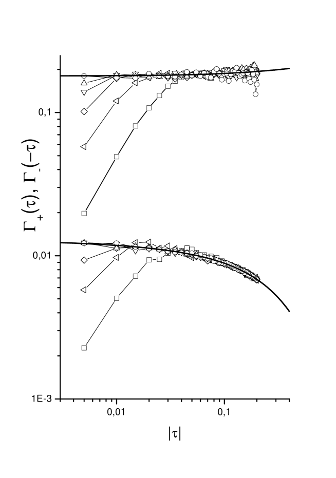
Figure 1: Finite-size behaviour of the effective amplitude of the susceptibility data in the critical region window. The data for lattice sizes $L=20,40,60,80,100$ and $200$ are denoted by squares, left-triangles, diamonds, down-triangles, up-triangles and circles, respectively. The high-temperature data correspond to the upper part and the low-temperature data to the lower part of the figure. The data generated from the high- and low-temperature series expansions are shown by thick solid lines.

3.2 Fit to the data

We have fitted the data taken in the critical window of the LT and HT phases to the following expression

$$\chi=\Gamma_{\pm}|\tau|^{-\gamma}(1+a_{\pm}|\tau|^{\Delta})+D_{\pm}$$ (10)

where $\gamma=13/9$ and $\Delta=y_{T,2}/y_{T,1}=2/3$ are known exactly [19], The value of $\Delta$ is supported by the series expansion analysis of Ref. [20], by a finite-size analysis [21] of the 3-state Potts quantum chain, and by a finite-size analysis of the transfer matrix results of Ref. [22]. The constant “background” terms $D_{\pm}$ are known to be important even for the Ising model [18], especially so in the LT phase. We have kept a single correction-to-scaling term $a_{\pm}|\tau|^{\Delta}$ in order to avoid introducing too many fitting parameters. However, we have also checked the stability under inclusion of further terms, e.g., $(1+a_{\pm}|\tau|^{\Delta}+b_{\pm}|\tau|+c_{\pm}|\tau|^{2\Delta})$ and found that $\Gamma_{\pm}$ varies only within the accuracy of the fit.

The results of the fit to the susceptibility data are shown in Table 1 for lattices sizes $L=20,40,60,80,100$ and $200$. The right-hand boundary of the critical window was chosen as $|\tau|=|(T-T_{c})/T|=0.2$ and the left-hand boundary according to the lattice size as $|\tau|>1/L^{1/\nu}$.

Table 1: Results of the fit to the MC susceptibility data in the critical region window. For comparison, we have also reported in the last line the results of a similar fit to the series expansion (SE) data.

$L$	$\Gamma_{-}$	$a_{-}$	$D_{-}$	$\Gamma_{+}$	$a_{+}$	$D_{+}$	$\Gamma_{+}/\Gamma_{-}$
20	0.01321(3)	-1.61(1)	0.0087(5)	0.2036(6)	-0.67(2)	0.37(1)	15.41(9)
40	0.01260(2)	-1.500(9)	0.0071(3)	0.1966(3)	-0.64(1)	0.448(8)	15.60(5)
60	0.01245(4)	-1.375(1)	0.0026(1)	0.1642(3)	0.90(2)	-0.228(6)	13.19(7)
80	0.01251(1)	-1.393(7)	0.0026(3)	0.1815(2)	0.14(1)	0.008(5)	14.51(3)
100	0.01250(1)	-1.41(6)	0.0037(3)	0.1728(16)	0.49(9)	-0.11(5)	13.82(16)
200	0.01273(1)	-1.509(6)	0.0070(2)	0.1741(2)	0.46(1)	-0.17(1)	13.68(3)
SE	0.012774(3)	-1.517(8)	0.0070(2)	0.1783(7)	0.24(2)	0.005(6)	13.96(7)

For comparison, we have also fitted in the same way the series expansion data, taking as critical window the interval $|\tau|\in[0.01:0.2]$ and assuming that the series expansion data become increasingly accurate for larger values of $|\tau|$. The error bars reflect the accuracy of the fit and do not allow for systematic deviations due to the fact that the critical window is far from the asymptotic limit when large corrections to scaling are present. The fit to the MC data shows stability and consistency with the series expansion data, listed in the last line of Table 1.

Very conservatively, we can conclude from our MC data and Padè approximation of series expansion that the ratio of the susceptibility amplitudes for the 3-state Potts model is $\Gamma_{+}/\Gamma_{-}=14\pm 1$. Thus, our results are completely consistent with the value $\Gamma_{+}/\Gamma_{-}=13.848$ calculated by Delfino and Cardy [2].

An additional check of the results is obtained by studying the ratio $r^{(SE)}(\tau)$ of the HT and the LT effective amplitudes of the susceptibility, as computed from series expansions $r^{(SE)}(|\tau|)=\Gamma_{+}(\tau)/\Gamma_{-}(-\tau)$. We can expect the following behaviour of this ratio

$$r^{(SE)}(|\tau|)=\frac{\Gamma_{+}}{\Gamma_{-}}\left(1+a_{1}|\tau|^{\Delta}+a_{2}|\tau|+a_{3}|\tau|^{2\Delta}+...\right)$$ (11)

as $\tau\rightarrow 0+$.

A three-parameter ($\frac{\Gamma_{+}}{\Gamma_{-}}$, $a_{1}$, and $a_{2}$) fit of $r^{(SE)}(|\tau|)$ in the temperature window $[0.01:0.1]$ gives $\frac{\Gamma_{+}}{\Gamma_{-}}=14.2(5)$.

In the case of the Ising model ($q=2$ Potts model), a similar fit of the same ratio $r^{(SE)}(|\tau|)$ to the form

$$r^{(SE)}(|\tau|)=\frac{\Gamma_{+}}{\Gamma_{-}}\left(1+a_{1}|\tau|+a_{2}|\tau|\log|\tau|\right)$$ (12)

leads to a value of the critical amplitude ratio $\frac{\Gamma_{+}}{\Gamma_{-}}=39\pm 2$ which is consistent with the exact value $37.69365...$. The large error bars are due to the fact that we have used series expansions of the same length as for the 3-state Potts model in order to test under similar conditions the accuracy of the method. Of course, much better results could obtained fully using the much longer series expansions which are available for the 2d Ising model [23].

4 Summary of the results and conclusions

The values of the suceptibility critical amplitude ratio for the Potts model with $q=2,3$ and $4$ were calculated by Delfino and Cardy [2] using the two-kink approximation of the exact scattering theory for the Potts model [24]. The value $37.699$ thus obtained for the ratio in the $q=2$ case (Ising model) agrees well with the exactly known value. However the same authors and Barkema were unable to confirm numerically [7] their theoretical results: $13.848$ for the $q=3$ Potts model and $4.013$ for the 4-state Potts model. The discussion of the latter case is beyond present paper. However by analysing our MC data and the existing series expansions, we find that the critical amplitude ratio for the 3-state Potts model can be very safely identified with the estimate $14\pm 1$, quite consistently with the prediction by Delfino and Cardy.

What is the main difference between the analysis of Ref. [7] and that presented here? First, we calculate the amplitudes separately in both the LT and the HT phases by fitting the temperature behaviour of the susceptibilities. It is also important that the value of susceptibility was computed by not less than $10^{5}$ Wolff MonteCarlo steps at each value of temperature. Indeed the fit to the susceptibility becomes unstable for smaller statistics. Next, we have computed the amplitude ratio as a function of temperature defined in the same way in both phases. This is not the case for the analysis in Ref. [7], where the corresponding temperatures in the two phases are shifted by a factor proportional to the ratio of the correlation lengths.

Since two out of the three $\Gamma_{+}/\Gamma_{-}$ ratio values computed by Delfino and Cardy agree well, either with the known exact result for the Ising case, or with our MC and series expansion data for $q=3$, little doubt remains, in our opinion, that also their prediction for the 4-state Potts model may be correct. We wish to quote here a MC analysis of the 4-state Potts model by Caselle et al. where an estimate consistent with the Delfino and Cardy prediction is obtained. However Delfino et al. [7] did not found this analysis completely satisfactory and therefore the susceptibility ratio prediction for $q=4$ is still waiting for further numerical verifications.

5 Acknowledgements

LNS is grateful to the Theoretical Physics group of the Milano-Bicocca University and to the Statistical Physics group of the University Henri Poincaré Nancy-I for their kind hospitality. Financial support from the twin research program between the Landau Institute and the Ecole Normale Supérieure de Paris as well as financial support from the CARIPLO Foundation and Landau Network—Centro Volta, and Russian Foundation for Basic Research under project 99-07-18412 are also acknowledged.

References

- [1] V. Privman, P.C. Hohenberg, A. Aharony, in Phase Transitions and Critical Phenomena, Vol. 14, edited by C. Domb and J.L. Lebowitz (Academic, New York, 1991).
- [2] G. Delfino and J.L. Cardy, Nucl. Phys. B 519 [FS] (1998) 551.
- [3] G. Mussardo, hep-th/0010164.
- [4] D. Stauffer, M. Ferer, and M. Wortis, Phys. Rev. Lett. 29 (1972) 345.
- [5] A. Aharony and P.C. Hohenberg, Phys. Rev. B 13 (1976) 3081.
- [6] T.T. Wu, B.M. McCoy, C.A. Tracy and E. Barouch, Phys. Rev. B 13 (1976) 316.
- [7] G. Delfino, G.T. Barkema, and J.L. Cardy, Nucl. Phys. B 565 (2000) 521.
- [8] N. Nauenberg and D.J. Scalapino, Phys. Rev. Lett. 44 (1980) 837.
- [9] J. L. Cardy, N. Nauenberg and D.J. Scalapino, Phys. Rev B 22 (1980) 2560.
- [10] J. Salas and A. Sokal, J. Stat. Phys. 88 (1997) 567.
- [11] M. Caselle, R. Tateo, S. Vinti, Nucl. Phys. B 562 (1999) 549.
- [12] K.M. Briggs, I.G. Enting, and A.J. Guttmann, J. Phys. A 27 (1994) 1503.
- [13] G. Shreider and J.D. Reger, J. Phys. A. 27 (1994) 1071.
- [14] U. Wolff, Phys. Rev. Lett. 62 (1989) 361.
- [15] L.N. Shchur, Comp. Phys. Comm., 121-122 (1999) 83.
- [16] K. Binder, J. Stat. Phys, 24 (1981) 69.
- [17] A.L. Talapov and L.N. Shchur, J. Phys.: Cond. Matt., 6 (1994) 8295.
- [18] L.N. Shchur and O.A. Vasilyev, to be published in Phys. Rev. E
- [19] B. Nienhuis, J. Phys. A, 15 (1982) 199.
- [20] J. Adler and V. Privman, J. Phys. A, 15 (1982) L417.
- [21] G. von Gehlen, V. Rittenberg, and T. Vescan, J. Phys. A, 20 (1987) 2577.
- [22] S.L.A. de Queiroz, J. Phys. A, 33 (2000) 721.
- [23] W. P. Orrick, B. Nickel, A. J. Guttmann, and J. H. H. Perk, Phys. Rev. Lett. 86 (2001) 4120; J. Stat. Phys. 102 (2001) 795.
- [24] L. Chim and A.B. Zamolodchikov, Int. J. Mod. Phys. A, 7 (1992) 5317.