Phonon drag in ballistic quantum wires

Abstract

The acoustic phonon–mediated drag contribution to the drag current created in the ballistic transport regime in a one–dimensional nanowire by phonons generated by a current–carrying ballistic channel in a nearby nanowire is calculated. The threshold of the phonon–mediated drag current with respect to bias or gate voltage is predicted.

]

I Introduction

The purpose of the present paper is to study the phonon contribution to the drag current in the course of ballistic (collisionless) electron transport in a nanowire due to a ballistic driving current in an adjacent parallel nanowire. Early the possibility of the Coulomb drag (CD) effect in the ballistic regime in quantum wires has been demonstrated by Gurevich, Pevzner and Fenton [1] and has been experimentally observed by Debray et al. [2], [3]. Using the approach of [4], [5] we consider two parallel ballistic quantum channels that are connected to two thermal reservoirs, each being in an independent equilibrium state. As was recently shown, although most of the heat from a current through the channel is generated in the reservoirs [6] part of the heat is generated by the current carrying nanostructure itself [7] via emission of phonons. Electrons penetrating into a biased (drive) wire from the leads are characterized by different chemical potentials, the situation is nonequilibrium and the phonons are generated by the drive wire.

There has been done much work on the phonon contribution to the drag current in a two-dimensional electron gas situation [8]. However, we are not aware of any work on the phonon drag in ballistic quantum wires. The electrons in the nearby (drag) nanowire being initially in an equilibrium absorb the ballistic phonons emitted by the drive wire and the phonon drag current is created. Similar to the CD situation here we encounter that in the course of backscattering of electrons in the drive wire the phonons with quasimomentum $\hbar q_{z}=2p_{n}$ are generated that in their turn are absorbed by the drag wire. The contribution to the current of two subbands $\varepsilon_{l}+p^{2}/2m$ in the drive wire and $\varepsilon_{n}+p^{2}/2m$ in the drag wire vanishes unless

$$eV/2\,>\,|\varepsilon_{l}-\varepsilon_{n}|$$

again similar to the CD case [9]. However, in the phonon drag we encounter the threshold

$$eV/2\,>\,sp_{n}.$$

Indeed, the energy-momentum conservation leads to

$$\hbar\omega_{\bf q}=\varepsilon_{p+\hbar q_{z}}-\varepsilon_{p}$$

that can be rewritten using $q\cos{\theta_{q}}=q_{z}$ as

$$|\cos{\theta_{q}}|={2ms\over{|p+\hbar q_{z}|-p}}\,<\,1$$

Now taking into account that $|p+\hbar q_{z}|,p$ should be in the vicinity of $p_{n}\pm\,eV/2v_{n}$ we get the threshold condition $eV/2\,>\,sp_{n}$.

II Phonon spatial distribution

We assume that the length of the nanowires $L$ is much greater than the transverse dimensions of the wires. Therefore the spatial distribution of the emitted by the drive wire ballistic (nonequilibrium) phonons with wave vector ${\bf q}$, $\delta N_{\bf q}({\bf r})$ given by the stationary Boltzmann equation

$${\bf s}\nabla\delta N_{\bf q}={\cal R}$$ (1)

where ${\bf s}={\partial\omega_{\bf q}}/\partial{\bf q}$ is the group sound velocity, $\hbar\omega_{\bf q}$ is the phonon energy, ${\cal R}$ is the collision operator describing phonon generation, can be rewritten in the form

$$(\partial_{x}+\alpha\partial_{y})\delta N_{\bf q}(x,y)={{\cal R}\over{s_{x}}},\;\;\alpha\equiv\,{s_{y}\over{s_{x}}}=\tan{\varphi_{q}}.$$ (2)

We assume that the spatial distribution of the generated phonons depends only on the transverse coordinates $x,y$. The collision operator ${\cal R}$ can be written as

$${\cal R}={1\over{{\cal V}}}\sum_{ll^{\prime}}\int{2Ldk\over{2\pi\hbar}}W_{\bf q}\left|C_{ll^{\prime}}({\bf q}_{\perp})\right|^{2}$$ (3)

$$\times\left[f_{l,k+\hbar q_{z}}(1-f_{l^{\prime}k})(N_{\bf q}^{eq}+1)\right.$$ (4)

$$\left.-f_{l^{\prime},k}(1-f_{l,k+\hbar q_{z}})N_{\bf q}^{eq}\right]$$ (5)

$$\times\delta(\varepsilon_{l,k+\hbar q_{z}}-\varepsilon_{l^{\prime},k}-\hbar\omega_{\bf q}),$$ (6)

where ${\cal V}$ is the volume of the channel, $C_{ll^{\prime}}(\bf q)=<l|e^{i{\bf qr}_{\perp}}|l^{\prime}>$ is the matrix element for phonon induced transitions, $W_{\bf q}$ is the electron–phonon coupling constant that for the deformation potential interaction is $W_{\bf q}=\pi\Lambda^{2}q^{2}/\rho\omega_{\bf q}$, where $\Lambda$ is the deformation potential constant, $\rho$ is the mass density.

According to approach in [4], [5] we express the distribution functions in Eq.(3) as the Fermi functions $f^{F}(\varepsilon_{lp}-\mu^{(R,L)})$ with shifted chemical potentials $\mu^{(R,L)}=\mu\pm\,eV/2$, $\mu$ is the quasi Fermi level that depends on the gate voltage and $V$ is the bias voltage.

What is concerning the collision operator spatial dependence we assume that it has nonzero values only within the nanowire.

Restricting ourselves by the case $T=0$ we consider only the spontaneous term in Eq.(3) since there is no equilibrium phonons $N_{\bf q}^{eq}=0$.

$${\cal R}_{sp}={1\over{{\cal V}}}\sum_{ll^{\prime}}\int{2Ldk\over{2\pi\hbar}}W_{\bf q}\left|C_{ll^{\prime}}({\bf q}_{\perp})\right|^{2}$$ (7)

$$\times[f_{l,k+\hbar q_{z}}\times(1-f_{l^{\prime}k})-f_{l,k+\hbar q_{z}}^{eq}(1-f_{l^{\prime}k}^{eq})]$$ (8)

$$\times\delta(\varepsilon_{l,k+\hbar q_{z}}-\varepsilon_{l^{\prime},k}-\hbar\omega_{\bf q})$$ (9)

Here in Eq.(7) we take into account explicitly that phonons are generated by the nonequilibrium electrons.

We assume the channels have uniform cross sections, the origin of the system of reference being in the center of the current–carrying (drive) wire, the drag wire being shifted along the $x$ axis by the distance $D$. Therefore we need the solution of Eq.(2) only for $s_{x}\,>0$.

The solution of the Eq.(2) depends on the cross section geometry of the wire. Assuming, for simplicity, that the cross section of the wire is a circle (it is worth noting that the result does not change significantly for other geometries of the cross section) of the radius $R$ we get for the coordinates outside the wire cross section

$$\delta N_{\bf q}={2{\cal R}_{sp}\over{s_{x}(1+\alpha^{2})}}\sqrt{R^{2}(1+\alpha^{2})-(y-\alpha x)^{2}}$$ (10)

$$\times\Theta[R^{2}(1+\alpha^{2})-(y-\alpha x)^{2}].$$ (11)

The geometrical interpretation of this solution is physically transparent (see Fig. 1): let us draw a line through the center of the cross section of the wire having the angle $\varphi_{s}$, $\tan\varphi_{s}=\alpha$ with $x$ axis. Now consider a line parallel to the already drawn one and crossing the cross section of the wire. The distance $|AC|$ from the point $x,y$ outside the cross section of the wire and lying on the second line to the first line is $|y-\alpha x|\cos{\varphi_{s}}=|y-\alpha x|/\sqrt{1+\alpha^{2}}$. The $\Theta$-function in Eq.(10) states that if this distance is smaller than the radius R (i.e. the second line does cross the cross section of the wire) the result is proportional to the length of the chord cut from the second line by the cross section, otherwise the result is zero.

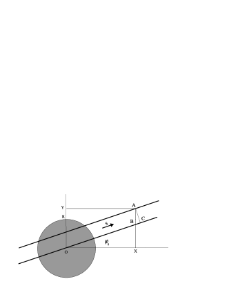
FIG. 1.: Schematic representation of the cross section of the drive wire (shaded region) and the direction of phonons’ propagation.

The similar interpretation is valid for the other geometries of the wire cross section.

III Phonon drag contribution to the drag current

Now in the drag wire due to an electron-phonon interaction we have $f_{n}=f_{n}^{(F)}+\Delta f_{n}$ with $\Delta f_{n}$ satisfying the equation [1]

$$v{\partial\Delta f_{n}\over{\partial z}}=I[f_{n}],$$ (12)

where $v=\partial\varepsilon_{n}/\partial p$ is the electron velocity, $I[f]$ is the electron–phonon collision term. For $p>0\,(p<0)$ respectively the solution of this equation is

$$\Delta f_{n}(z)=(z\pm L/2){1\over{v}}I[f_{n}].$$ (13)

The boundary condition is $\Delta f[p>0\,(p<0)]=0$ at $z=\mp L/2$. The current then is given by

$$J=e{1\over{\cal V}}\sum_{n,p}\int d{\cal A}v\Delta f_{n}$$ (14)

$$=e\sum_{n}\int{dxdy\over{{\cal A}}}\int_{0}^{\infty}{2Ldp\over{2\pi\hbar}}I[f_{n}].$$ (15)

Here the integration is over the cross section ${\cal A}$ of the drag wire. The electron phonon collision term is

$$I[f_{n}]=\sum_{n^{\prime}}\int{dp^{\prime}\over{2\pi\hbar}}\int{d{\bf q}_{\perp}\over{(2\pi)^{2}}}W_{\bf q}\left|C_{nn^{\prime}}({\bf q}_{\perp})\right|^{2}$$ (16)

$$\times\{\left[f_{n^{\prime}p^{\prime}}(1-f_{np})(N_{p^{\prime}-p}+1)\right.$$ (17)

$$-\left.f_{np}(1-f_{n^{\prime}p^{\prime}})N_{p^{\prime}-p}\right]$$ (18)

$$\times\delta(\varepsilon_{np}-\varepsilon_{n^{\prime}p^{\prime}}+\hbar\omega_{p^{\prime}-p})$$ (19)

$$+\left[f_{n^{\prime}p^{\prime}}(1-f_{np})N_{p-p^{\prime}}\right.$$ (20)

$$-\left.f_{np}(1-f_{n^{\prime}p^{\prime}})(N_{p-p^{\prime}}+1)\right]$$ (21)

$$\times\delta(\varepsilon_{np}-\varepsilon_{n^{\prime}p^{\prime}}-\hbar\omega_{p-p^{\prime}})\}.$$ (22)

In $N_{\bf q}$ and $\omega_{\bf q}$ we indicate explicitly only the longitudinal component of quasimomenta of phonons. The first and second term in Eq.(16) describes the $N_{p^{\prime}-p}$ phonon generation in the electron transition $\varepsilon_{n^{\prime}p^{\prime}}\rightarrow\varepsilon_{np}$ and absorption of the phonon $N_{p^{\prime}-p}$ via the electron transition $\varepsilon_{np}\rightarrow\varepsilon_{n^{\prime}p^{\prime}}$ respectively. The third and forth terms describe absorption of the phonon $N_{p-p^{\prime}}$ ($\varepsilon_{n^{\prime}p^{\prime}}\rightarrow\varepsilon_{np}$) and generation ($\varepsilon_{np}\rightarrow\varepsilon_{n^{\prime}p^{\prime}}$) of the phonon $N_{p-p^{\prime}}$. For the current induced in the drag wire by the phonons emitted by the drive wire we get

$$J=e\sum_{n,n^{\prime}}\int{dxdy\over{{\cal A}}}\int_{0}^{\infty}{2Ldp\over{2\pi\hbar}}\int_{-\infty}^{\infty}{dp^{\prime}\over{2\pi\hbar}}$$ (23)

$$\int\,{d{\bf q}_{\perp}\over{(2\pi)^{2}}}W_{\bf q}\left|C_{nn^{\prime}}({\bf q}_{\perp})\right|^{2}[f_{n^{\prime}p^{\prime}}-f_{np}]$$ (24)

$$\times\left\{\delta N_{p^{\prime}-p}\delta(\varepsilon_{np}-\varepsilon_{n^{\prime}p^{\prime}}+\hbar\omega_{p^{\prime}-p})\right.$$ (25)

$$+\delta N_{p-p^{\prime}}\left.\delta(\varepsilon_{np}-\varepsilon_{n^{\prime}p^{\prime}}-\hbar\omega_{p-p^{\prime}})\right\}.$$ (26)

Here the distribution functions $f_{(n,n^{\prime})}$ are equilibrium Fermi functions $f^{F}(\varepsilon_{np}-\mu)$. Assuming that the angle dependence is involved only through the phonon distribution we can take an average over the cross section of the drag wire and integrate over the angles $\varphi_{q}$

$$\int{dxdy\over{\pi R^{2}}}\int{q_{\perp}dq_{\perp}\over{(2\pi)^{2}}}d\varphi_{q}\Delta N_{\bf q}={2R\over{(2\pi)^{2}s\pi}}$$ (27)

$$\times\int{qdq_{\perp}}\,{\cal R}_{sp}\int_{0}^{1}\rho d\rho\int_{0}^{2\pi}d\varphi\int_{-\pi/2}^{\pi/2}d\varphi_{q}$$ (28)

$$\times\sqrt{1-\left(\rho\sin{\varphi}-{D\over{R}}\sin{\varphi_{q}}\right)^{2}}.$$ (29)

Since $D/R\gg\,1$ we see that only small angles contribute to the integral

$${R\over{D}}(\rho\sin{\varphi}-1)<\sin{\varphi_{q}}\simeq\,\varphi_{q}\,<\,{R\over{D}}(\rho\sin{\varphi}+1).$$

Therefore, the result

$$\int_{-{R\over{D}}(1-\rho\sin{\varphi})}^{{R\over{D}}(\rho\sin{\varphi}+1)}d\varphi_{q}\sqrt{1-\left(\rho\sin{\varphi}-{D\over{R}}{\varphi_{q}}\right)^{2}}={\pi\over{2}}{R\over{D}}$$

is proportional to the (solid) angle $R/D$ of the cross section of the drag wire relative to the drive wire. This factor simply reflects the fact that phonons emitted by the drive wire should penetrate the drag wire.

$$\int{dxdy\over{\pi R^{2}}}\int{q_{\perp}dq_{\perp}\over{(2\pi)^{2}}}d\varphi_{q}\Delta N_{\bf q}=$$ (30)

$${1\over{4\pi}}{R\over{s}}{R\over{D}}\int{qdq_{\perp}}\,{\cal R}_{sp}.$$ (31)

Inserting this expression in the expression for the current and taking into account energy conservation laws

$$\delta(\varepsilon_{np}-\varepsilon_{n^{\prime}p^{\prime}}+\hbar\omega_{p^{\prime}-p})$$ (32)

$$\times\delta(\varepsilon_{lk+p^{\prime}-p}-\varepsilon_{l^{\prime}k}-\hbar\omega_{p^{\prime}-p})=$$ (33)

$$={m\over{\hbar s|p-p^{\prime}|}}\delta\left(k-p-{m\delta\over{p-p^{\prime}}}\right)$$ (34)

$$\times\delta\left(q-{\varepsilon_{n^{\prime}p^{\prime}}-\varepsilon_{np}\over{\hbar s}}\right),$$ (35)

that allows the integration over $k$ we get

$$J=e{Lm\pi\Lambda^{4}\over{8D\rho^{2}(\pi s\hbar)^{4}}}\sum_{nn^{\prime}ll^{\prime}}\int_{0}^{\infty}dp\int_{-\infty}^{\infty}dp^{\prime}$$ (36)

$$\int_{|p-p^{\prime}|/\hbar}^{\infty}{q^{4}dq\over{\sqrt{q^{2}-(p-p^{\prime}/\hbar)^{2}}}}\left|C_{nn^{\prime}}({\bf q}_{\perp})\right|^{2}$$ (37)

$$\times\left|C_{ll^{\prime}}({\bf q}_{\perp})\right|^{2}[f_{n^{\prime}p^{\prime}}-f_{np}]{1\over{|p-p^{\prime}|}}$$ (38)

$$\times\{f_{lp^{\prime}+m\delta/(p-p^{\prime})}(1-f_{l^{\prime}p+m\delta/(p-p^{\prime})})$$ (39)

$$\times\delta\left(q-{\varepsilon_{n^{\prime}p^{\prime}}-\varepsilon_{np}\over{\hbar s}}\right)$$ (40)

$$+f_{lp+m\gamma/(p-p^{\prime})}(1-f_{l^{\prime}p^{\prime}+m\gamma/(p-p^{\prime})})$$ (41)

$$\times\delta\left(q-{\varepsilon_{np}-\varepsilon_{n^{\prime}p^{\prime}}\over{\hbar s}}\right)\},$$ (42)

Here $\delta$ and $\gamma$ stand for $\delta=\varepsilon_{n}+\varepsilon_{l}-\varepsilon_{n^{\prime}}-\varepsilon_{l^{\prime}}$ $\gamma=\varepsilon_{n}+\varepsilon_{l^{\prime}}-\varepsilon_{n^{\prime}}-\varepsilon_{l}$. Integrating over $q$ we get

$$J=e{Lm\Lambda^{4}\over{8D\rho^{2}\pi^{3}(s\hbar)^{7}}}\sum_{nn^{\prime}ll^{\prime}}\int_{0}^{\infty}dp\int_{-\infty}^{\infty}dp^{\prime}$$ (43)

$$\times[f_{n^{\prime}p^{\prime}}-f_{np}]{P_{nn^{\prime}ll^{\prime}}(p,p^{\prime})\over{|p-p^{\prime}|}}$$ (44)

$$\times\left\{f_{lp^{\prime}+m\delta/(p-p^{\prime})}(1-f_{l^{\prime}p+m\delta/(p-p^{\prime})})\right.$$ (45)

$$\Theta\left(\varepsilon_{n^{\prime}p^{\prime}}-\varepsilon_{np}-s|p-p^{\prime}|\right)$$ (46)

$$+f_{lp+m\gamma/(p-p^{\prime})}(1-f_{l^{\prime}p^{\prime}+m\gamma/(p-p^{\prime})})$$ (47)

$$\left.\Theta\left(\varepsilon_{np}-\varepsilon_{n^{\prime}p^{\prime}}-s|p-p^{\prime}|\right)\right\},$$ (48)

where we introduced notation

$$P_{nn^{\prime}ll^{\prime}}(p,p^{\prime})={(\varepsilon_{n^{\prime}p^{\prime}}-\varepsilon_{np})^{4}\over{\phi_{n,n^{\prime}}(p,p^{\prime})}}$$ (49)

$$\times\left|C_{nn^{\prime}}\left({1\over{\hbar s}}\phi_{n,n^{\prime}}(p,p^{\prime})\right)\right|^{2}$$ (50)

$$\times\left|C_{ll^{\prime}}\left({1\over{\hbar s}}\phi_{n,n^{\prime}}(p,p^{\prime})\right)\right|^{2},$$ (51)

where

$$\phi_{n,n^{\prime}}(p,p^{\prime})=\sqrt{(\varepsilon_{n^{\prime}p^{\prime}}-\varepsilon_{np})^{2}-s^{2}(p-p^{\prime})^{2}}.$$ (52)

Let us consider the case when $n=n^{\prime}$ and $l=l^{\prime}$. Then $\delta=\gamma=0$.

Now taking into account that the phonons are emitted by the electrons having negative initial momentum [the nonequilibrium functions $f_{l,p}$ are Fermi functions with shifted by $eV/2>0$ chemical potentials, i.e. $f_{lp}=f^{L}_{lp}$ for $p>0$ and $f_{lp}=f^{R}_{lp}$ for $p<0$ ($f^{L}=f^{F}(\varepsilon-[\mu-eV/2])$, $f^{R}=f^{F}(\varepsilon-[\mu+eV/2])$)] and that the integrals vanish unless the Fermi functions $f$ and $1-f$ under the integral overlap one conclude that $p^{\prime}$ satisfying $-\infty\,<p^{\prime}<\,-p-2p_{s}$, $p_{s}=ms$, contribute to the current. To avoid further confusion about the drag current direction note that we consider $eV>0$ and therefore the first term in the right hand side of Eq.(43) survives, otherwise if $eV<0$ only the second term in this equation would contribute to the current and due to $f_{np^{\prime}}-f_{np}$ the current would change the sign. We have after transformation $p^{\prime}\rightarrow\,-p^{\prime}$

$$J=e{Lm\Lambda^{4}\over{8D\rho^{2}\pi^{3}(s\hbar)^{7}}}\sum_{nl}\int_{0}^{\infty}dp\int_{-\infty}^{-p-2p_{s}}dp^{\prime}$$ (53)

$$\times[f_{np^{\prime}}-f_{np}]{P_{nl}(p,p^{\prime})\over{|p-p^{\prime}|}}f_{lp^{\prime}}^{R}(1-f_{lp}^{L})$$ (54)

$$=e{Lm\Lambda^{4}\over{8D\rho^{2}\pi^{3}(s\hbar)^{7}}}\sum_{nl}\int_{0}^{\infty}dp\int_{p+2p_{s}}^{\infty}dp^{\prime}$$ (55)

$$\times[\Theta(p_{n}-p^{\prime})-\Theta(p_{n}-p)]$$ (56)

$$\times{P_{nl}(p,-p^{\prime})\over{p+p^{\prime}}}\Theta(p-p_{l}^{-})\Theta(p_{l}^{+}-p^{\prime}),$$ (57)

where

$$p_{n}=\sqrt{2m(\mu-\varepsilon_{n})},\;\;p_{n}^{\pm}=\sqrt{2m(\mu-\varepsilon_{n}\pm eV/2)}.$$

We get the nonzero result only if

$$p_{l}^{+}-p_{l}^{-}\,>2p_{s},\;\;\;p_{l}^{-}<p_{n}<p_{l}^{+}$$ (58)

The last inequality is equivalent to

$$eV/2\,>\,|\varepsilon_{n}-\varepsilon_{l}|=|\varepsilon_{nl}|.$$

Assuming $eV/2\ll\,p_{n}^{2}/2m$, $|\varepsilon_{nl}|\ll\,p_{n}^{2}/2m$ we have nonzero result only if

$$eV/2\,>\,\mbox{max}\{sp_{n},|\varepsilon_{nl}|\}.$$

Let us put $\varepsilon_{nl}=0$, we obtain for $eV/2\,<\,2sp_{n}$ ($\alpha\equiv\,eV/4sp_{n}$), i.e. $1/2\,<\alpha\,<1$

$$J=J_{0}\sum_{n}\left({v_{n}\over{s}}\right)^{2}\int_{1}^{2\alpha}dt(2\alpha-t)T(t)$$ (59)

and for $eV/2\,>\,2sp_{n}$ ($\alpha\,>1$)

$$J=J_{0}\sum_{n}\left({v_{n}\over{s}}\right)^{2}\left\{\int_{1}^{\alpha}dt\,t\right.$$ (60)

$$+\left.\int_{\alpha}^{2\alpha}dt(2\alpha-t)\right\}T(t).$$ (61)

$$J_{0}=-e{2Lm^{5}\Lambda^{4}\over{\pi^{3}D\rho^{2}\hbar^{7}}}$$ (62)

$$T(t)={t^{4}\over{\sqrt{t^{2}-1}}}\left|C_{nn}\left({2p_{n}\over{\hbar}}\sqrt{t^{2}-1}\right)\right|^{2}$$ (63)

$$\times\left|C_{ll}\left({2p_{n}\over{\hbar}}\sqrt{t^{2}-1}\right)\right|^{2}.$$ (64)

Assuming the following model dependence for $C_{nn}$

$$|C_{nn}(q)|^{2}={1\over{(1+qR)^{2}}}$$ (65)

we plot in Fig. 2 the drag current versus the voltage applied across the drive nanowire for different $p_{n}$ values $p_{1}R/\hbar=3.33$ and $p_{2}R/\hbar=5$.

FIG. 2.: Drive voltage dependence of the phonon contribution to the drag current for different values of $p_{n}$.

Near the threshold $\alpha-1/2\ll\,1$ we get, assuming $2\alpha-1\ll\,(\hbar/2p_{n}R)^{2}$ so that the argument of the function $C_{nn}$ is small and $C_{nn}\sim\,1$

$$J=-e{4\sqrt{2}Lm^{5}\Lambda^{4}\over{3D\rho^{2}\pi^{3}\hbar^{7}}}\left({v_{n}\over{s}}\right)^{2}\left({eV\over{2sp_{n}}}-1\right)^{3/2},$$ (66)

$$1<{eV\over{2sp_{n}}}(<2)$$ (67)

i.e. at the threshold the current increases nonlinearly with the applied voltage. This dependence is illustrated by the small inlet in Fig. 2 since it can be noted only in very small vicinity near the threshold.

The second derivative of the current with respect to the bias voltage diverges as

$${d^{2}J\over{dV^{2}}}\sim{1\over{\sqrt{eV/2sp_{n}-1}}}$$

at the threshold for any new subband $n$, this fact can be instrumental for the experimental investigation.

Assuming the following parameters $eV/4sp_{n}\geq\,1$, (for $s\simeq\,3\cdot\,10^{5}\,\,$ cm/s, $\hbar/p_{n}\simeq\,0.5\cdot\,10^{-6}\,\,$ cm this means voltages $V\sim$ mV), $p_{n}R/\hbar\simeq\,1$, $L\simeq\,2\,\,\mu$m, $D\sim\,0.1\cdot\mu$m, $\Lambda\sim\,8\,$ eV, $m=0.07m_{0}$ we get the following estimation for the contribution of any subband to the phonon-mediated drag current

$$J\sim\,3\cdot\,10^{-12}\;A$$

IV Conclusion

We note two essential differences between the phonon drag and the Coulomb drag. First, it is the existence of the threshold $eV/2\,>\,sp_{n}$ (that can be achieved changing either the bias voltage or the gate voltage). Second, the weak dependence on the distance $D$ between the centers of the drive and drag wires rather than the exponential one in the CD case. On the other hand, note, that the distance dependence of the phonon drag current in our case is stronger than the distance dependence of the phonon drag between two 2DEG layers [8].

The coupling coefficient for the piezoelectric coupling for GaAs having the cubic ${\bf T_{d}}$ symmetry can be written as

$$W_{\bf q}={\pi\over{\rho\omega_{\bf q}}}\left[{4\pi e\beta\over{\epsilon}}\right]^{2}\left(F(\theta_{q},\varphi_{q})\right)^{2},$$

where $F(\theta_{q},\varphi_{q})$ is a function of angles. The estimations for GaAs ($\beta=10^{5}$ SGS units, $\epsilon=12$, $\Lambda=8$ eV, $\rho=5$ g/cm³, $s=3\times\,10^{5}$ cm/s) shows that the piezoelectric interaction is the dominating one for frequencies $\omega_{\bf q}\leq\,10^{11}\;$ s^-1.

Frequencies of transmitted phonons in the phonon drag are $\omega_{q}\,>\,2s/(\hbar/p_{n})$, i.e. are greater than $10^{12}$ s^-1. Therefore, the contribution of the piezoelectric coupling is smaller than the considered deformation potential coupling.

And finally, one can express the drag current also as an integral over the transferred phonon momentum $q_{z}$ in an electron-electron interaction. We get a physically transparent result

$$J=e{1\over{\cal V}^{2}}\int_{sw}\,{dxdy\over{{\cal A}}}\sum_{n,l,{\bf q},q_{z}>0}\left|W_{\bf q}\right|^{2}$$ (68)

$$\times\left|C_{ll}({\bf q}_{\perp})\right|^{2}{2q\over{sq_{\perp}}}\sqrt{R^{2}-s^{2}\left(yq_{x}/q-xq_{y}/q\right)^{2}}$$ (69)

$$\times\left|C_{nn}({\bf q}_{\perp})\right|^{2}\Theta(eV-\hbar\omega_{\bf q})\chi_{b}(\varepsilon_{n},\varepsilon_{n},\hbar\omega_{\bf q},q_{z})$$ (70)

$$\times\chi_{a}(\varepsilon_{l}-eV/2,\varepsilon_{l}+eV/2,\hbar\omega_{\bf q}-eV,q_{z})$$ (71)

where

$$\chi {}_{a}(\varepsilon_{\alpha},\varepsilon_{\beta},\hbar\omega,q)=$$ (72)

$${1\over\pi} \Im\sum_{0<p<\hbar q}{f(\varepsilon_{\alpha{p-\hbar q}})-f(\varepsilon_{\alpha{p}})\over{\hbar\omega+(\varepsilon_{\alpha{p}})-(\varepsilon_{\alpha{p-\hbar q}})-i0}}$$ (73)

is the Lindhard susceptibility subject to the constraint $0<p<\hbar q$, while in the $\chi_{b}$ there is no the second constraint and the sum is over $p>0$. This form clearly demonstrates that the drag current is a convolution of the spontaneous polarizations within each quantum wire.

REFERENCES

• [1] V. L. Gurevich, V. B. Pevzner, and E. W. Fenton, J. Phys.: Condens. Matter 10, 2551, (1998)
• [2] P. Debray, P. Vasilopulos, O. Raichev, R. Perrin, M. Rahman and W. C. Mitchel, Physica E 6, 694 (2000).
• [3] P. Debray, V. Zverev, O. Raichev, R. Klesse, P. Vasilopulos and R. S. Newrock, J. Phys.: Cond. Mat. 13, 3389, (2001).
• [4] R. Landauer, IBM J. Res. Develop. 1, 233 (1957); 32(3), 306 (1989).
• [5] Y. Imry, Directions in Condensed Matter Physics, ed. G. Grinstein and G. Mazenko, 1986 (Singapore: World Scientific), 101; M. Büttiker, Phys. Rev. Lett., 57, 1761 (1986).
• [6] V. L. Gurevich, Phys. Rev. B 55, 4522 (1997).
• [7] H. Totland, Y. M. Galperin, V. L. Gurevich, Phys. Rev. B 59, 2833, (1999).
• [8] T. J. Gramila, J. P. Eisenstein, A. H. MacDonald, L. N. Pfeiffer and K. W. West, Phys. Rev. B 47, 12957 (1993), Physica B, 197, 442 (1994);
M. C. Bønsager, K. Flensberg, BenYu-Kuang. Hu, and A. H. Macdonald, Phys. Rev. B, 57, 7085, (1998),
S. M. Badalyan and U. Rössler, Phys. Rev. B, 59, 5643, (1999)
• [9] V. L. Gurevich, M. I. Muradov, JETP Lett., 71, 111, (2000).