Charged hydrogenic problem in a magnetic field: Non-commutative translations, unitary transformations, and coherent states

Abstract

An operator formalism is developed for a description of charged electron-hole complexes in magnetic fields. A novel unitary transformation of the Hamiltonian that allows one to partially separate the center-of-mass and internal motions is proposed. We study the operator algebra that leads to the appearance of new effective particles, electrons and holes with modified interparticle interactions, and their coherent states in magnetic fields. The developed formalism is used for studying a two-dimensional negatively charged magnetoexciton $X^{-}$. It is shown that Fano-resonances are present in the spectra of internal $X^{-}$ transitions, indicating the existence of three-particle quasi-bound states embedded in the continuum of higher Landau levels.

I Introduction

A quantum mechanical description of a system of charged interacting particles in a magnetic field has long played a central role in many solid state [3, 4, 5, 6] and atomic [7, 8, 9] physics problems. Recently, there has been considerable interest in such problems in the context of charged collective excitations in a two-dimensional electron gas in strong magnetic fields, [10] excitations in the fractional quantum Hall effect, [11, 12] charged skyrmions, [13] and charged magnetoexcitons in quantum wells. [14] The internal and the center-of-mass (CM) motions are generally coupled in a magnetic field $B$. Systems with constant charge-to-mass ratio, such as one-component electron systems, [3, 8, 9] are the exception. For a neutral problem, such as the two-body hydrogen atom [7] or the exciton, [4, 6] there exists a possibility to separate the CM and internal variables in the Schrödinger equation. Generally, however, only a partial separation is possible. [8] Several formalisms have been developed in order to perform such a separation in a magnetic field. [9]

In this work, we propose a new operator approach for charged electron-hole systems in a magnetic field. This approach is a development of Ref. [15], which has exploited an exact dynamical symmetry, the non-commutative magnetic translations (MT). [5, 8, 9, 12] Here we show that in order to maintain both the MT and axial symmetry about the ${\bf B}$-axis, one can use a description in terms of coherent states of new effective particles, electrons ($e$) and holes ($h$) in $B$ or, alternatively, perform a unitary transformation of the Hamiltonian. The interparticle $e$–$h$ interaction is modified by the transformation. We show that closed analytic expressions can be found for matrix elements of the new interaction after summing contributions from an infinite number of higher Landau levels (LL’s).

The developed formalism is applied in this work to a description of a two-dimensional (2D) charged magnetoexciton $X^{-}$, a bound state of two electrons and one hole, in higher LL’s. Charged magnetoexcitons have recently been extensively studied experimentally [16] and theoretically. [14, 17] Spectral properties of a three-body problem in a magnetic field present a considerable general theoretical interest. [8, 9] Our approach is capable of describing the interaction between discrete $X^{-}$ states and the three-particle $2e$–$h$ continuum. We demonstrate that Fano-resonances [18] are present in the spectra of $X^{-}$ optical transitions in strong fields. This is an indication that three-particle resonances — quasi-bound $X^{-}$ states embedded in a continuum — exist in 2D systems in higher LL’s.

II Charged $e$–$h$ systems in magnetic fields

We start with a short overview of the dynamical symmetries of the Hamiltonian and of the operator formalism that is most suitable for describing these symmetries for single-particle [8, 9, 12] and few-particle [15] $e$–$h$ states in $B$.

A Hamiltonian and dynamical symmetries

The Hamiltonian describing charged interacting 2D particles in a perpendicular magnetic field ${\bf B}=(0,0,B)$ is

$${\cal H}=\sum_{j}\frac{\hat{\mathchoice{{\hbox{\boldmath$\displaystyle\Pi$}}}{{\hbox{\boldmath$\textstyle\Pi$}}}{{\hbox{\boldmath$\scriptstyle\Pi$}}}{{\hbox{\boldmath$\scriptscriptstyle\Pi$}}}}_{j}^{2}}{2m_{j}}+\frac{1}{2}\sum_{i\neq j}U_{ij}({\bf r}_{i}-{\bf r}_{j})\,,$$ (1)

where $\hat{\mathchoice{{\hbox{\boldmath$\displaystyle\Pi$}}}{{\hbox{\boldmath$\textstyle\Pi$}}}{{\hbox{\boldmath$\scriptstyle\Pi$}}}{{\hbox{\boldmath$\scriptscriptstyle\Pi$}}}}_{j}=-i\hbar\mathchoice{{\hbox{\boldmath$\displaystyle\nabla$}}}{{\hbox{\boldmath$\textstyle\nabla$}}}{{\hbox{\boldmath$\scriptstyle\nabla$}}}{{\hbox{\boldmath$\scriptscriptstyle\nabla$}}}_{j}-\frac{e_{j}}{c}{\bf A}({\bf r}_{j})$ are kinematic momentum operators and $U_{ij}({\bf r})$ are interaction potentials that can be arbitrary. In the symmetric gauge ${\bf A}=\frac{1}{2}{\bf B}\times{\bf r}$, the Hamiltonian ${\cal H}$ is characterized by both axial symmetry, $[{\cal H},\hat{L}_{z}]=0$, and by translational symmetry, $[{\cal H},\hat{\bf K}]=0$. Here $\hat{L}_{z}=\sum_{j}({\bf r}_{j}\times-i\hbar\mathchoice{{\hbox{\boldmath$\displaystyle\nabla$}}}{{\hbox{\boldmath$\textstyle\nabla$}}}{{\hbox{\boldmath$\scriptstyle\nabla$}}}{{\hbox{\boldmath$\scriptscriptstyle\nabla$}}}_{j})_{z}$ is the operator of the total angular momentum projection and $\hat{\bf K}=\sum_{j}\hat{\bf K}_{j}$ is the MT operator. [5, 8, 9, 17] The generators of MT for individual particles are given by $\hat{\bf K}_{j}=\hat{\mathchoice{{\hbox{\boldmath$\displaystyle\Pi$}}}{{\hbox{\boldmath$\textstyle\Pi$}}}{{\hbox{\boldmath$\scriptstyle\Pi$}}}{{\hbox{\boldmath$\scriptscriptstyle\Pi$}}}}_{j}-\frac{e_{j}}{c}{\bf r}_{j}\times{\bf B}$; in the symmetric gauge, $\hat{\bf K}_{j}({\bf B})=\hat{\mathchoice{{\hbox{\boldmath$\displaystyle\Pi$}}}{{\hbox{\boldmath$\textstyle\Pi$}}}{{\hbox{\boldmath$\scriptstyle\Pi$}}}{{\hbox{\boldmath$\scriptscriptstyle\Pi$}}}}_{j}(-{\bf B})$. Independent of the gauge, $\hat{\bf K}_{j}$ and $\hat{\mathchoice{{\hbox{\boldmath$\displaystyle\Pi$}}}{{\hbox{\boldmath$\textstyle\Pi$}}}{{\hbox{\boldmath$\scriptstyle\Pi$}}}{{\hbox{\boldmath$\scriptscriptstyle\Pi$}}}}_{j}$ commute: $[\hat{K}_{jp},\hat{\Pi}_{jq}]=0$, $p,q=x,y$.

Note that $\hat{L}_{z}$ and $\hat{\bf K}^{2}$ commute with each other, $[\hat{L}_{z},\hat{\bf K}^{2}]=0$, and both commute with the Hamiltonian ${\cal H}$. Therefore, exact eigenstates of ${\cal H}$ can be simultaneously labeled by the total angular momentum projection $M_{z}$, an eigenvalue of $\hat{L}_{z}$, and by an eigenvalue of $\hat{\bf K}^{2}$. The important feature of $\hat{\bf K}$ is the non-commutativity of its components in $B$: $[\hat{K}_{x},\hat{K}_{y}]=-i\frac{\hbar B}{c}Q$, where $Q=\sum_{j}e_{j}$ is the total charge. Introducing the dimensionless operator $\hat{{\bf k}}=\sqrt{c/\hbar B|Q|}\,\hat{\bf K}$, which has canonically conjugate components, one obtains the lowering and raising Bose ladder operators for the whole system [8, 9, 17]

$$\hat{k}_{\pm}=\pm\frac{i}{\sqrt{2}}(\hat{k}_{x}\pm i\hat{k}_{y})\quad,\quad[\hat{k}_{+},\hat{k}_{-}]=-\frac{Q}{|Q|}\,.$$ (2)

From (2) it follows that $\hat{{\bf k}}^{2}=\hat{k}_{+}\hat{k}_{-}+\hat{k}_{-}\hat{k}_{+}$ has the discrete oscillator eigenvalues $2k+1$, $k=0,1,\ldots$. There is a macroscopic (Landau) degeneracy in the oscillator quantum number $k$, which qualitatively describes the center-of-rotation of the charged complex in $B$. Therefore, the exact eigenstates of ${\cal H}$ can be labeled by the discrete quantum numbers $M_{z}$ and $k$; for $e$–$h$ systems, because of the permutational symmetry, there are additional exact quantum numbers, the total spin of electrons, $S_{e}$, and holes, $S_{h}$, and their projections, $S_{\rm ez}$ and $S_{\rm hz}$. Degeneracy in $k$ leads to the existence of families of macroscopically degenerate states. Because of the commutation relation $[\hat{L}_{z},\hat{k}_{\pm}]=\pm\hat{k}_{\pm}$, the quantum numbers $M_{z}$ and $k$ are connected uniquely in each family; this has been discussed in more detail elsewhere. [17]

Another operator of interest is $\hat{\mathchoice{{\hbox{\boldmath$\displaystyle\Pi$}}}{{\hbox{\boldmath$\textstyle\Pi$}}}{{\hbox{\boldmath$\scriptstyle\Pi$}}}{{\hbox{\boldmath$\scriptscriptstyle\Pi$}}}}=\sum_{j}\hat{\mathchoice{{\hbox{\boldmath$\displaystyle\Pi$}}}{{\hbox{\boldmath$\textstyle\Pi$}}}{{\hbox{\boldmath$\scriptstyle\Pi$}}}{{\hbox{\boldmath$\scriptscriptstyle\Pi$}}}}_{j}$; its components commute as $[\hat{\Pi}_{x},\hat{\Pi}_{y}]=i\frac{\hbar B}{c}Q$. In analogy with (2), one therefore can introduce the second set of raising and lowering Bose ladder operators

$$\hat{\pi}_{\pm}=\mp\frac{i}{\sqrt{2}}(\hat{\pi}_{x}\pm i\hat{\pi}_{y})\quad,\quad[\hat{\pi}_{+},\hat{\pi}_{-}]=\frac{Q}{|Q|}\,,$$ (3)

where $\hat{\mathchoice{{\hbox{\boldmath$\displaystyle\pi$}}}{{\hbox{\boldmath$\textstyle\pi$}}}{{\hbox{\boldmath$\scriptstyle\pi$}}}{{\hbox{\boldmath$\scriptscriptstyle\pi$}}}}=\sqrt{c/\hbar B|Q|}\,\hat{\mathchoice{{\hbox{\boldmath$\displaystyle\Pi$}}}{{\hbox{\boldmath$\textstyle\Pi$}}}{{\hbox{\boldmath$\scriptstyle\Pi$}}}{{\hbox{\boldmath$\scriptscriptstyle\Pi$}}}}$. Note, however, that the operators $\hat{\pi}_{\pm}$ do not commute and, in general, do not form a simple algebra with the Hamiltonian. A special case is when all particles have the same cyclotron frequency $\omega_{\rm cj}=e_{j}B/m_{j}c$: the operator algebra is closed

$$[{\cal H},\hat{\pi}_{\pm}]=\mp\hbar\omega_{\rm cj}\,\hat{\pi}_{\pm}\quad,\quad\frac{e_{j}}{m_{j}}=\mathrm{const}\,,$$ (4)

and the CM and internal degrees of freedom separate in this case. [3]

B Single-particle $e$–$h$ states

The formalism of Sec. II A can be applied to non-interacting particles. This leads to the description in terms of so-called factored [8, 9, 12, 19] single particle $e$- and $h$- states in a magnetic field

$$\phi^{(e)}_{nm}({\bf r})=\phi^{(h)}_{nm}({\bf r})^{\ast}\,,$$ (5)

where $n$ is the LL number, which determines the energy $\hbar\omega_{\rm ce(h)}(n+\frac{1}{2})$, and $\omega_{\rm ce(h)}=eB/m_{\rm e(h)}$ are the cyclotron frequencies. The intra-LL oscillator quantum number is denoted here as $m$. It is a single-particle version of $k$; analogously to $k$, the energy is degenerate in $m$. The wave functions (5) are constructed with the help of the oscillator Bose ladder operators. [12, 19] For electrons (charge $-e<0$)

$$\phi^{(e)}_{nm}({\bf r})=\frac{1}{\sqrt{n!m!}}\langle{\bf r}|(A^{{\dagger}}_{e})^{n}(B^{{\dagger}}_{e})^{m}|0\rangle\,,$$ (6)

where the intra-LL operators $B^{{\dagger}}_{e}({\bf r}_{j})=-i\sqrt{c/2\hbar Be}\,(\hat{K}_{jx}-i\hat{K}_{jy})$ and the inter-LL operators $A^{{\dagger}}_{e}({\bf r}_{j})=-i\sqrt{c/2\hbar Be}\,(\hat{\Pi}_{jx}+i\hat{\Pi}_{jy})$ [cf. Eqs. (2) and (3)]. The operators commute as $[A_{e},A^{{\dagger}}_{e}]=1$, $[B_{e},B^{{\dagger}}_{e}]=1$, and $[A_{e},B^{{\dagger}}_{e}]=[A_{e},B_{e}]=0$. The analogous operators for the hole (charge $e>0$) are $B^{{\dagger}}_{h}({\bf r}_{h})=-i\sqrt{c/2\hbar Be}\,(\hat{K}_{hx}+i\hat{K}_{hy})$ and $A^{{\dagger}}_{h}({\bf r}_{h})=-i\sqrt{c/2\hbar Be}\,(\hat{\Pi}_{hx}-i\hat{\Pi}_{hy})$; we used the freedom of choosing an arbitrary phase of operators here. These operators can be considered to be linear functions of spatial coordinates and derivatives and have the form

$$A^{{\dagger}}_{e}({\bf r})=B^{{\dagger}}_{h}({\bf r}) = \frac{1}{\sqrt{2}}\left(\frac{z}{2l_{B}}-2l_{B}\frac{\partial}{\partial z^{\ast}}\right)\,,$$ (7)

$$B^{{\dagger}}_{e}({\bf r})=A^{{\dagger}}_{h}({\bf r}) = \frac{1}{\sqrt{2}}\left(\frac{z^{\ast}}{2l_{B}}-2l_{B}\frac{\partial}{\partial z}\right)\,,$$ (8)

$z=x+iy$ is the 2D complex coordinate and $l_{B}=(\hbar c/eB)^{1/2}$ is the magnetic length. Single-particle angular momentum projection operators are $\hat{L}_{\rm ze}=A^{{\dagger}}_{e}A_{e}-B^{{\dagger}}_{e}B_{e}$ and $\hat{L}_{\rm zh}=B^{{\dagger}}_{h}B_{h}-A^{{\dagger}}_{h}A_{h}$, so that $m_{\rm ze}=-m_{\rm zh}=n-m$. For zero LL’s, for example, the explicit form is

$$\phi^{(e)}_{0m}({\bf r})^{\ast}=\phi^{(h)}_{0m}({\bf r})$$ (9)

$$=\frac{1}{(2\pi m!l_{B}^{2})^{1/2}}\left(\frac{z}{\sqrt{2}l_{B}}\right)^{m}\exp\left(-\frac{{\bf r}^{2}}{4l_{B}^{2}}\right)\,.$$ (10)

C Three-particle $2e$–$h$ states: symmetries preserved

In what follows, we will consider the 2D three-particle $2e$–$h$ states (the charged exciton $X^{-}$) in a magnetic field ${\bf B}$. The corresponding Hamiltonian is ${\cal H}=H_{0}+H_{\rm int}$, where the free-particle part is given by

$$H_{0} = \sum_{i=1,2}\frac{\hat{\mathchoice{{\hbox{\boldmath$\displaystyle\Pi$}}}{{\hbox{\boldmath$\textstyle\Pi$}}}{{\hbox{\boldmath$\scriptstyle\Pi$}}}{{\hbox{\boldmath$\scriptscriptstyle\Pi$}}}}_{ei}^{2}}{2m_{e}}+\frac{\hat{\mathchoice{{\hbox{\boldmath$\displaystyle\Pi$}}}{{\hbox{\boldmath$\textstyle\Pi$}}}{{\hbox{\boldmath$\scriptstyle\Pi$}}}{{\hbox{\boldmath$\scriptscriptstyle\Pi$}}}}_{h}^{2}}{2m_{h}}$$ (11)

$$\equiv \sum_{i=1,2}H_{0e}({\bf r}_{i})+H_{0h}({\bf r}_{h})\,.$$ (12)

The interaction Hamiltonian is

$$H_{\rm int} = H_{\rm ee}+H_{\rm eh}\,,$$ (13)

$$H_{\rm ee}=U_{\rm ee}(|{\bf r}_{1}-{\bf r}_{2}|)\, \,H_{\rm eh}=\sum_{i=1,2}U_{\rm eh}(|{\bf r}_{i}-{\bf r}_{h}|)\,.$$ , (14)

In calculations (Sec. IV) we will consider the Coulomb interaction $U_{\rm ee}=-U_{\rm eh}=e^{2}/\epsilon r$. The total charge of the system $Q=-e<0$, and the raising Bose operator is $\hat{k}_{-}$. In terms of the single-particle Bose ladder operators it takes the form

$$\hat{k}_{-}=B_{e}^{{\dagger}}({\bf r}_{1})+B_{e}^{{\dagger}}({\bf r}_{2})-B_{h}({\bf r}_{h})\,$$ (15)

and is a combination of creation and destruction operators. The operator $\hat{k}_{-}$ is associated with the exact MT symmetry and its diagonalization is a necessary step that allows one to keep this symmetry intact.

It is convenient first to perform an orthogonal transformation of the electron coordinates $\{{\bf r}_{1},{\bf r}_{2},{\bf r}_{h}\}\rightarrow\{{\bf r},{\bf R},{\bf r}_{h}\}$, where ${\bf r}=({\bf r}_{1}-{\bf r}_{2})/\sqrt{2}$, and ${\bf R}=({\bf r}_{1}+{\bf r}_{2})/\sqrt{2}$ are the electron relative and CM coordinates. The free Hamiltonian $H_{0}$ is a bilinear form in the coordinates and spatial derivatives. Because of the orthogonality of the transformation, $H_{0}$ conserves its form in the new variables: $H_{0}=H_{0e}({\bf r})+H_{0e}({\bf R})+H_{0h}({\bf r}_{h})$. The creation operator (2) takes the form [cf. (15)]

$$\hat{k}_{-}=\sqrt{2}\,B_{e}^{{\dagger}}({\bf R})-B_{h}({\bf r}_{h})\,.$$ (16)

It can be diagonalized by introducing the transformed Bose ladder operators [15]

$$\tilde{B}_{e}^{{\dagger}}({\bf R})\equiv uB^{{\dagger}}_{e}({\bf R})-vB_{h}({\bf r}_{h})=\tilde{S}B_{e}^{{\dagger}}({\bf R})\tilde{S}^{{\dagger}}\,,$$ (17)

This is the Bogoliubov canonical transformation generated by the unitary operator (see, e.g., Refs. [12, 20, 21])

$$\tilde{S} = \exp(\Theta\tilde{\cal L})\,,$$ (18)

$$\tilde{\cal L} = B^{{\dagger}}_{h}({\bf r}_{h})B^{{\dagger}}_{e}({\bf R})-B_{e}({\bf R})B_{h}({\bf r}_{h})\,,$$ (19)

where $\Theta$ is the transformation parameter and $u=\cosh\Theta=\sqrt{2}$, $v=\sinh\Theta=1$. Now we have $\hat{k}_{-}=\tilde{B}_{e}^{{\dagger}}$ and $\hat{{\bf k}}^{2}=2\tilde{B}_{e}^{{\dagger}}\tilde{B}_{e}+1$. The second linearly independent creation operator is

$$\tilde{B}_{h}^{{\dagger}}({\bf r}_{h})=\tilde{S}B^{{\dagger}}_{h}({\bf r}_{h})\tilde{S}^{{\dagger}}=uB^{{\dagger}}_{h}({\bf r}_{h})-vB_{e}({\bf R})\,,$$ (20)

Charged $e$–$h$ systems with an arbitrary number of particles are considered in Appendix A.

We deal in fact with a sort of field-theoretical problem because the number of relevant states is infinite. As an example, the diagonalization of $\hat{k}_{-}$ introduces a new vacuum state

$$|0\rangle\stackrel{{\scriptstyle\hat{k}_{-}}}{{\longrightarrow}}|\tilde{0}\rangle=\tilde{S}|0\rangle\,.$$ (21)

A complete orthonormal basis compatible with both axial and translational symmetries can be constructed [15] as:

$$\frac{A_{e}^{{\dagger}}({\bf r})^{n_{r}}A_{e}^{{\dagger}}({\bf R})^{n_{R}}A_{h}^{{\dagger}}({\bf r}_{h})^{n_{h}}\tilde{B}_{e}^{{\dagger}}({\bf R})^{k}\tilde{B}_{h}^{{\dagger}}({\bf r}_{h})^{l}B_{e}^{{\dagger}}({\bf r})^{m}|\tilde{0}\rangle}{\left(n_{r}!n_{R}!n_{h}!k!l!m!\right)^{1/2}}$$ (22)

$$\quad\quad\quad\equiv|n_{r}n_{R}n_{h};\widetilde{klm}\rangle\,.$$ (23)

The tilde sign shows that the transformed vacuum state $|\tilde{0}\rangle$ and the transformed operators (17) and (20) are involved. In (23) the oscillator quantum number is fixed and equals $k$, while $M_{z}=n_{r}+n_{R}-n_{h}-k+l-m$. The permutational symmetry requires that $n_{r}-m$ must be even (odd) for electron singlet $S_{e}=0$ (triplet $S_{e}=1$ states).

The new vacuum state $|\tilde{0}\rangle$ is in fact a coherent $e$–$h$ state (see below). It was shown in Ref. [15] that it is feasible, though cumbersome, to calculate the Coulomb matrix elements in the representation (23). In this work, we propose a new approach that is based on the simultaneous diagonalization of the operators $\hat{k}_{-}$ and

$$\hat{\pi}_{+}=A_{e}^{{\dagger}}({\bf r}_{1})+A_{e}^{{\dagger}}({\bf r}_{2})-A_{h}({\bf r}_{h})\,.$$ (24)

Although $\hat{\pi}_{+}$ is not associated with any exact symmetry, below in Sec. III we show that such an approach reveals new features of the problem and also leads to great technical simplifications.

III Unitary transformation and operator algebra

A Transformation matrix and new coordinates

The operators (17) and (20) have a simple representation in the new coordinates $\mathchoice{{\hbox{\boldmath$\displaystyle\rho$}}}{{\hbox{\boldmath$\textstyle\rho$}}}{{\hbox{\boldmath$\scriptstyle\rho$}}}{{\hbox{\boldmath$\scriptscriptstyle\rho$}}}_{1}=\sqrt{2}\,{\bf R}-{\bf r}_{h}$ and $\mathchoice{{\hbox{\boldmath$\displaystyle\rho$}}}{{\hbox{\boldmath$\textstyle\rho$}}}{{\hbox{\boldmath$\scriptstyle\rho$}}}{{\hbox{\boldmath$\scriptscriptstyle\rho$}}}_{2}=\sqrt{2}\,{\bf r}_{h}-{\bf R}$: $\tilde{B}_{e}^{{\dagger}}({\bf R})=B_{e}^{{\dagger}}(\mathchoice{{\hbox{\boldmath$\displaystyle\rho$}}}{{\hbox{\boldmath$\textstyle\rho$}}}{{\hbox{\boldmath$\scriptstyle\rho$}}}{{\hbox{\boldmath$\scriptscriptstyle\rho$}}}_{1})$ and $\tilde{B}_{h}^{{\dagger}}({\bf r}_{h})=B_{h}^{{\dagger}}(\mathchoice{{\hbox{\boldmath$\displaystyle\rho$}}}{{\hbox{\boldmath$\textstyle\rho$}}}{{\hbox{\boldmath$\scriptstyle\rho$}}}{{\hbox{\boldmath$\scriptscriptstyle\rho$}}}_{2})$. This transformation can be conveniently expressed in the matrix form:

$$\left(\begin{array}[]{c}\mathchoice{{\hbox{\boldmath$\displaystyle\rho$}}}{{\hbox{\boldmath$\textstyle\rho$}}}{{\hbox{\boldmath$\scriptstyle\rho$}}}{{\hbox{\boldmath$\scriptscriptstyle\rho$}}}_{1}\\ \mathchoice{{\hbox{\boldmath$\displaystyle\rho$}}}{{\hbox{\boldmath$\textstyle\rho$}}}{{\hbox{\boldmath$\scriptstyle\rho$}}}{{\hbox{\boldmath$\scriptscriptstyle\rho$}}}_{2}\end{array}\right)=\hat{F}\left(\begin{array}[]{c}{\bf R}\\ {\bf r}_{h}\end{array}\right)\quad,\quad\hat{F}=\left(\begin{array}[]{rr}\cosh\,\Theta&-\sinh\,\Theta\\ -\sinh\,\Theta&\cosh\,\Theta\end{array}\right)\,$$ (25)

with $\cosh\Theta=\sqrt{2}$, $\sinh\Theta=1$. The matrix $\hat{F}$ is symmetric, $\hat{F}^{\rm T}=\hat{F}$ (T denotes transposition), and unimodular, $|{\rm Det}\hat{F}|=1$, but non-orthogonal, $\hat{F}^{\rm T}\neq\hat{F}^{-1}$. The Bose ladder operators are changed under the Bogoliubov transformations (17)–(20) according to the same representation:

$$\tilde{S}\left(\begin{array}[]{c}B^{{\dagger}}_{e}({\bf R})\\ B_{h}({\bf r}_{h})\end{array}\right)\tilde{S}^{{\dagger}}=\hat{F}\left(\begin{array}[]{c}B^{{\dagger}}_{e}({\bf R})\\ B_{h}({\bf r}_{h})\end{array}\right)=\left(\begin{array}[]{c}B^{{\dagger}}_{e}(\mathchoice{{\hbox{\boldmath$\displaystyle\rho$}}}{{\hbox{\boldmath$\textstyle\rho$}}}{{\hbox{\boldmath$\scriptstyle\rho$}}}{{\hbox{\boldmath$\scriptscriptstyle\rho$}}}_{1})\\ B_{h}(\mathchoice{{\hbox{\boldmath$\displaystyle\rho$}}}{{\hbox{\boldmath$\textstyle\rho$}}}{{\hbox{\boldmath$\scriptstyle\rho$}}}{{\hbox{\boldmath$\scriptscriptstyle\rho$}}}_{2})\end{array}\right)\,.$$ (26)

In (18) we consider real transformation parameters $\Theta$; generally, $\Theta$ can be complex which corresponds to the $SU(1,1)$ symmetry. [21]

The Coulomb interparticle interactions (13) $H_{\rm int}=H_{\rm ee}+H_{\rm eh}$ in the coordinates {${\bf r},\mathchoice{{\hbox{\boldmath$\displaystyle\rho$}}}{{\hbox{\boldmath$\textstyle\rho$}}}{{\hbox{\boldmath$\scriptstyle\rho$}}}{{\hbox{\boldmath$\scriptscriptstyle\rho$}}}_{1},\mathchoice{{\hbox{\boldmath$\displaystyle\rho$}}}{{\hbox{\boldmath$\textstyle\rho$}}}{{\hbox{\boldmath$\scriptstyle\rho$}}}{{\hbox{\boldmath$\scriptscriptstyle\rho$}}}_{2}$} take the form

$$H_{\rm ee} = \frac{e^{2}}{\sqrt{2}\epsilon r}\,,$$ (27)

$$H_{\rm eh} = -\frac{\sqrt{2}e^{2}}{\epsilon|\mathchoice{{\hbox{\boldmath$\displaystyle\rho$}}}{{\hbox{\boldmath$\textstyle\rho$}}}{{\hbox{\boldmath$\scriptstyle\rho$}}}{{\hbox{\boldmath$\scriptscriptstyle\rho$}}}_{2}-{\bf r}|}-\frac{\sqrt{2}e^{2}}{\epsilon|\mathchoice{{\hbox{\boldmath$\displaystyle\rho$}}}{{\hbox{\boldmath$\textstyle\rho$}}}{{\hbox{\boldmath$\scriptstyle\rho$}}}{{\hbox{\boldmath$\scriptscriptstyle\rho$}}}_{2}+{\bf r}|}\,.$$ (28)

The important result is that $H_{\rm int}$ does not depend on $\mathchoice{{\hbox{\boldmath$\displaystyle\rho$}}}{{\hbox{\boldmath$\textstyle\rho$}}}{{\hbox{\boldmath$\scriptstyle\rho$}}}{{\hbox{\boldmath$\scriptscriptstyle\rho$}}}_{1}$. Later on we will see (Sec. III C) that the new coordinates can be associated with new effective particles in $B$ — two electrons with the coordinates ${\bf r}$ and $\mathchoice{{\hbox{\boldmath$\displaystyle\rho$}}}{{\hbox{\boldmath$\textstyle\rho$}}}{{\hbox{\boldmath$\scriptstyle\rho$}}}{{\hbox{\boldmath$\scriptscriptstyle\rho$}}}_{1}$ and one hole with the coordinate $\mathchoice{{\hbox{\boldmath$\displaystyle\rho$}}}{{\hbox{\boldmath$\textstyle\rho$}}}{{\hbox{\boldmath$\scriptstyle\rho$}}}{{\hbox{\boldmath$\scriptscriptstyle\rho$}}}_{2}$.

B Coherent states and Hamiltonian transformation

Note that (23) has a mixed form: the inter-LL operators are expressed in the variables {${\bf r},{\bf R},{\bf r}_{h}$}, while the intra-LL operators — in the variables {${\bf r},\mathchoice{{\hbox{\boldmath$\displaystyle\rho$}}}{{\hbox{\boldmath$\textstyle\rho$}}}{{\hbox{\boldmath$\scriptstyle\rho$}}}{{\hbox{\boldmath$\scriptscriptstyle\rho$}}}_{1},\mathchoice{{\hbox{\boldmath$\displaystyle\rho$}}}{{\hbox{\boldmath$\textstyle\rho$}}}{{\hbox{\boldmath$\scriptstyle\rho$}}}{{\hbox{\boldmath$\scriptscriptstyle\rho$}}}_{2}$}. From (27) and (28) it is clear, however, that it is desirable to work in the coordinates {${\bf r},\mathchoice{{\hbox{\boldmath$\displaystyle\rho$}}}{{\hbox{\boldmath$\textstyle\rho$}}}{{\hbox{\boldmath$\scriptstyle\rho$}}}{{\hbox{\boldmath$\scriptscriptstyle\rho$}}}_{1},\mathchoice{{\hbox{\boldmath$\displaystyle\rho$}}}{{\hbox{\boldmath$\textstyle\rho$}}}{{\hbox{\boldmath$\scriptstyle\rho$}}}{{\hbox{\boldmath$\scriptscriptstyle\rho$}}}_{2}$}. As a first step, let us establish the coordinate representation of the transformed vacuum $|\tilde{0}\rangle$. Disentangling the operators [12, 20] in the exponent of $\tilde{S}$, one obtains the normal-ordered form

$$\tilde{S} = \exp\left(\tanh\Theta\,B^{{\dagger}}_{h}B^{{\dagger}}_{e}\right)$$ (29)

$$\times \exp\left(-\ln(\cosh\Theta)[B^{{\dagger}}_{e}B_{e}+B^{{\dagger}}_{h}B_{h}+1]\right)$$ (30)

$$\times \exp\left(-\tanh\Theta\,B_{e}B_{h}\right)\,.$$ (31)

Therefore,

$$|\tilde{0}\rangle=\tilde{S}|0\rangle=\frac{1}{\cosh\Theta}\exp\left[\tanh\Theta\,B^{{\dagger}}_{h}({\bf r}_{h})B^{{\dagger}}_{e}({\bf R})\right]|0\rangle\,.$$ (32)

The state (32) is a coherent $e$–$h$ state in the sense that the anomalous two-particle [22] expectation value exists, $\langle\tilde{0}|B^{{\dagger}}_{h}({\bf r}_{h})B^{{\dagger}}_{e}({\bf R})|\tilde{0}\rangle=uv\neq 0$. In the terminology of quantum optics, [21] it is a two-mode squeezed state. In the present situation of particles in a magnetic field the squeezing has a direct geometrical meaning. In order to see this, let us obtain a representation of the new vacuum in the coordinates {${\bf r},{\bf R},{\bf r}_{h}$}. Using $\tanh\Theta=1/\sqrt{2}$, $\cosh\Theta=\sqrt{2}$, we have

$$\langle{\bf r}{\bf R}{\bf r}_{h}|\tilde{0}\rangle=\frac{1}{\sqrt{2}\,(2\pi l_{B}^{2})^{3/2}}$$ (33)

$$\times\exp\left(-\frac{{\bf r}^{2}+{\bf R}^{2}+{\bf r}_{h}^{2}-\sqrt{2}Z^{\ast}z_{h}}{4l_{B}^{2}}\right)\,.$$ (34)

Comparing (34) with (9) and using $\sqrt{2}Z^{\ast}=z_{1}^{\ast}+z_{2}^{\ast}$, we first note that the new vacuum state $|\tilde{0}\rangle$ contains contributions of an infinite number of $e$- and $h$- states in the zero LL. In fact it is a coherent state of the hole and the center-of-charge of two electrons, [23] and there are correlations in their positions: $\langle\tilde{0}|{\bf R}\cdot{\bf r}_{h}|\tilde{0}\rangle=2\sqrt{2}\,l_{B}^{2}\neq 0$. It turns out that the probability distribution function can be presented in the following factored form

$$|\langle{\bf r}{\bf R}{\bf r}_{h}|\tilde{0}\rangle|^{2} = \frac{1}{2\pi l_{B}^{2}}\exp\left(-\frac{{\bf r}^{2}}{2l_{B}^{2}}\right)$$ (35)

$$\times \frac{2+\sqrt{2}}{4\pi l_{B}^{2}}\exp\left[-\frac{2+\sqrt{2}}{8l_{B}^{2}}\left({\bf R}-{\bf r}_{h}\right)^{2}\right]$$ (36)

$$\times \frac{2-\sqrt{2}}{4\pi l_{B}^{2}}\exp\left[-\frac{2-\sqrt{2}}{8l_{B}^{2}}\left({\bf R}+{\bf r}_{h}\right)^{2}\right]\,.$$ (37)

This shows that the distribution for the relative coordinate ${\bf R}-{\bf r}_{h}$ is squeezed at the expense of that for the coordinate ${\bf R}+{\bf r}_{h}$, and the variances are

$$\langle\tilde{0}|({\bf R}-{\bf r}_{h})^{2}|\tilde{0}\rangle = 4(2-\sqrt{2})\,l_{B}^{2}\simeq 2.3\,l_{B}^{2}\,,$$ (38)

$$\langle\tilde{0}|({\bf R}+{\bf r}_{h})^{2}|\tilde{0}\rangle = 4(2+\sqrt{2})\,l_{B}^{2}\simeq 13.7\,l_{B}^{2}\,.$$ (39)

Note now that the representation of $|\tilde{0}\rangle$ in the new coordinates has a qualitatively different form

$$\langle{\bf r}\mathchoice{{\hbox{\boldmath$\displaystyle\rho$}}}{{\hbox{\boldmath$\textstyle\rho$}}}{{\hbox{\boldmath$\scriptstyle\rho$}}}{{\hbox{\boldmath$\scriptscriptstyle\rho$}}}_{1}\mathchoice{{\hbox{\boldmath$\displaystyle\rho$}}}{{\hbox{\boldmath$\textstyle\rho$}}}{{\hbox{\boldmath$\scriptstyle\rho$}}}{{\hbox{\boldmath$\scriptscriptstyle\rho$}}}_{2}|\tilde{0}\rangle=\frac{1}{\sqrt{2}\,(2\pi l_{B}^{2})^{3/2}}$$ (40)

$$\times\exp\left(-\frac{{\bf r}^{2}+\mathchoice{{\hbox{\boldmath$\displaystyle\rho$}}}{{\hbox{\boldmath$\textstyle\rho$}}}{{\hbox{\boldmath$\scriptstyle\rho$}}}{{\hbox{\boldmath$\scriptscriptstyle\rho$}}}_{1}^{2}+\mathchoice{{\hbox{\boldmath$\displaystyle\rho$}}}{{\hbox{\boldmath$\textstyle\rho$}}}{{\hbox{\boldmath$\scriptstyle\rho$}}}{{\hbox{\boldmath$\scriptscriptstyle\rho$}}}_{2}^{2}+\sqrt{2}{\cal Z}_{1}{\cal Z}_{2}^{\ast}}{4l_{B}^{2}}\right)\,,$$ (41)

where ${\cal Z}_{j}=\rho_{jx}+i\rho_{jy}$, $j=1,2$. It can be seen from (41) that $|\tilde{0}\rangle$ is a coherent state that contains contributions from infinitely many $e$- and $h$- higher LL’s of the new effective particles. This corresponds in fact to an additional unitary transformation involving the inter-LL ladder operators:

$$|\tilde{0}\rangle=\frac{1}{\cosh\Theta}\exp\left[-\tanh\Theta\,A^{{\dagger}}_{h}(\mathchoice{{\hbox{\boldmath$\displaystyle\rho$}}}{{\hbox{\boldmath$\textstyle\rho$}}}{{\hbox{\boldmath$\scriptstyle\rho$}}}{{\hbox{\boldmath$\scriptscriptstyle\rho$}}}_{2})A^{{\dagger}}_{e}(\mathchoice{{\hbox{\boldmath$\displaystyle\rho$}}}{{\hbox{\boldmath$\textstyle\rho$}}}{{\hbox{\boldmath$\scriptstyle\rho$}}}{{\hbox{\boldmath$\scriptscriptstyle\rho$}}}_{1})\right]|\bar{0}\rangle=\bar{S}^{{\dagger}}|\bar{0}\rangle\,,$$ (42)

where

$$\bar{S} = \exp(\Theta\bar{\cal L})\,,$$ (43)

$$\bar{\cal L} = A^{{\dagger}}_{e}(\mathchoice{{\hbox{\boldmath$\displaystyle\rho$}}}{{\hbox{\boldmath$\textstyle\rho$}}}{{\hbox{\boldmath$\scriptstyle\rho$}}}{{\hbox{\boldmath$\scriptscriptstyle\rho$}}}_{1})A^{{\dagger}}_{h}(\mathchoice{{\hbox{\boldmath$\displaystyle\rho$}}}{{\hbox{\boldmath$\textstyle\rho$}}}{{\hbox{\boldmath$\scriptstyle\rho$}}}{{\hbox{\boldmath$\scriptscriptstyle\rho$}}}_{2})-A_{h}(\mathchoice{{\hbox{\boldmath$\displaystyle\rho$}}}{{\hbox{\boldmath$\textstyle\rho$}}}{{\hbox{\boldmath$\scriptstyle\rho$}}}{{\hbox{\boldmath$\scriptscriptstyle\rho$}}}_{2})A_{e}(\mathchoice{{\hbox{\boldmath$\displaystyle\rho$}}}{{\hbox{\boldmath$\textstyle\rho$}}}{{\hbox{\boldmath$\scriptstyle\rho$}}}{{\hbox{\boldmath$\scriptscriptstyle\rho$}}}_{1})\,.$$ (44)

The new state introduced in (42), $|\bar{0}\rangle$, corresponds to the simultaneous diagonalization of $\hat{k}_{-}$ and $\hat{\pi}_{+}$,

$$|0\rangle\stackrel{{\scriptstyle\hat{k}_{-},\hat{\pi}_{+}}}{{\longrightarrow}}|\bar{0}\rangle=\bar{S}\tilde{S}|0\rangle=\bar{S}|\tilde{0}\rangle\,.$$ (45)

The coordinate representation

$$\langle{\bf r}\mathchoice{{\hbox{\boldmath$\displaystyle\rho$}}}{{\hbox{\boldmath$\textstyle\rho$}}}{{\hbox{\boldmath$\scriptstyle\rho$}}}{{\hbox{\boldmath$\scriptscriptstyle\rho$}}}_{1}\mathchoice{{\hbox{\boldmath$\displaystyle\rho$}}}{{\hbox{\boldmath$\textstyle\rho$}}}{{\hbox{\boldmath$\scriptstyle\rho$}}}{{\hbox{\boldmath$\scriptscriptstyle\rho$}}}_{2}|\bar{0}\rangle=\frac{1}{(2\pi l_{B}^{2})^{3/2}}\exp\left(-\frac{{\bf r}^{2}+\mathchoice{{\hbox{\boldmath$\displaystyle\rho$}}}{{\hbox{\boldmath$\textstyle\rho$}}}{{\hbox{\boldmath$\scriptstyle\rho$}}}{{\hbox{\boldmath$\scriptscriptstyle\rho$}}}_{1}^{2}+\mathchoice{{\hbox{\boldmath$\displaystyle\rho$}}}{{\hbox{\boldmath$\textstyle\rho$}}}{{\hbox{\boldmath$\scriptstyle\rho$}}}{{\hbox{\boldmath$\scriptscriptstyle\rho$}}}_{2}^{2}}{4l_{B}^{2}}\right)$$ (46)

shows that $|\bar{0}\rangle$ is a true vacuum for both the intra-LL $B^{{\dagger}}_{e}(\mathchoice{{\hbox{\boldmath$\displaystyle\rho$}}}{{\hbox{\boldmath$\textstyle\rho$}}}{{\hbox{\boldmath$\scriptstyle\rho$}}}{{\hbox{\boldmath$\scriptscriptstyle\rho$}}}_{1})$, $B^{{\dagger}}_{h}(\mathchoice{{\hbox{\boldmath$\displaystyle\rho$}}}{{\hbox{\boldmath$\textstyle\rho$}}}{{\hbox{\boldmath$\scriptstyle\rho$}}}{{\hbox{\boldmath$\scriptscriptstyle\rho$}}}_{2})$ and inter-LL $A^{{\dagger}}_{h}(\mathchoice{{\hbox{\boldmath$\displaystyle\rho$}}}{{\hbox{\boldmath$\textstyle\rho$}}}{{\hbox{\boldmath$\scriptstyle\rho$}}}{{\hbox{\boldmath$\scriptscriptstyle\rho$}}}_{2})$, $A^{{\dagger}}_{e}(\mathchoice{{\hbox{\boldmath$\displaystyle\rho$}}}{{\hbox{\boldmath$\textstyle\rho$}}}{{\hbox{\boldmath$\scriptstyle\rho$}}}{{\hbox{\boldmath$\scriptscriptstyle\rho$}}}_{1})$ operators. The latter transform according to the representation (26):

$$\bar{S}\left(\begin{array}[]{c}A^{{\dagger}}_{e}({\bf R})\\ A_{h}({\bf r}_{h})\end{array}\right)\bar{S}^{{\dagger}}=\hat{F}\left(\begin{array}[]{c}A^{{\dagger}}_{e}({\bf R})\\ A_{h}({\bf r}_{h})\end{array}\right)=\left(\begin{array}[]{c}A^{{\dagger}}_{e}(\mathchoice{{\hbox{\boldmath$\displaystyle\rho$}}}{{\hbox{\boldmath$\textstyle\rho$}}}{{\hbox{\boldmath$\scriptstyle\rho$}}}{{\hbox{\boldmath$\scriptscriptstyle\rho$}}}_{1})\\ A_{h}(\mathchoice{{\hbox{\boldmath$\displaystyle\rho$}}}{{\hbox{\boldmath$\textstyle\rho$}}}{{\hbox{\boldmath$\scriptstyle\rho$}}}{{\hbox{\boldmath$\scriptscriptstyle\rho$}}}_{2})\end{array}\right)\,.$$ (47)

This allows us to perform the desirable complete transformation $\{{\bf r},{\bf R},{\bf r}_{h}\}\rightarrow\{{\bf r},\mathchoice{{\hbox{\boldmath$\displaystyle\rho$}}}{{\hbox{\boldmath$\textstyle\rho$}}}{{\hbox{\boldmath$\scriptstyle\rho$}}}{{\hbox{\boldmath$\scriptscriptstyle\rho$}}}_{1},\mathchoice{{\hbox{\boldmath$\displaystyle\rho$}}}{{\hbox{\boldmath$\textstyle\rho$}}}{{\hbox{\boldmath$\scriptstyle\rho$}}}{{\hbox{\boldmath$\scriptscriptstyle\rho$}}}_{2}\}$. Indeed, using the commutativity $[\bar{S},A_{e}^{{\dagger}}({\bf r})]=0$, the transformation

$$A_{e}^{{\dagger}}({\bf R})^{n_{R}}A_{h}^{{\dagger}}({\bf r}_{h})^{n_{h}}\bar{S}^{{\dagger}} = \bar{S}^{{\dagger}}\left(\bar{S}A_{e}^{{\dagger}}({\bf R})^{n_{R}}A_{h}^{{\dagger}}({\bf r}_{h})^{n_{h}}\bar{S}^{{\dagger}}\right)$$ (48)

$$= \bar{S}^{{\dagger}}A_{e}^{{\dagger}}(\mathchoice{{\hbox{\boldmath$\displaystyle\rho$}}}{{\hbox{\boldmath$\textstyle\rho$}}}{{\hbox{\boldmath$\scriptstyle\rho$}}}{{\hbox{\boldmath$\scriptscriptstyle\rho$}}}_{1})^{n_{R}}A_{h}^{{\dagger}}(\mathchoice{{\hbox{\boldmath$\displaystyle\rho$}}}{{\hbox{\boldmath$\textstyle\rho$}}}{{\hbox{\boldmath$\scriptstyle\rho$}}}{{\hbox{\boldmath$\scriptscriptstyle\rho$}}}_{2})^{n_{h}}\,,$$ (49)

and Eqs. (23) and (45), we have

$$|n_{r}n_{R}n_{h};\widetilde{klm}\rangle=$$ (50)

$$\frac{\bar{S}^{{\dagger}}A_{e}^{{\dagger}}({\bf r})^{n_{r}}A_{e}^{{\dagger}}(\mathchoice{{\hbox{\boldmath$\displaystyle\rho$}}}{{\hbox{\boldmath$\textstyle\rho$}}}{{\hbox{\boldmath$\scriptstyle\rho$}}}{{\hbox{\boldmath$\scriptscriptstyle\rho$}}}_{1})^{n_{R}}A_{h}^{{\dagger}}(\mathchoice{{\hbox{\boldmath$\displaystyle\rho$}}}{{\hbox{\boldmath$\textstyle\rho$}}}{{\hbox{\boldmath$\scriptstyle\rho$}}}{{\hbox{\boldmath$\scriptscriptstyle\rho$}}}_{2})^{n_{h}}B_{e}^{{\dagger}}(\mathchoice{{\hbox{\boldmath$\displaystyle\rho$}}}{{\hbox{\boldmath$\textstyle\rho$}}}{{\hbox{\boldmath$\scriptstyle\rho$}}}{{\hbox{\boldmath$\scriptscriptstyle\rho$}}}_{1})^{k}B_{h}^{{\dagger}}(\mathchoice{{\hbox{\boldmath$\displaystyle\rho$}}}{{\hbox{\boldmath$\textstyle\rho$}}}{{\hbox{\boldmath$\scriptstyle\rho$}}}{{\hbox{\boldmath$\scriptscriptstyle\rho$}}}_{2})^{l}B_{e}^{{\dagger}}({\bf r})^{m}|\bar{0}\rangle}{(n_{r}!n_{R}!n_{h}!k!l!m!)^{1/2}}$$ (51)

$$\equiv\bar{S}^{{\dagger}}|\overline{n_{r}n_{R}n_{h};klm}\rangle\,.$$ (52)

The overline shows that a state is generated in the usual way by the intra- and inter-LL ladder operators acting on the true vacuum $|\bar{0}\rangle$ — all in the representation of the coordinates $\{{\bf r},\mathchoice{{\hbox{\boldmath$\displaystyle\rho$}}}{{\hbox{\boldmath$\textstyle\rho$}}}{{\hbox{\boldmath$\scriptstyle\rho$}}}{{\hbox{\boldmath$\scriptscriptstyle\rho$}}}_{1},\mathchoice{{\hbox{\boldmath$\displaystyle\rho$}}}{{\hbox{\boldmath$\textstyle\rho$}}}{{\hbox{\boldmath$\scriptstyle\rho$}}}{{\hbox{\boldmath$\scriptscriptstyle\rho$}}}_{2}\}$.

The Hamiltonian $H$ is block-diagonal in the quantum numbers $k,M_{z}$ (and $S_{e}$, $S_{h}$). Moreover, due to the Landau degeneracy in $k$, it is sufficient to consider only the states with $k=0$. This effectively removes one degree of freedom. The constraint following from conservation of $M_{z}$ removes another degree of freedom. This corresponds to a possible [8, 9] partial separation of the CM motion from internal degrees of freedom for a charged $e$–$h$ system in a magnetic field.

From now on we will consider the $k=0$ states only, designating such states in (52) as $|\overline{n_{r}n_{R}n_{h};lm}\rangle$. For the Hamiltonian we arrive therefore at the unitary transformation

$$\langle\widetilde{m_{2}l_{2}};n_{h2}n_{R2}n_{r2}|H|n_{r1}n_{R1}n_{h1};\widetilde{l_{1}m_{1}}\rangle$$ (53)

$$=\langle\overline{m_{2}l_{2};n_{h2}n_{R2}n_{r2}}|\bar{S}H\bar{S}^{{\dagger}}|\overline{n_{r1}n_{R1}n_{h1};l_{1}m_{1}}\rangle\,.$$ (54)

C Transformed Hamiltonian

We should now work out how the total Hamiltonian $H=H_{0}+H_{\rm int}$ changes under the transformation $\bar{S}H\bar{S}^{{\dagger}}$. Note first that the free Hamiltonians transform as $\bar{S}H_{0e}({\bf r})\bar{S}^{{\dagger}}=H_{0e}({\bf r})$, $\bar{S}H_{0e}({\bf R})\bar{S}^{{\dagger}}=H_{0e}(\mathchoice{{\hbox{\boldmath$\displaystyle\rho$}}}{{\hbox{\boldmath$\textstyle\rho$}}}{{\hbox{\boldmath$\scriptstyle\rho$}}}{{\hbox{\boldmath$\scriptscriptstyle\rho$}}}_{1})$, and $\bar{S}H_{0h}({\bf r}_{h})\bar{S}^{{\dagger}}=H_{0h}(\mathchoice{{\hbox{\boldmath$\displaystyle\rho$}}}{{\hbox{\boldmath$\textstyle\rho$}}}{{\hbox{\boldmath$\scriptstyle\rho$}}}{{\hbox{\boldmath$\scriptscriptstyle\rho$}}}_{2})$; this is evident from (47). Therefore, the transformed free Hamiltonian $\bar{S}H_{0}\bar{S}^{{\dagger}}$ is diagonal in the coordinates $\{{\bf r},\mathchoice{{\hbox{\boldmath$\displaystyle\rho$}}}{{\hbox{\boldmath$\textstyle\rho$}}}{{\hbox{\boldmath$\scriptstyle\rho$}}}{{\hbox{\boldmath$\scriptscriptstyle\rho$}}}_{1},\mathchoice{{\hbox{\boldmath$\displaystyle\rho$}}}{{\hbox{\boldmath$\textstyle\rho$}}}{{\hbox{\boldmath$\scriptstyle\rho$}}}{{\hbox{\boldmath$\scriptscriptstyle\rho$}}}_{2}\}$ and describes the aforementioned new effective particles — free $e$ and $h$ in a magnetic field. The peculiarity of the situation is that the whole interaction Hamiltonian — before transformation (54) — does not depend on $\mathchoice{{\hbox{\boldmath$\displaystyle\rho$}}}{{\hbox{\boldmath$\textstyle\rho$}}}{{\hbox{\boldmath$\scriptstyle\rho$}}}{{\hbox{\boldmath$\scriptscriptstyle\rho$}}}_{1}$ at all.

The Hamiltonian of the $e$–$e$ interactions $H_{\rm ee}=U_{\rm ee}({\sqrt{2}|{\bf r}|})$ can be handled in a straightforward way: it does not depend on $\mathchoice{{\hbox{\boldmath$\displaystyle\rho$}}}{{\hbox{\boldmath$\textstyle\rho$}}}{{\hbox{\boldmath$\scriptstyle\rho$}}}{{\hbox{\boldmath$\scriptscriptstyle\rho$}}}_{1}$, $\mathchoice{{\hbox{\boldmath$\displaystyle\rho$}}}{{\hbox{\boldmath$\textstyle\rho$}}}{{\hbox{\boldmath$\scriptstyle\rho$}}}{{\hbox{\boldmath$\scriptscriptstyle\rho$}}}_{2}$ and, therefore, is invariant

$$\bar{S}H_{\rm ee}\bar{S}^{{\dagger}}=H_{\rm ee}\,.$$ (55)

Thus, the matrix elements of the $e$–$e$ interaction are easily obtained from (54) and (55):

$$\langle\widetilde{m_{2}l_{2}};n_{h2}n_{R2}n_{r2}|H_{\rm ee}|n_{r1}n_{R1}n_{h1};\widetilde{l_{1}m_{1}}\rangle$$ (56)

$$\quad=\langle\overline{m_{2}l_{2};n_{h2}n_{R2}n_{r2}}|H_{\rm ee}|\overline{n_{r1}n_{R1}n_{h1};l_{1}m_{1}}\rangle$$ (57)

$$\quad=\delta_{n_{R1},n_{R2}}\delta_{n_{h1},n_{h2}}\delta_{l_{1},l_{2}}\delta_{n_{r1}-m_{1},n_{r2}-m_{2}}F_{n_{r1}m_{1}}^{n_{r2}m_{2}}\,,$$ (58)

with $F_{n_{1}m_{1}}^{n^{\prime}_{1}m^{\prime}_{1}}$ defined as

$$\int\!d^{2}r\,\phi_{n^{\prime}_{1}m^{\prime}_{1}}^{(e)*}\left({\bf r}\right)U_{\rm ee}({\sqrt{2}|{\bf r}|})\phi_{n_{1}m_{1}}^{(e)}\left({\bf r}\right)$$ (59)

$$=\delta_{n_{1}-m_{1},n^{\prime}_{1}-m^{\prime}_{1}}F_{n_{1}m_{1}}^{n^{\prime}_{1}m^{\prime}_{1}}\,.$$ (60)

Note the length scale change in $U_{\rm ee}$. For the Coulomb interaction $U_{\rm ee}(|{\bf r}|)=e^{2}/\epsilon|{\bf r}|$, Eq. (59) reduces to the matrix elements $V_{n_{1}m_{1}}^{n^{\prime}_{1}m^{\prime}_{1}}$ describing the interaction of the electron with a fixed negative charge $-e$: $F_{n_{1}m_{1}}^{n^{\prime}_{1}m^{\prime}_{1}}=V_{n_{1}m_{1}}^{n^{\prime}_{1}m^{\prime}_{1}}/\sqrt{2}$. The explicit form of the matrix elements in lowest LL’s can be found elsewhere. [15, 19, 24]

The Hamiltonian $H_{\rm eh}$ depends on $\mathchoice{{\hbox{\boldmath$\displaystyle\rho$}}}{{\hbox{\boldmath$\textstyle\rho$}}}{{\hbox{\boldmath$\scriptstyle\rho$}}}{{\hbox{\boldmath$\scriptscriptstyle\rho$}}}_{2}$ and is therefore affected by the transformation $\bar{S}H_{\rm eh}\bar{S}^{{\dagger}}$. The generator of the Bogoliubov transformations $\bar{\cal L}$ (44) and $H_{\rm eh}$ do not form a closed algebra of a finite order. It thus appears that it is not possible to establish the form of $\bar{S}H_{\rm eh}\bar{S}^{{\dagger}}$ in the general case. [20] It is possible, however, to determine the form of the matrix elements of $\bar{S}H_{\rm eh}\bar{S}^{{\dagger}}$ in (54). Because of the permutational symmetry, the two terms in $H_{\rm eh}$ (28) give equal contributions; it will be sufficient to consider the term $U_{\rm eh}(\mathchoice{{\hbox{\boldmath$\displaystyle\rho$}}}{{\hbox{\boldmath$\textstyle\rho$}}}{{\hbox{\boldmath$\scriptstyle\rho$}}}{{\hbox{\boldmath$\scriptscriptstyle\rho$}}}_{2}-{\bf r})=-e^{2}/\epsilon|\mathchoice{{\hbox{\boldmath$\displaystyle\rho$}}}{{\hbox{\boldmath$\textstyle\rho$}}}{{\hbox{\boldmath$\scriptstyle\rho$}}}{{\hbox{\boldmath$\scriptscriptstyle\rho$}}}_{2}-{\bf r}|$ only. In order to illustrate the approach, we consider here the states in zero LL’s $|\overline{000;lm}\rangle\equiv|\overline{lm}\rangle$. Disentangling the operators in $\bar{S}$ analogously to (31), we have

$$\quad\langle\overline{m_{2}l_{2}}|\bar{S}U_{\rm eh}\bar{S}^{{\dagger}}|\overline{l_{1}m_{1}}\rangle\equiv\bar{U}_{0m_{1}\,0l_{1}}^{0m_{2}\,0l_{2}}$$ (61)

$$=\frac{1}{2}\langle\overline{m_{2}l_{2}}|e^{-\frac{1}{\sqrt{2}}A_{e}(\mathchoice{{\hbox{\boldmath$\displaystyle\rho$}}}{{\hbox{\boldmath$\textstyle\rho$}}}{{\hbox{\boldmath$\scriptstyle\rho$}}}{{\hbox{\boldmath$\scriptscriptstyle\rho$}}}_{1})A_{h}(\mathchoice{{\hbox{\boldmath$\displaystyle\rho$}}}{{\hbox{\boldmath$\textstyle\rho$}}}{{\hbox{\boldmath$\scriptstyle\rho$}}}{{\hbox{\boldmath$\scriptscriptstyle\rho$}}}_{2})}U_{\rm eh}e^{-\frac{1}{\sqrt{2}}A_{h}^{{\dagger}}(\mathchoice{{\hbox{\boldmath$\displaystyle\rho$}}}{{\hbox{\boldmath$\textstyle\rho$}}}{{\hbox{\boldmath$\scriptstyle\rho$}}}{{\hbox{\boldmath$\scriptscriptstyle\rho$}}}_{2})A_{e}^{{\dagger}}(\mathchoice{{\hbox{\boldmath$\displaystyle\rho$}}}{{\hbox{\boldmath$\textstyle\rho$}}}{{\hbox{\boldmath$\scriptstyle\rho$}}}{{\hbox{\boldmath$\scriptscriptstyle\rho$}}}_{1})}|\overline{l_{1}m_{1}}\rangle\,.$$ (62)

Expanding the exponents and exploiting the fact that $U_{\rm eh}(\mathchoice{{\hbox{\boldmath$\displaystyle\rho$}}}{{\hbox{\boldmath$\textstyle\rho$}}}{{\hbox{\boldmath$\scriptstyle\rho$}}}{{\hbox{\boldmath$\scriptscriptstyle\rho$}}}_{2}-{\bf r})$ does not depend on $\mathchoice{{\hbox{\boldmath$\displaystyle\rho$}}}{{\hbox{\boldmath$\textstyle\rho$}}}{{\hbox{\boldmath$\scriptstyle\rho$}}}{{\hbox{\boldmath$\scriptscriptstyle\rho$}}}_{1}$, we obtain a series

$$\bar{U}_{0m_{1}\,0l_{1}}^{0m_{2}\,0l_{2}}=\frac{1}{2}\sum_{p=0}^{\infty}\left(\frac{1}{2}\right)^{p}U_{0m_{1}\,pl_{1}}^{0m_{2}\,pl_{2}}\,.$$ (63)

The matrix elements of the $e$–$h$ interaction in different LL’s are defined on the wave functions (5) in the usual way as

$$\int\!d^{2}r_{1}\int\!d^{2}r_{2}\,\phi_{n^{\prime}_{1}m^{\prime}_{1}}^{(e)*}\left({\bf r}_{1}\right)\phi_{n^{\prime}_{2}m^{\prime}_{2}}^{(h)*}\left({\bf r}_{2}\right)$$ (64)

$$\times U_{\rm eh}({|{\bf r}_{1}-{\bf r}_{2}|})\phi_{n_{2}m_{2}}^{(h)}\left({\bf r}_{2}\right)\phi_{n_{1}m_{1}}^{(e)}\left({\bf r}_{1}\right)$$ (65)

$$=\delta_{n_{1}-m_{1}-n_{2}+m_{2},n^{\prime}_{1}-m^{\prime}_{1}-n^{\prime}_{2}+m^{\prime}_{2}}U_{n_{1}m_{1}\,n_{2}m_{2}}^{n^{\prime}_{1}m^{\prime}_{1}\,n^{\prime}_{2}m^{\prime}_{2}}\,.$$ (66)

Note that (63) includes contributions of the infinitely many LL’s. The method of performing infinite summations in (63) is presented in Appendix C. For the matrix elements of $H_{\rm eh}$ in zero LL’s we finally have

$$\langle\overline{m_{2}\,l_{2}}|\bar{S}H_{\rm eh}\bar{S}^{{\dagger}}|\overline{l_{1}\,m_{1}}\rangle$$ (67)

$$=\delta_{l_{1}-m_{1},l_{2}-m_{2}}\,2\sqrt{2}\,\bar{U}_{0m_{1}\,0l_{1}}^{0m_{2}\,0l_{2}}\,.$$ (68)

The analytical form of $\bar{U}_{0m_{1}\,0l_{1}}^{0m_{2}\,0l_{2}}$ is given by Eqs. (C8) and (C15). For the matrix elements of the Hamiltonian $H_{\rm eh}$ involving higher LL’s $n_{R}$, $n_{h}$ in (54), we obtain infinite summations similar to (63). These can be performed by the method, which is described in Appendix C.

The mathematical tools developed in this Section allow us to reduce the three-particle Schrödinger equation in $B$ to the secular equation following from the expansion in the basis (52). Because of $M_{z}$ and $k$ conservation, we have four (instead of six) independent orbital quantum numbers. An important property of this basis is that any truncation of it does not break the translational invariance, since the exact quantum number $k$ has been fixed. The transformation (45), (54), together with the properties of the transformed Hamiltonian $\bar{S}H\bar{S}^{{\dagger}}$ established above, are the main formal results of this paper.

IV $X^{-}$ resonances in higher Landau levels

Now we apply the developed formalism for a description of the $2e$–$h$ states in high magnetic fields

$$\hbar\omega_{\rm ce}\,,\,\hbar\omega_{\rm ch}\gg E_{0}=\sqrt{\frac{\pi}{2}}\,\frac{e^{2}}{\epsilon l_{B}}\,,$$ (69)

when LL’s remain well-defined; $E_{0}$ is the characteristic energy of the Coulomb interactions. Neglecting mixing between LL’s (the high field limit), the three-particle $2e$–$h$ states can be labeled by a pair of quantum numbers $(n_{e}n_{h})$, describing the electron LL number $n_{e}=n_{r}+n_{R}$ [see (54)] and the hole LL number $n_{h}$. [15] For the states in, e.g., first electron and zero hole LL’s $(n_{e}n_{h})=(10)$, the basis (52) includes the states with $n_{r}=1$, $n_{R}=n_{h}=0$ and $n_{R}=1$, $n_{r}=n_{h}=0$ with $l-m+1=M_{z}$ and $k=0$ fixed. Even in a given LL the basis is infinite. Here we present the results of numerical few-particle calculations of the $2e$–$h$ eigenspectra in several of the lowest LL’s $(n_{e}n_{h})$ obtained by diagonalization of finite matrices of order $2-5\times 10^{2}$. Such finite-size calculations provide very high accuracy for bound states (discrete spectra) and are also capable of reproducing in some detail the structure of the three-particle continuum in high fields. This is because in our approach (i) off-diagonal Coulomb matrix elements fall-off exponentially [15] and (ii) the three-particle configurational space in the high field limit has a dimension of one: two exact ($M_{z}$, $k$) and three approximate ($n_{e}=n_{r}+n_{R}$, $n_{h}$) quantum numbers have been fixed.

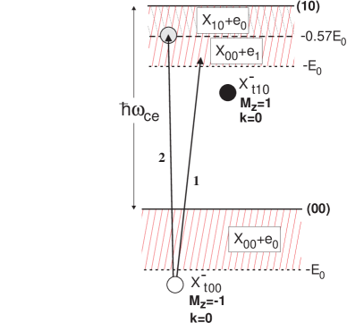
FIG. 1.: Schematic drawing of the $2e$–$h$ electron triplet $S_{e}=1$ eigenstates in zero $(n_{e}n_{h})$=(00) and first electron $(n_{e}n_{h})$=(10) LL’s and the allowed internal transitions from the triplet ground state $X^{-}_{t00}$. The shaded dot indicates the presence within a continuum of a quasi-bound $X^{-}$ state (see the text).

Schematically, the spectra of the triplet $2e$–$h$ eigenstates in two lowest LL’s are shown in Fig. 1. The hatched areas correspond in Fig. 1 to the three-particle continuum. It is formed by the states of the neutral magnetoexciton (MX), which has bound internal $e$–$h$ motion and extended CM motion, [24] and an electron in a scattering state; the latter on average is at infinity from the MX. For the $(n_{e}n_{h})=(10)$ LL’s, there are two different overlapping MX bands. One corresponds to the $X_{00}$ MX ($e$ and $h$ in their zero LL’s) plus a second electron in a scattering state in the first LL. The second, narrow continuum corresponds to the $X_{10}$ MX ($e$ the first and $h$ in the zero LL). The lower continuum edge lies at the $X_{10}$ ground state energy $E_{10}=-0.574E_{0}$, which, for the isolated $X_{10}$, is achieved at a finite CM momentum ${\bf K}_{0}\simeq 1.19\hbar l_{B}^{-1}$. Importantly, this produces in 2D a van Hove singularity in the $X_{10}$ density of states $g_{\rm sing}(E)\simeq M_{01}^{1/2}K_{0}/\pi\hbar\sqrt{E-E_{10}}$, where $M_{10}\simeq 3.62\hbar^{2}/E_{0}l_{B}^{2}$ is the effective [24] $X_{10}$ mass.

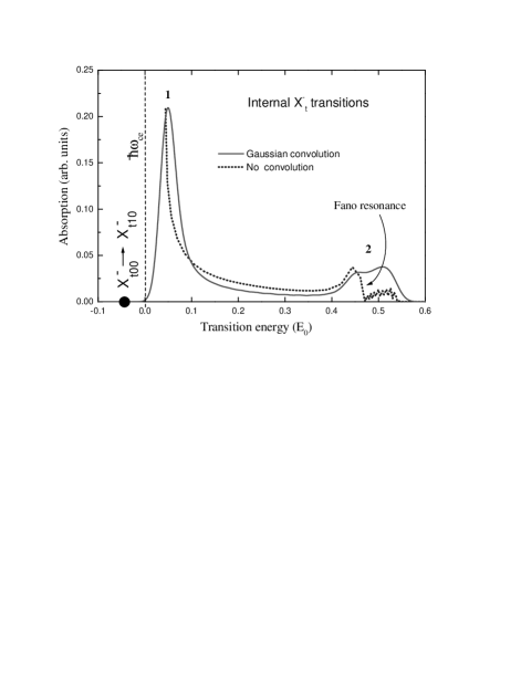
FIG. 2.: Dotted line: spectra of the transitions from the triplet $X^{-}_{t00}$ ground state to the continuum in the first electron LL. Solid line: the spectra convoluted with a Gaussian of the $0.015E_{0}$ width. Labeling of peaks corresponds to Fig. 1. The filled dot shows the position of the forbidden bound-to-bound $X_{t00}^{-}\rightarrow X_{t10}^{-}$ transition.

The bound $X^{-}$ states form discrete spectra and are characterized by bound internal motions of all particles. Such states lie outside the continuum. In the zero LL’s, there is only one bound state — the triplet $X_{t00}$ with a small binding energy $0.044E_{0}$ (counted from the lower continuum edge). [14, 17] In a 2D system in the high-$B$ limit, there are no bound singlet $X^{-}$ states in the zero LL’s. [14] In the next electron LL $(n_{e}n_{h})=(10)$, there is also only one bound state, which is the triplet $X^{-}_{t10}$ with a larger binding energy $0.086E_{0}$.[15, 17] We do not discuss here the discrete excited three-particle states [15] that lie above LL’s.

In addition, quantum mechanical resonances — quasi-bound three particle states — can exist in the continuum. Such a possibility appears plausible for charged 2D MX’s because of the van Hove singularities in the density of states of neutral MX’s. Quasi-bound states, because of long-range oscillating tails, do not have normalizable wave functions. [25] Nevertheless, they have large probabilities of finding all three particles together in real space. In optical transitions quasi-bound states may produce Fano resonances [18] — spectra with highly asymmetric line shapes that are determined by the coupling between a quasi-bound state and a continuum.

We have found spectra of this sort in internal transitions from the 2D triplet $X^{-}_{t00}$ ground state to the next electron LL (Fig. 1). Such $X^{-}$ internal transitions are strong and gain strength with $B$. The transitions must simultaneously satisfy [17] the two exact selection rules: $\Delta k=0$ and $\Delta M_{z}=\pm 1$. Because of the selection rules, the bound-to-bound $X^{-}_{t00}\rightarrow X^{-}_{t10}$ transition turns out to be strictly prohibited in a translationally invariant system. [17] The allowed transitions are therefore photoionizing transitions to the continuum. They have intrinsic linewidths $\sim 0.2E_{0}$ with a sharp onset at the threshold energy that equals $\hbar\omega_{\rm ce}$ plus the $X^{-}_{t00}$ binding energy (transition 1 in Figs. 1, 2). There is also a prominent feature at an energy about $\hbar\omega_{\rm ce}+0.5E_{0}$ — the second peak denoted as transition 2 in Figs. 1, 2. The predicted [17] double-peak structure in the singlet and triplet $X^{-}$ internal photoionizing transitions has been observed [26] in quantum wells in magnetic fields. The positions of the peaks are in good quantitative agreement with calculations performed for realistic parameters of quasi-2D quantum wells at finite fields, as has been described in detail elsewhere. [26, 17] The existence of the second peak has been previously associated [17] with the high density of final states at the lower edge of the $X_{10}+e_{0}$ continuum.

Our present high-accuracy calculations have revealed the fine structure of the second peak. When the spectra are convoluted with the Gaussian of the $0.015E_{0}$ width, which simulates a relatively large inhomogeneous broadening, the second peak has a “camel-back” shape. However, when no artificial broadening is performed, a shape typical [18] for the Fano antiresonance is clearly present in the spectra (Fig. 2). This is an evidence that quasi-bound charged MX’s $X^{-}$ exist within the three-particle continuum. Note that such states are absent in the two-particle spectra of the strictly 2D neutral MX’s that have essentially bound relative $e$–$h$ motion; [24] such states exist for bulk [27] 3D and confined [28] quasi-1D neutral MX’s. We considered here the spectra of internal $X^{-}$ transitions. Resonances that are optically-active in photoluminescence [16] are also expected to exist in the spectra. Experimental search for such resonances require high quality samples with small inhomogeneous broadening.

V Conclusions

We have developed a novel expansion in LL’s that is compatible with both rotations about the ${\bf B}$ axis and magnetic translations. The operator approach allows one to partially separate the center-of-mass from internal degrees of freedom for charged $e$–$h$ systems in magnetic fields. The proposed unitary transformation of the Hamiltonian may be useful in various solid state and atomic physics problems dealing with systems of charged particles in magnetic fields. Here we have considered the 2D systems; however, the developed approach can also be applied to 3D systems [8, 9] for the separation of the coordinates in the plane perpendicular to ${\bf B}$.

We have found evidence that, in addition to discrete bound states, quasi-bound states (resonances) of charged magnetoexcitons $X^{-}$ exist in the continuum of higher Landau levels in 2D systems; this is a qualitatively new feature in the three-particle spectra in a magnetic field. Experimentally, such states may be observed as Fano-resonances in the interband and intraband optical spectra.

The author is grateful to B.D. McCombe for useful discussions. This work was supported in part by COBASE grant and by Russian Ministry of Science program “Nanostructures”.

A Charged $e$–$h$ systems with an arbitrary number of particles

Charged $e$–$h$ complexes, such as charged multiple-excitons [14] $X_{n}^{-}$ and multiply-charged excitons [29] $X^{-k}$, may be bound and stable in quasi-2D systems. Let us demonstrate that for a charged system containing an arbitrary number of $N_{e}$ electrons and $N_{h}$ holes (with, e.g., $N_{e}>N_{h}$), a transformation analogous to (17)–(21) can also be performed. Let us first separate the center-of-masses of the $e$- and $h$- subsystems. This can be done, for example, with the help of the linear orthogonal Jacobi transformation: For the electron coordinates we have $\{{\bf r}_{ei}\}\rightarrow\{\tilde{{\bf r}}_{ei}\}$, where $\tilde{{\bf r}}_{ei}=(\sum_{l=1}^{i}{\bf r}_{el}-i{\bf r}_{ei+1})/\sqrt{i(i+1)}$, $i=1,\ldots,N_{e}-1$ are the internal coordinates and $\tilde{{\bf r}}_{eN_{e}}\equiv{\bf R}_{e}=\sum_{i=1}^{N_{e}}{\bf r}_{ei}/\sqrt{N_{e}}$ is the electron CM coordinate. The analogous transformation is performed for the hole coordinates. Note that the orthogonality of the transformations ensures that the ${\bf R}_{e}$ and ${\bf R}_{h}$ degrees of freedom carry the charges $\mp e$, respectively. [9] We have therefore

$$\hat{k}_{-}=\sqrt{\frac{N_{e}}{N_{e}-N_{h}}}B^{{\dagger}}_{e}({\bf R}_{e})-\sqrt{\frac{N_{h}}{N_{e}-N_{h}}}B_{h}({\bf R}_{h})\,,$$ (A1)

where $B^{{\dagger}}_{e}$ and $B_{h}$ are the $e$- and $h$-CM intra-LL ladder operators. We can now see that, analogously to (17), the Bogoliubov transformation diagonalizing $\hat{\bf k}^{2}$ should involve the intra-LL $e$- and $h$- center-of-mass operators $B^{{\dagger}}_{e}({\bf R}_{e})$ and $B_{h}({\bf R}_{h})$ with $\Theta=\tanh^{-1}(\sqrt{N_{h}/N_{e}})$.

B Electron systems

It is interesting to compare the $e$–$h$ systems with systems of charges of the same sign (e.g., $e_{j}<0$ for all particles $j$). To illustrate this we consider a simplest possible system of two negative charges $e_{1},e_{2}<0$ of masses $m_{1}$ and $m_{2}$. The raising operator $\hat{k}_{-}$ has the form [cf. (16) and (A1)]

$$\hat{k}_{-}=\sqrt{\frac{e_{1}}{e_{1}+e_{2}}}\,B^{{\dagger}}_{e}({\bf r}_{1})+\sqrt{\frac{e_{2}}{e_{1}+e_{2}}}\,B^{{\dagger}}_{e}({\bf r}_{2})\,.$$ (B1)

This can be considered to be a result of the unitary transformation

$${\cal S}B^{{\dagger}}_{e}({\bf r}_{1}){\cal S}^{{\dagger}}=uB^{{\dagger}}_{e}({\bf r}_{1})+vB^{{\dagger}}_{e}({\bf r}_{2})$$ (B2)

where ${\cal S}=\exp(\varphi L)$ with the generator $L=B^{{\dagger}}_{e}({\bf r}_{1})B_{e}({\bf r}_{2})-B^{{\dagger}}_{e}({\bf r}_{2})B_{e}({\bf r}_{1})$. The transformation parameters are given by $u=\cos\varphi=\sqrt{e_{1}/(e_{1}+e_{2})}$ and $v=\sin\varphi=\sqrt{e_{2}/(e_{1}+e_{2})}$. Note that contrary to the $e$–$h$ systems [see Eq. (32)], the vacuum state does not change under this transformation: ${\cal S}|0\rangle=|0\rangle$. Another way of looking at this result is to consider (B2) as a transformation following from the orthogonal transformation of the coordinates

$$\left(\begin{array}[]{c}{\bf R}_{1}\\ {\bf R}_{2}\end{array}\right)=\hat{G}\left(\begin{array}[]{c}{\bf r}_{1}\\ {\bf r}_{2}\end{array}\right)\quad,\quad\hat{G}=\left(\begin{array}[]{rc}\cos\varphi&\sin\varphi\\ -\sin\varphi&\cos\varphi\end{array}\right)\,.$$ (B3)

The matrix $\hat{G}$ is orthogonal, i.e., satisfies $\hat{G}^{\rm T}=\hat{G}^{-1}$. The electron Bose ladder operators are changed according to [cf. with Eqs. (25) and (26)]

$${\cal S}\left(\begin{array}[]{c}B^{{\dagger}}_{e}({\bf r}_{1})\\ B^{{\dagger}}_{e}({\bf r}_{2})\end{array}\right){\cal S}^{{\dagger}}=\hat{G}\left(\begin{array}[]{c}B^{{\dagger}}_{e}({\bf r}_{1})\\ B^{{\dagger}}_{e}({\bf r}_{2})\end{array}\right)=\left(\begin{array}[]{c}B^{{\dagger}}_{e}({\bf R}_{1})\\ B^{{\dagger}}_{e}({\bf R}_{2})\end{array}\right)\,.$$ (B4)

For real parameters of transformation $\varphi$ we deal with O(2) matrices, in general the symmetry group is $SU(2)$. The coordinate representation of the vacuum state $\langle{\bf r}_{1}\ldots{\bf r}_{j}|0\rangle\sim\exp(-\sum_{j}{\bf r}_{j}^{2}/4l_{B}^{2})$ contains a bilinear form in the exponent and is invariant under orthogonal transformations.

The orthonormal basis of states with $k=0$ and $M_{z}=-m$ in, e.g., zero LL is

$$|m\rangle=\frac{1}{\sqrt{m!}}\,[uB^{{\dagger}}_{e}({\bf r}_{1})-vB^{{\dagger}}_{e}({\bf r}_{2})]^{m}|0\rangle\,.$$ (B5)

For $u\neq v$ these states do not have definite parity under the permutation ${\bf r}_{1}\leftrightarrow{\bf r}_{2}$. The Coulomb interaction energies are given by the expectation values $\langle m|U_{\rm ee}({\bf r}_{1}-{\bf r}_{2})|m\rangle$, which solves the problem in the high-field limit. Note that the form of the eigenstates (B5) does not depend on the form of the interaction potential $U_{\rm ee}$ (cf. with Ref. [13]). Note that if the charge-to-mass ratio is the same for all particles, $e_{j}/m_{j}={\rm const}$, the states $(\hat{\pi_{+}})^{n}|m\rangle$ are also exact eigenstates of the Hamiltonian [see Eq. (4)] and correspond to the free CM motion in the $n$-th LL.

C Coulomb matrix elements

In order to perform the infinite summations in (63), it is convenient to obtain first the presentation of the matrix elements (66) using the Fourier transform: Expressing the exponent $\exp(i{\bf q}\!\cdot\!{\bf r})$ in terms of the intra- and inter-LL ladder operators, one obtains [19]

$$U_{n_{1}m_{1}\,pm_{2}}^{n^{\prime}_{1}m^{\prime}_{1}\,pm^{\prime}_{2}}=\int\!\frac{d^{2}q}{(2\pi)^{2}}\,\tilde{U}_{\rm eh}(q)$$ (C1)

$$\times\langle n^{\prime}_{1}|\hat{D}(i\tilde{q}^{\ast})|n_{1}\rangle\,\langle m^{\prime}_{1}|\hat{D}(\tilde{q})|m_{1}\rangle$$ (C2)

$$\times\langle m_{2}|\hat{D}(-\tilde{q})|m^{\prime}_{2}\rangle\,\langle p|\hat{D}(-i\tilde{q}^{\ast})|p\rangle\,.$$ (C3)

Here $\tilde{q}=(q_{x}+iq_{y})l_{B}/\sqrt{2}$ and the matrix elements of the displacement operator [21] $\hat{D}(\alpha)=\exp\left(\alpha A^{{\dagger}}-\alpha^{\ast}A\right)$ between the oscillator eigenstates have, e.g., for $n\leq n^{\prime}$, the form

$$\langle n^{\prime}|\hat{D}(\alpha)|n\rangle=\sqrt{\frac{n!}{n^{\prime}!}}\,\alpha^{n^{\prime}-n}\,e^{-\frac{|\alpha|^{2}}{2}}L_{n}^{n^{\prime}-n}(|\alpha|^{2})\,,$$ (C4)

where $L_{n}^{s}(x)$ are generalized Laguerre polynomials; $L_{n}^{0}(x)=L_{n}(x)$. Using (C4) and the generating function of the Laguerre polynomials [30]

$$\sum_{n=0}^{\infty}L_{n}^{s}(x)z^{n}=\frac{\exp\left(\frac{xz}{z-1}\right)}{(1-z)^{s+1}}\,,\hskip 12.91663pt|z|<1\,,$$ (C5)

we obtain

$$\frac{1}{2}\sum_{p=0}^{\infty}\left(\frac{1}{2}\right)^{p}\langle p|\hat{D}(-i\tilde{q}^{\ast})|p\rangle$$ (C6)

$$=e^{-\frac{x}{2}}\frac{1}{2}\sum_{p=0}^{\infty}\left(\frac{1}{2}\right)^{p}L_{p}(x)=e^{-\frac{3x}{2}}\,,$$ (C7)

where $x=q^{2}l_{B}^{2}/2$. For the matrix elements (63)

$$\bar{U}_{0m_{1}\,0l_{1}}^{0m_{2}\,0l_{2}}\equiv\delta_{l_{1}-m_{1},l_{2}-m_{2}}$$ (C8)

$$\times\bar{U}_{{\rm min}(m_{1},m_{2}),{\rm min}(l_{1},l_{2})}(|m_{1}-m_{2}|)$$ (C9)

we therefore obtain the integral representation

$$\bar{U}_{mn}(s)=\left(\frac{m!n!}{(m+s)!(n+s)!}\right)^{1/2}$$ (C10)

$$\times\int\!\frac{d^{2}q}{(2\pi)^{2}}\,\tilde{U}_{\rm eh}(q)e^{-3x}x^{s+1}\,L_{m}^{s}(x)L_{n}^{s}(x)\,.$$ (C11)

For the Coulomb interactions with the 2D Fourier transform $\tilde{U}_{\rm eh}(q)=-2\pi e^{2}/\epsilon q$, the integral in (C10) can be calculated analytically using the generating function (C5), as has been described in detail elsewhere. [19, 31] The final result is

$$\bar{U}_{mn}(s)=-\frac{E_{0}}{\left[m!(m+s)!n!(n+s)!\right]^{1/2}\,2^{m+n+s}3^{s+1/2}}$$ (C12)

$$\times\sum_{k=0}^{m}\,\sum_{l=0}^{n}\,C_{m}^{k}\,C_{n}^{l}\,\left(\frac{2}{3}\right)^{k+l}\,[2(k+l+s)-1]!!$$ (C13)

$$\times[2(m-k)-1]!!\sum_{p=0}^{n-l}\,C_{k}^{p}\,C_{n-l}^{p}\,(-1)^{p}\,p!\,$$ (C14)

$$\times[2(n-l-p)-1]!!\,.$$ (C15)

REFERENCES

• [1]
• [2] on leave from General Physics Institute, RAS, Moscow 117942, Russia
• [3] W. Kohn, Phys. Rev. 123, 1242 (1961).
• [4] R. S. Knox, Theory of Excitons, Solid State Physics, supplement 5 (Academic Press, New York, 1963).
• [5] J. Zak, Phys. Rev. 134, A1602 (1964); E. Brown, in Solid State Physics, V. 22, Eds. E. Ehrenreich and F. Seitz (Academic Press, New York, 1968).
• [6] L. P. Gor’kov and I. E. Dzyaloshinskii, JETP 26, 449 (1968).
• [7] W. E. Lamb, Phys. Rev. 85, 259 (1952).
• [8] J. E. Avron, I. W. Herbst, and B. Simon, Ann. Phys. (N.Y.) 114, 431 (1978).
• [9] B. R. Johnson, J. O. Hirschfelder, and K. H. Yang, Rev. Mod. Phys. 55, 109 (1983).
• [10] N. R. Cooper and D. B. Chklovskii, Phys. Rev. B 55, 2436 (1997); E. I. Rashba and M. D. Sturge, Phys. Rev. B 63, 045 305 (2000); A. B. Dzyubenko, Phys. Rev. B 64, 241101 (R) (2001) (cond-mat/0106229).
• [11] S. M. Girvin and T. Jach, Phys. Rev. B 29, 5617 (1984).
• [12] Z. F. Ezawa, Quantum Hall Effects (World Scientific, Singapore, 2000).
• [13] V. Pasquier, Phys. Lett. B 490, 258 (2000).
• [14] J. J. Palacios, D. Yoshioka, and A. H. MacDonald, Phys. Rev. B 54, R2296 (1996); A. Wójs, J. J. Quinn, and P. Hawrylak, Phys. Rev. B 62, 4630 (2000); C. Riva, F. M. Peeters, and K. Varga, Phys. Rev. B 63, 115 302 (2001).
• [15] A. B. Dzyubenko, Solid State Commun. 113, 683 (2000).
• [16] See, e.g., K. Kheng, R. T. Cox, Y. Merle d’Aubigne, F. Bassani, K. Saminadayar, and S. Tatarenko, Phys. Rev. Lett. 71, 1752 (1993); A. J. Shields, M. Pepper, M. Y. Simmons, and D. A. Ritchie Phys. Rev. B 52, 7841 (1995); S. Glasberg, G. Finkelstein, H. Shtrikman, and I. Bar-Joseph, Phys. Rev. B 59, R10 425 (1999) and references therein.
• [17] A. B. Dzyubenko and A. Yu. Sivachenko, Phys. Rev. Lett. 84, 4429 (2000).
• [18] U. Fano, Phys. Rev. 124, 1866 (1961).
• [19] A. H. MacDonald and D. S. Ritchie, Phys. Rev. B 33, 8336 (1986).
• [20] D. A. Kirzhnits, Field Theoretical Methods in Many-Body Systems (Pergamon Press, Oxford, 1967), p. 372.
• [21] J. R. Clauder and B.-S. Skagerstam, Coherent States. Application in Physics and Mathematical Physics (World Scientific, Singapore, 1985); W.-M. Zhang, D. H. Feng, and R. Gilmore, Rev. Mod. Phys. 62, 867 (1990).
• [22] For work on single-particle coherent and squeezed states in magnetic fields see I. A. Malkin and V. I. Man’ko, JETP 28, 527 (1969); A. Feldman and A. H. Kahn, Phys. Rev. B 1, 4584 (1970); E. I. Rashba, L. E. Zhukov, and A. L. Efros, Phys. Rev. B 55, 5306 (1997); M. Ozana and A. L. Shelankov, Fiz. Tverd. Tela 40, 1405 (1998) [Phys. Solid State 40, 1276 (1998)] and references therein.
• [23] For a system of charges of the same sign (e.g., $e_{j}<0$) a diagonalization of the operator $\hat{k}_{-}$ does not produce a coherent state as a new vacuum state (see Appendix B).
• [24] I. V. Lerner and Yu. E. Lozovik, JETP 51, 588 (1980).
• [25] A. I. Baz’, Ya. B. Zel’dovich, and A. M. Perelomov, Scattering, Reactions and Decay in Non-Relativistic Quantum Mechanics (Israel Program for Scientific Translations, Jerusalem, 1969).
• [26] H. A. Nickel, G. S. Herold, T. Yeo, G. Kioseoglou, Z. X. Zhiang, B. D. McCombe, A. Petrou, D. Broido, and W. Schaff, Phys. Stat. Sol. B 210, 341 (1998); A. B. Dzyubenko, A. Yu. Sivachenko, H. A. Nickel, T. M. Yeo, G. Kioseoglou, B. D. McCombe, and A. Petrou, Physica E 6, 156 (2000).
• [27] S. Glutsch, U. Siegner, M.-A. Mycek, and D. S. Chemla, Phys. Rev. B 50, 17 009 (1994); U. Siegner, M.-A. Mycek, S. Glutsch, and D. S. Chemla, Phys. Rev. B 51, 4953 (1995).
• [28] M. Graf, P. Vogl, and A. B. Dzyubenko, Phys. Rev. B 54, 17 003 (1996).
• [29] V. I. Yudson, Phys. Rev. Lett. 77, 1564 (1996).
• [30] I. S. Gradshtein, I. M. Ryzhik, Table of Integrals, Series, and Products (Academic, San Diego, 1980).
• [31] A. B. Dzyubenko, Sov. Phys. Solid State 34, 1732 (1992).