DOES BERRY PHASE EXIST FOR A SYSTEM COUPLED TO ITS ENVIRONMENT?

Berry phase was originally defined for systems whose states are separated by finite energy gaps. One might naively expect that a system without a gap cannot have a Berry phase. Despite this we ask whether a Berry phase can be observed in a system which has a continuous spectrum because its coupling to the environment has broadened its energy levels. We find that, contrary to the above naive expectation, there are conditions under which the Berry phase is observable. However it is modified by the presence of the environment and no longer has a simple geometric interpretation. The model system we consider is a spin-half in a slowly rotating magnetic field, with the spin also coupled to a Ohmic environment of harmonic oscillators (spin-boson model). Here we discuss the high-temperature limit of this model. We then interpret our results in terms of a spin under the influence of a classical stochastic field.

1 Motivation and Summary

Originally Berry phase $\!{}^{{\bf?}}$ was defined for systems whose states were separated by finite energy gaps. Here we ask whether a Berry phase can be observed in a system whose spectrum is continuous, more specifically: a system which is not completely isolated from its environment. All real systems are coupled, at least weakly, to their environment and as a result never have a truly discrete energy level spectrum. The naive argument would be that, since the spectrum of the system does not have a gap, the parameters in the Hamiltonian could never be varied slowly enough to be considered adiabatic. This in turn would mean one could not observe a Berry phase in such a system. If this were the case one could never observe a Berry phase.

The above argument must be too naive: experiments have been carried out which do observe the Berry phase, both directly and indirectly $\!{}^{{\bf?},{\bf?},{\bf?}}$. We therefore take a simple model in which a quantum system which exhibits a Berry phase is coupled to many other quantum degrees of freedom. We then ask two questions. Firstly, under what conditions can the Berry phase be observed? Secondly, is the observed Berry phase the same as that of the isolated system, and if not is it still geometric in nature? While others have investigated systems with Berry phases coupled to other degrees of freedom $\!{}^{{\bf?},{\bf?},{\bf?}}$, we believe we are the first to explicitly ask these two questions.

We should make it clear that we distinguish between the system and the environment in the following way. The system is something which we have experimental control over. Thus we can prepare the system in any state we like and choose all parameters in the Hamiltonian under which it evolves. The environment consists of all the degrees of freedom over which we have little experimental control. Usually the most we can do to the environment is to ensure the universe (system $+$ environment) is in thermal equilibrium, with a temperature $T$. If we are able to take $T$ to zero, then we can prepare the universe in its ground state. However to measure a Berry phase, we must devise a procedure for measuring the phase evolution of this state and getting rid of the dynamic part of the phase. Most such procedures involve the mixing of a large number of eigenstates (of the universe), and hence will lead to dephasing as is discussed below $\!{}^{{\bf?}}$. This implies that the extremely interesting recent work of Avron and Elgart $\!{}^{{\bf?}}$ — on adiabatic evolution of eigenstates of models similar to ours — is not directly relevant to our work.

We choose to investigate a spin-half which is coupled to both a magnetic field and an environment. When isolated from its environment, this spin exhibits a Berry phase if we slowly rotate the magnetic field around a closed loop. We model the environment as a bath of harmonic oscillators coupled to the spin. This model has been chosen for its simplicity, despite this it is relevant to recent suggestions for using Berry phases to control the qubits in a quantum computer $\!{}^{{\bf?},{\bf?}}$. This is of interest because the coupling to the environment is significant for most physical realisations of qubits. While we make no attempt to accurately model the real coupling between the qubit and its environment, we believe our results give an indication of what to expect in the real system.

In this article we concentrate on the case where the frequencies of the oscillators have been chosen so that the bath is Ohmic $\!{}^{{\bf?}}$, and these oscillators are initially at a high-temperature. We find that coupling the spin-half to this type of environment causes four effects. (i) Exponential decay to a state in which the spin is thermalised with the bath, the time-scale associated with this is the spin flip time, $T_{1}$. (ii) Exponential decay of observables containing phase information, the time-scale associated with this is the dephasing time, $T_{2}$. (iii) A Lamb shift $\!{}^{{\bf?}}$ of the energy-levels of the spin by an amount, $\delta E$. (iv) A modification to the Berry phase, $\delta\Phi_{\rm Berry}$. All four of these effects go like the second power of the coupling between the spin and its environment, the functional form of the results are given in Eq. (4). Of these (ii) and (iv) are of most interest to us. Effect (ii) tells us when we can measure the Berry (or any other) phase, while effect (iv) tells us what the Berry phase we measure will be.

Effect (ii) means that one cannot perform an arbitrarily long experiment to measure a phase. Even the most sensitive experiment will not be able to measure the phase if the time of the experiment is much larger than $T_{2}$, because of the exponential decay of the observables containing the phase information. This constraint on the time of the experiment is particularly relevant for Berry phase experiments, since they must be carried out over long times to ensure adiabaticity. So what is the Berry phase for an experiment in which the parameters of the Hamiltonian are taken around a closed loop in a finite time, $t_{\rm period}$? The Berry phase is the component of the phase which is independent of $t_{\rm period}$. Other contributions to the total phase are the dynamic phase which scales linearly with with $t_{\rm period}$, and non-adiabatic contributions which are proportional to $t_{\rm period}$ to some negative power. Clever experiments (see Section 3) can remove the dynamic phase but not the non-adiabatic contributions. One can argue that the Berry phase is present even for very fast experiments, it is just that then it is masked by the non-adiabatic contributions to the phase. For the Berry phase to be accurately measured it must be much larger than the non-adiabatic contributions to the total phase. This can only be achieved by carrying out the experiment slowly enough.

Let us assume that during an experiment on a spin-half in a magnetic field, $\mbox{\boldmath${B}$}(t)$, we slowly change the direction of the field while keeping its magnitude fixed. Then at all times the energy gap between the up and down state is $g\mu B$, where $B=\left|{\mbox{\boldmath${B}$}(t)}\right|$ is time-independent, $g$ is the Landé g-factor, and $\mu\equiv{e\hbar\over 2mc}$ is the Bohr magneton. In this case the non-adiabatic contribution to the phase accumulated over a time, $t$, is of order $\hbar/(g\mu Bt)$. To measure the Berry phase — which is of order one — the non-adiabatic contributions to the total phase must be much less than one. Thus the time of the experiment should satisfy $t_{\rm period}\gg\hbar/(g\mu B)$. If dephasing occurs on a time-scale $T_{2}$ then we cannot measure the total phase for times larger than $T_{2}$. Unless $g\mu BT_{2}/\hbar\gg 1$ the non-adiabatic contributions to the total phase in an experiment which takes time $T_{2}$ will not be small enough for us to accurately measure the Berry phase.

Now that we understand the conditions under which we can measure the Berry phase, we ask if the Berry phase is purely geometric. The answer is no. Effect (iv) tells us that in general there are environment-induced contributions to the Berry phase which are not geometric in nature. Remember we are choosing to define the Berry phase as any contribution to the total phase which is independent of the time, $t_{\rm period}$, that it takes to vary the parameters of the system Hamiltonian around a closed loop. Is this non-geometric contribution to the Berry phase observable? It can be very large, but only if the coupling to the environment is large, in which case the experiment dephases quickly. Then a Berry phase measurement carried out before the system dephases will have significant non-adiabatic contributions to the total phase which may mask $\delta\Phi_{\rm Berry}$. Therefore the environment-induced contribution to the Berry phase can only be observed if

$$\delta\Phi_{\rm Berry}\mbox{\raisebox{2.7pt}{$>$}\hskip-9.0pt\raisebox{-2.6pt}{$\sim$}}{\hbar\over g\mu BT_{2}}.$$ (1)

Only then is $\delta\Phi_{\rm Berry}$ of the same order or larger than the non-adiabatic corrections to the phase that occur when the experiment is carried out in a time $t_{\rm period}\sim T_{2}$. If we look at the functional form of $T_{2}$ and $\delta\Phi_{\rm Berry}$ in (4) we see that there are a wide range of parameters for which $\delta\Phi_{\rm Berry}\sim{\hbar\over g\mu BT_{2}}$. In this parameter range the environment-inducted correction to the Berry phase is just about observable in an experiment which takes a time $t_{\rm period}\sim T_{2}$.

The remainder of this article is arranged as follows. In Section 2 we discuss the model and summarise our results for a high-temperature Ohmic bath. Then in Section 4 we describe the high-temperature Ohmic environment as a randomly-fluctuating magnetic field, and thus develop a more intuitive understanding of one limit of this model. To do this we first give a brief summary of Berry phase for an isolated spin (Section 3).

2 The model and high-temperature results

We will discuss the details of the derivation of the results elsewhere $\!{}^{{\bf?}}$; here we give a very brief overview of the derivation. We start with the following Hamiltonian,

$${\cal H}=-{g\mu\over 2}\mbox{\boldmath${B}$}(t)\cdot\hat{\mbox{\boldmath${\sigma}$}}-{g\mu\over 2}\sum_{i}C\hat{q}_{i}\hat{\sigma}_{z}+\sum_{i}\left[{{\hat{p}_{i}^{2}\over 2m}+{m\Omega_{i}^{2}\hat{q}_{i}^{2}\over 2}}\right].$$ (2)

It is a spin-boson model $\!{}^{{\bf?}}$ with a time-dependent field, ${B}$(t). We consider an Ohmic bath of oscillators with an upper frequency cut-off, $\Omega_{\rm max}$, thus

$$\sum_{i}\left({\cdots}\right)_{\Omega_{i}}=\alpha\int_{0}^{\infty}{\rm d}\Omega\ \Omega^{2}{\rm e}^{-\Omega/\Omega_{\rm max}}\left({\cdots}\right)_{\Omega}$$ (3)

We write the spin operators as operators on a two fermionic system $\sigma_{z}=f^{\dagger}_{1}f_{1}-f^{\dagger}_{2}f_{2}$, $\sigma_{+}=f^{\dagger}_{1}f_{2}$ and $\sigma_{-}=f^{\dagger}_{2}f_{1}$, we then write the Feynman propagator for the system as a coherent-states path integral in which the fermionic degrees of freedom represented by Grassman variables. We integrate out the oscillators exactly $\!{}^{{\bf?},{\bf?}}$. The effective action of the resulting path integral contains a term which is quartic in the fermionic degrees of freedom and couples the state of the spin at time $t_{1}$ to the state of the spin at time $t_{2}$. We carry out a perturbation expansion of this quartic term. We then use the fact that for an Ohmic bath the coupling between the spin state at $t_{1}$ and $t_{2}$ is dominated by $t_{1}-t_{2}\sim\Omega_{\rm max}^{-1}$. Thus in the limit where the time of the experiment $t\gg\Omega_{\rm max}^{-1}$, the perturbation expansion is dominated by a certain class of diagrams that we can sum to all orders.

Here we only discuss results for a high-temperature Ohmic environment. By high-temperature we mean that $k_{\rm B}T\gg\hbar\Omega_{\rm max}$, other limits are discussed in reference 8. For concreteness we take the case where the field $\mbox{\boldmath${B}$}(t)=B\left({\hat{\mbox{\boldmath${x}$}}\sin\theta\cos\omega t+\hat{\mbox{\boldmath${y}$}}\sin\theta\sin\omega t+\hat{\mbox{\boldmath${z}$}}\cos\theta}\right)$ in an experiment which takes a time $t_{\rm period}=2\pi/\omega$. The results — written in terms of the dimensionless coupling between the spin and the oscillators $\tilde{C}=g\mu C\left({\alpha/m\hbar}\right)^{1/2}$ — are as follows,

$${1\over T_{1}} = {\pi\tilde{C}^{2}(k_{\rm B}T)\over 2\hbar}{\rm e}^{-\gamma}\sin^{2}\theta\qquad\qquad\qquad\qquad{1\over T_{2}}\ =\ {\pi\tilde{C}^{2}(k_{\rm B}T)\over 4\hbar}\left({2\cos^{2}\theta+{\rm e}^{-\gamma}\sin^{2}\theta}\right)$$

$${\delta E\over\hbar} = {\tilde{C}^{2}(k_{\rm B}T)\over 4\hbar}f(\gamma)\sin^{2}\theta\qquad\qquad\quad\quad\ \delta\Phi_{\rm Berry}\ =\ {\pi\tilde{C}^{2}(k_{\rm B}T)\over 2\hbar\Omega_{\rm max}}f^{\prime}(\gamma)\sin^{2}\theta\cos\theta$$ (4)

where $\gamma=g\mu B/\hbar\Omega_{\rm max}$. The function $f(x)={\rm e}^{x}{\rm Ei}(-x)-{\rm e}^{-x}{\rm Ei}(x)$ where we define ${\rm Ei}(x)$ as the principal-value of the Exponential integral, $\int_{-x}^{\infty}{\rm d}t{\rm e}^{-t}/t$. Hence $f^{\prime}(x)\equiv{{\rm d}\over{\rm d}x}f(x)={\rm e}^{x}{\rm Ei}(x)+{\rm e}^{-x}{\rm Ei}(-x)$.

3 Berry phase for an isolated spin : Rotating reference frame trick

Consider a spin-half coupled to a magnetic field, $\mbox{\boldmath${B}$}(t)$, via the Hamiltonian,

$${\cal H}=-{g\mu\over 2}\mbox{\boldmath${B}$}(t)\cdot\hat{\mbox{\boldmath${\sigma}$}}$$ (5)

Now imagine that the magnetic field rotates with angular velocity, $\mbox{\boldmath${\omega}$}(t)$, so that ${{\rm d}\over{\rm d}t}\mbox{\boldmath${B}$}(t)=\mbox{\boldmath${\omega}$}(t)\times\mbox{\boldmath${B}$}(t)$. We can go to a reference frame which rotates with the ${B}$-field. In this new non-inertial frame the spin experiences a pseudo-field, as well as the time-independent field $\mbox{\boldmath${B}$}^{\prime}=\mbox{\boldmath${B}$}(0)$. The pseudo-field is simply $-\hbar\mbox{\boldmath${\omega}$}(t)/g\mu$. Thus all the time-dependence in the problem has been moved from ${B}$ to ${\omega}$. In the rotating frame the Hamiltonian is

$${\cal H}^{\prime}=-{g\mu\over 2}\left[{\mbox{\boldmath${B}$}^{\prime}-{\hbar\over g\mu}\mbox{\boldmath${\omega}$}(t)}\right]\cdot\hat{\mbox{\boldmath${\sigma}$}}.$$ (6)

Note that if we transform the initial state to the rotating frame, evolve it using ${\cal H}^{\prime}$, then transform back to the non-rotating frame, we end up with a final state $\big{|}\psi_{f}^{\prime}\big{>}$. Careful analysis shows that the true final state is actually $\big{|}\psi_{f}\big{>}={\rm e}^{{\rm i}\phi\hat{\sigma}_{z}}\big{|}\psi_{f}^{\prime}\big{>}$, however in all cases we will consider $\phi$ is a multiple of $\pi$. The resulting sign difference between $\big{|}\psi_{f}\big{>}$ and $\big{|}\psi_{f}^{\prime}\big{>}$ will be of no consequence and can be ignored.

The power of transforming to the rotating frame becomes clear if we consider a rotation of the ${B}$-field for which ${\omega}$ is time-independent. Then the transformation turns a time-dependent problem into a time-independent one. The time-independent problem can then be solved by working in the basis where ${\cal H}^{\prime}$ is diagonal.

We consider the following experiment to measure the Berry phase. We start with a ${B}$-field, $\mbox{\boldmath${B}$}(0)=B\left({\hat{\mbox{\boldmath${x}$}}\sin\theta+\hat{\mbox{\boldmath${z}$}}\cos\theta}\right)$, which we then rotate with angular velocity $\mbox{\boldmath${\omega}$}=\hat{\mbox{\boldmath${z}$}}\omega$ for a time $t_{\rm period}=2\pi/\omega$. In the limit $\omega\to 0$, the component of the spin-state which is initially up relative to $\mbox{\boldmath${B}$}(0)$ acquires a phase $\Phi={\textstyle{\frac{1}{2}}}\Theta+\int_{0}^{t_{\rm period}}E_{\uparrow}(t){\rm d}t$, while the state which is initially down acquires a phase equal to $-\Phi$. The first term in $\Phi$ is the Berry phase (for a spin-half), $\Phi_{\rm Berry}={\textstyle{\frac{1}{2}}}\Theta$, where $\Theta=2\pi\left({1-\cos\theta}\right)$ is the solid-angle enclosed by the path the ${B}$-field takes in the non-rotating frame. The second term is the dynamic phase, $\Phi_{\rm dyn}=\int_{0}^{t_{\rm period}}E_{\uparrow}(t){\rm d}t$, where $E_{\uparrow}(t)={\textstyle{\frac{1}{2}}}g\mu B$ is the energy of the instantaneous eigenstate at time $t$.

We are in the adiabatic limit, which means that the dynamic phase is much larger than the Berry phase. If we wish to carry out an experiment which yields the Berry phase, rather than the sum of the Berry and dynamic phases, then we can eliminate the dynamic phase using the following spin-echo technique $\!{}^{{\bf?}}$. We (a) adiabatically rotate the ${B}$-field around a closed loop, then (b) flip the spin, (c) rotate the field in the opposite direction round the same closed loop, and (d) flip the spin again. By flip the spin, we mean $\left|{\uparrow}\right>\leftrightarrow\left|{\downarrow}\right>$ where the up and down states are defined relative to the direction of ${B}$-field at that time. This can be achieved by applying a fast $\pi$-pulse in a direction perpendicular to the ${B}$-field. When we do (a)-(d) the Berry phases of the first and second loop add up, while the dynamic phases cancel. Thus the phase acquired by the spin is purely dependent on the Berry phase round the loop.

Thus we will consider a field, $\mbox{\boldmath${B}$}(t)$, which rotates with angular velocity $\mbox{\boldmath${\omega}$}=\hat{\mbox{\boldmath${z}$}}\omega$ for $0<t<t_{\rm period}$ (where $t_{\rm period}=2\pi/\omega$) and $\mbox{\boldmath${\omega}$}=-\hat{\mbox{\boldmath${z}$}}\omega$ for $t_{\rm period}<t<2t_{\rm period}$, with a spin flip at time $t_{\rm period}$ and time $2t_{\rm period}$. Then the probability of an initial state $\left|{u_{0},v_{0}}\right>=u_{0}\left|{\uparrow}\right>+v_{0}\left|{\downarrow}\right>$ ending up in a state $\left|{u,v}\right>$ at time $2t_{\rm period}$ is

$$P\left({\left|{u,v}\right>,2t_{\rm period};\left|{u_{0},v_{0}}\right>}\right) = \left|{\left<{u,v}\right|\hat{\sigma_{x}}\exp\left[{{\rm i}\Phi(-\omega)\hat{\sigma}_{z}}\right]\hat{\sigma_{x}}\exp\left[{{\rm i}\Phi(\omega)\hat{\sigma}_{z}}\right]\left|{u_{0},v_{0}}\right>}\right|^{2}$$ (7)

$$= u^{*}uu_{0}^{*}u_{0}+v^{*}uv_{0}^{*}u_{0}{\rm e}^{{\rm i}4\Phi_{\rm Berry}}+u^{*}vu_{0}^{*}v_{0}{\rm e}^{-{\rm i}4\Phi_{\rm Berry}}+v^{*}vv_{0}^{*}v_{0}$$

where all spin-states are defined relative to the axis of the field $\mbox{\boldmath${B}$}(0)$.

4 Berry phase and decoherence in a randomly fluctuating magnetic field

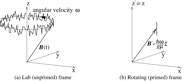
Figure 1: Here we show the magnetic field discussed in Section 4, in both the laboratory frame (a) and the rotating frame (b). The smooth line in (a) is the time-dependence of the field, $\mbox{\boldmath${B}$}(t)$, while the irregular line represent the total field, $\left({\mbox{\boldmath${B}$}(t)+\hat{\mbox{\boldmath${z}$}}K(t)}\right)$. It fluctuates wildly because $K(t)$ fluctuates randomly with time. In the rotating frame (b) both the field $\mbox{\boldmath${B}$}^{\prime}$ and the pseudo-field $\left({-\hat{\mbox{\boldmath${z}$}}\hbar\omega/g\mu}\right)$ are time-independent, while the field $K(t)$ fluctates. The vertical double-ended arrow represent the fluctuations of the total field, $\left({\mbox{\boldmath${B}$}^{\prime}-\hat{\mbox{\boldmath${z}$}}\hbar\omega/g\mu+\hat{\mbox{\boldmath${z}$}}K(t)}\right)$.

A spin in an experimentally controlled magnetic field $\mbox{\boldmath${B}$}(t)$ with a $z$-axis coupling to a high-temperature Ohmic bath of oscillators is equivalent to the spin in a field $\mbox{\boldmath${B}$}(t)+\mbox{\boldmath${K}$}(t)$ where $\mbox{\boldmath${K}$}(t)=\hat{\mbox{\boldmath${z}$}}K(t)$ is a randomly-fluctuating field $\!{}^{{\bf?}}$. The Hamiltonian for this model is simply ${\cal H}=-{g\mu\over 2}\left[{\mbox{\boldmath${B}$}(t)+\hat{\mbox{\boldmath${z}$}}K(t)}\right]\cdot\hat{\mbox{\boldmath${\sigma}$}}$. If there is an upper cut-off on the frequencies of the oscillator, $\Omega_{\rm max}$, then $K(t)$ is Gaussianly distributed and uncorrelated for times longer than $\Omega_{\rm max}^{-1}$. Thus on time-scales much greater than $\Omega_{\rm max}^{-1}$ we can average over $K(t)$ using,

$$\left<{\cdots}\right>={\int\left[{{\textstyle\prod_{j=0}^{N-1}}{\rm d}K_{j}}\right](\cdots)\exp\left[{-{\epsilon\over 2\kappa^{2}}\sum_{j=0}^{N-1}K_{j}^{2}}\right]\over\int\left[{{\textstyle\prod_{j=0}^{N-1}}{\rm d}K_{j}}\right]\exp\left[{-{\epsilon\over 2\kappa^{2}}\sum_{j=0}^{N-1}K_{j}^{2}}\right]}$$ (8)

where $K_{j}\equiv K(j\epsilon)$ and the period of each time-slice $\epsilon=t/N$. We require that $\epsilon$ is of the order or larger than $\Omega_{\rm max}^{-1}$. This random-field model is equivalent to the Ohmic high-temperature bath of oscillators with

$$\kappa^{2}={\alpha\pi C^{2}(k_{\rm B}T)\over m}={\pi\hbar\tilde{C}^{2}(k_{\rm B}T)\over g^{2}\mu^{2}}.$$ (9)

In general this equivalence does not aid our calculations. However there is one limit for which the random-field interpretation enables us to derive the results in a much simpler and more intuitive manner. This is the limit in which $\Omega_{\rm max}\ll g\mu B/\hbar$. Then the spin in the random field model can adiabatically follow the field $\mbox{\boldmath${B}$}(t)+\hat{\mbox{\boldmath${z}$}}K(t)$, because $K(t)$ varies smoothly on time-scales of order $\Omega_{\rm max}^{-1}\gg\hbar/(g\mu B)$. The exact requirement for the spin to adiabatically follow the field is that at all times

$${{\rm d}\over{\rm d}t}\left[{\mbox{\boldmath${B}$}(t)+\hat{\mbox{\boldmath${z}$}}K(t)\over\left|{\mbox{\boldmath${B}$}(t)+\hat{\mbox{\boldmath${z}$}}K(t)}\right|}\right]\ll{g\mu\over\hbar}\left|{\mbox{\boldmath${B}$}(t)+\hat{\mbox{\boldmath${z}$}}K(t)}\right|.$$ (10)

We assume that fluctuations in $K$ are given by $\big{<}K^{2}\big{>}^{1/2}\sim\kappa\Omega_{\rm max}^{1/2}$ for time-scales greater than $\Omega_{\rm max}^{-1}$, while $K$ varies smoothly on time-scales shorter than that. If $B\gg\big{<}K^{2}\big{>}^{1/2}$ then we do not need any detailed information on the dynamics of $K$ on these short time-scales. We will restrict ourselves to the limit where $B\gg\big{<}K^{2}\big{>}^{1/2}$ and $B\gg\hbar\Omega_{\rm max}/g\mu$. Hence the adiabaticity condition, Eq. (10), is reduced to $\kappa\Omega_{\rm max}^{3/2}/B^{2}\ll 1$, which is automatically fulfilled in this limit. The limit defined by these approximations is easy to work in because it is only in this limit that we are allowed to take the adiabatic limit first and then do the averaging.

If we consider the same time-dependence for $\mbox{\boldmath${B}$}(t)$ as we did for the isolated spin, then we can simplify the problem significantly by going to the reference frame which rotates with $\mbox{\boldmath${B}$}(t)$, see Fig. 1. Remember that in the non-rotating frame $K(t)$ fluctuates in the $\hat{\mbox{\boldmath${z}$}}$-direction. Thus it unaffected by going to the rotating frame, in other words $\mbox{\boldmath${K}$}^{\prime}(t)$ as $\mbox{\boldmath${K}$}(t)$. In the frame which rotates with angular velocity $\mbox{\boldmath${\omega}$}=\pm\hat{\mbox{\boldmath${z}$}}\omega$ the total phase acquired in time, $t_{\rm period}$, is simply the dynamic phase in this rotating frame,

$$\Phi(\pm\omega)={g\mu\over 2\hbar}\int_{0}^{t_{\rm period}}\left|{\mbox{\boldmath${B}$}^{\prime}\mp(\hbar/g\mu)\hat{\mbox{\boldmath${z}$}}\omega+\hat{\mbox{\boldmath${z}$}}K(t)}\right|{\rm d}t$$ (11)

The path of $\left({\mbox{\boldmath${B}$}(0)\mp(\hbar/g\mu)\hat{\mbox{\boldmath${z}$}}\omega+\hat{\mbox{\boldmath${z}$}}K(t)}\right)$ encloses no area in the rotating frame, so there is no Berry phase in this frame. It is important to remember that this does not mean there is no Berry phase in the laboratory frame. We have already seen this for the case where $\hat{\mbox{\boldmath${z}$}}K(t)=0$. Then there is no Berry phase in the rotating frame, but there is in the laboratory frame (as shown in Section 3). To identify the Berry phase we must first ensure $\omega=2\pi/t_{\rm period}$, the Berry phase will then be the $t_{\rm period}$-independent component of the total phase.

We now wish to calculate the averaged propagation probability for evolution under the time-dependent ${B}$-field described in Section 3. Before averaging the propagation probability is given by (7) with the phase $4\Phi_{\rm Berry}$ replaced by $2\left[{\Phi(\omega)-\Phi(-\omega)}\right]$, where $\Phi(\pm\omega)$ are given in (11). We can then average using (8). While in general carrying out the averaging is difficult, it is straightforward in the limit we are considering — $B\gg\big{<}K^{2}\big{>}^{1/2}$ and $B\gg\hbar\Omega_{\rm max}/g\mu$. We will time-slice the propagator, writing the integral over time in the exponent as a sum of $N$ time-slices each of which takes a time $\epsilon=t/N$. We use (8) to average the propagation probability, by evaluating a few Gaussian integrals. We find the random fluctuations of $K(t)$ cause the phase to acquire an imaginary part and an extra real part. The former causes an exponential decay of all in terms containing phase information. The latter means that the phase which is observed is different from the $K(t)=0$ case. We extract the contributions to the Berry phase by finding the parts of the total phase which which are independent of $t_{\rm period}$. Similarly the contribution to the dynamic phase is the part of the total phase which scales linearly with $t_{\rm period}$. We then interpret the $\kappa$-dependent contribution to the dynamic phase as being a Lamb shift of the energy levels. In the language introduced in Section 1,

$${1\over T_{1}} = 0\qquad\qquad\qquad\qquad\qquad\qquad\qquad\quad\hskip 1.4457pt\ \ {1\over T_{2}}\ =\ {1\over 2}\left({g\mu\kappa\over\hbar}\right)^{2}\cos^{2}\theta$$

$${\delta E\over\hbar} = {1\over\#}{g\mu\kappa^{2}\Omega_{\rm max}\over 2\hbar B}\sin^{2}\theta\qquad\qquad\quad\quad\ \delta\Phi_{\rm Berry}\ =\ {1\over\#}{\pi\kappa^{2}\Omega_{\rm max}\over 2B^{2}}\sin^{2}\theta\cos\theta.$$ (12)

where $\#=\epsilon\Omega_{\rm max}$ is a integer larger than one but still of order one. This means that the results are not independent of our choice of time-slicing for the averaging. This is not surprising since there is a time-scale ($\Omega_{\rm max}$) below which the field $K(t)$ is highly-correlated. This calculation is not sophisticated enough to tell us what $\#$ should be. However we can compare (12) with (4) using (9) and the large-$x$ expansion of the Exponential integral, ${\rm Ei}(x)=-{\rm e}^{x}\left({x^{-1}+x^{-2}+\cdots}\right)$. In this case we see the two sets of results agree completely if we set $\#=\pi$.

This derivation makes it very clear that $T_{1}\to\infty$ in this limit because slow fluctuations of the field can dephase but not flip the spin. It also shows — in a more transparent manner than the calculation discussed in Section 2 — that the environment can modify the dynamic and Berry phases.

References

References

- [1] M.V. Berry, Proc. R. Soc. Lond. 392, 45 (1984).
- [2] See references in the following review letter J. Anandan, J. Christian and K. Wanelik,Am. J. Phys. 65, 180 (1997).
- [3] See for example D.J. Thouless, Topological quantum numbers in non-relativistic physics (World Scientific, Singapore, 1998).
- [4] P. Ao and D.J. Thouless, Phys. Rev. Lett. 70, 2158 (1993). X.-M. Zhu, E. Brändström, and B. Sundqvist, Phys. Rev. Lett. 78, 122 (1997).
- [5] F. Gaitan, Phys. Rev. A 58, 1665 (1998).
- [6] P. Ao and X.-M. Zhu, Phys. Rev. B 60, 6850 (1999).
- [7] J.E. Avron and A. Elgart, Phys. Rev. A 58, 4300 (1998); Comm. Mat. Phys. 203, 445 (1999).
- [8] R.S. Whitney and Y. Gefen – to be published.
- [9] J.A. Jones, V. Vedral, A. Ekert and G. Castagnoli, Nature 403, 869 (2000). A. Ekert, M. Ericsson, P. Hayden, H. Inamori, J.A. Jones, D.K.L.Oi and V. Vedral , J. Mod. Opt. 47, 2501 (2000).
- [10] G. Falci, R. Fazio, G.M. Palma, J. Siewert and V. Vedral, Nature 407, 355 (2000).
- [11] A.O. Caldiera and A.J. Leggett, Physica 121A, 587 (1983); Ann. Phys. 149, 374 (1983).
- [12] See for example S.S. Schweber, An Introduction to Relativistic Quantum Field Theory (Row Peterson, Evanston, 1961).
- [13] A.J. Leggett, S. Chakravarty, A.T. Dorsey, M.P.A. Fisher, A. Garg and W. Zwerger, Rev. Mod. Phys. 59, 1 (1987), and references therein.
- [14] R.P. Feynman and F.L. Vernon, Ann. Phys. 24, 118 (1963).