Multifractal wavelet filter of natural images

Abstract

Natural images are characterized by the multiscaling properties of their contrast gradient, in addition to their power spectrum. In this work we show that those properties uniquely define an intrinsic wavelet and present a suitable technique to obtain it from an ensemble of images. Once this wavelet is known, images can be represented as expansions in the associated wavelet basis. The resulting code has the remarkable properties that it separates independent features at different resolution level, reducing the redundancy, and remains essentially unchanged under changes in the power spectrum. The possible generalization of this representation to other systems is discussed.

Pacs: 87.57.Nk,47.53.+n,87.19.Dd,42.66.Lc

Physical Review Letters, 85, 3325-3328 (2000)

I Introduction

Given the complexity and degree of redundancy of natural images, the early visual system had to find good coding procedures to represent the visual stimuli internally. To achieve this goal, the visual system must have learnt the regularities present in the environment where the organism lived [1]. If there are image features that tend to appear together, a cell responding quasi-optimally to them is rather likely to exist. To find such a representation one has first to understand the statistical properties of visual scenes common in the environment. In particular, the relevance of the second order statistics has been pointed out some time ago [2], and internal representations that eliminate these correlations have been discussed [3]. However, even if whitening represents an improvement of the code, it still leaves much geometrical structure that should be dealt with more properly [4]. A more systematic study of statistical regularities that go beyond the two-point correlations has began rather recently [5, 6, 7]. A novel approach to understand the statistical properties of natural images has been proposed in [6] where the non-gaussian statistics of changes in contrast has been characterized and explained by means of a stochastic multiplicative process: Contrast changes at a given scale are obtained from those at a coarser scale by multiplication with an independent random variable. This implies a linear relation between the logarithms of the variables at two different scales (this property has also been discussed in [9], although the existence of a multiplicative process was not noticed). A very rich geometrical structure has emerged from those studies: contrast changes are organized in such a way that pixels in the image can be classified according to the strength of the singularities of the contrast gradient [7]. It was also checked that the multiplicative process is present in very different sets of images and in color natural images [8].

In this work we show that when those findings are taken into account in an image model there appears a very compact representation of the visual world. In particular, a wavelet filter that guarantees that variations in contrast at different scales are related by a multiplicative process can be derived experimentally from a dataset of natural images, with the only assumption of the existence of such a filter. Furthermore, the code that it defines has eliminated a great deal of redundancy.

II Wavelet basis and multiresolution analysis

We start by considering the projection of the contrast $c(\vec{x})$ on a dyadic wavelet set $\tilde{\Psi}_{j\vec{k}}(\vec{x})=\tilde{\Psi}(2^{j}\vec{x}-\vec{k})$. The wavelet $\Psi_{j\vec{k}}$ focuses on the details of the image at the scale $r$, where $r=2^{-j}$, $j\in\mbox{$\bf\cal{Z}$}$, at the sampling points $\vec{x}_{0}=2^{-j}\vec{k}$. Here $\vec{k}\equiv(k_{1},k_{2})$, with $k_{1},k_{2}\in\mbox{$\bf\cal{Z}$}$[10]. If $\tilde{\Psi}$ defines a wavelet basis, the wavelet projections $T_{\tilde{\Psi}}^{r}c(\vec{x}_{0})$ of the field of luminosity contrast,

$$T_{\tilde{\Psi}}^{r}c(\vec{x}_{0})\;=\;r^{-2}\int d\vec{x}\;\tilde{\Psi}_{r}(\vec{x}-\vec{x}_{0})c(\vec{x})\;=\;r^{-2}\langle\tilde{\Psi}_{r,\vec{x}_{0}}|c\rangle$$ (1)

characterize completely the image. This is the reason of the name “multiresolution analysis”: the wavelet projection is a description of $c(\vec{x})$ at the point $\vec{x}_{0}$ when the image is observed at a variable scale $r$. This type of analysis reaches a compromise between localization in position and in spatial frequency [10]. If the discrete basis is complete, then the contrast can be expanded in a wavelet basis orthogonal to $\tilde{\Psi}$ using the wavelet projections as coefficients. The dual basis $\Psi_{j\vec{k}}$ verifies that:

$$\langle\tilde{\Psi}_{j\vec{k}}|\Psi_{j^{\prime}\vec{k}^{\prime}}\rangle\;=\;2^{-2j}\delta_{jj^{\prime}}\delta_{\vec{k}\vec{k}^{\prime}}$$ (2)

and the contrast $c(\vec{x})$ can then be expressed as:

$$c(\vec{x})\;=\;\sum_{j,\vec{k}}\alpha_{j\vec{k}}\>\Psi_{j\vec{k}}(\vec{x})$$ (3)

where $\alpha_{j\vec{k}}=T_{\tilde{\Psi}}^{2^{-j}}c(2^{-j}\vec{k})=2^{2j}\langle\tilde{\Psi}_{j\vec{k}}|c\rangle$. The wavelet basis generated by $\Psi$ will be called the representation basis. Its dual basis, defined by $\tilde{\Psi}$ will be referred to as the analizer basis. Once one of these basis is known, the other is completely defined by eq. (2).

A Multiscaling in natural images

In [7] it was experimentally proved that there exists a certain class of wavelets, such that some of their low order moments are zero, for which:

$$\langle|T_{\tilde{\Psi}}^{r}c|^{p}\rangle\;=\;\alpha_{p}\>r^{\tau_{p}^{c}}$$ (4)

(the angular brackets denote the average over an ensemble of images), a property known as Self-Similarity (SS). It was also found [6] that the SS exponents $\tau_{p}$ have a non-trivial dependence on $p$ which can be explained by means of a stochastic multiplicative process (see e.g. [11]). In terms of the wavelet coefficients $\alpha_{j\vec{k}}$, this process is expressed as:

$$\alpha_{j\vec{k}}\;=\;\eta_{j\vec{k}}\>\alpha_{j-1,\left[\frac{\vec{k}}{2}\right]}$$ (5)

where $\left[\vec{\kappa}\right]$ denotes the vector with components given by the integer part (rouding down) of those of $\vec{\kappa}$. In [6, 7] eq. (5) was understood in the statistical sense, where the variables $\eta_{j\vec{k}}$ are statistically independent of the $\alpha_{j-1,\left[\frac{\vec{k}}{2}\right]}$. The SS exponents $\tau_{p}$ define completely the distribution of the random variables $\eta_{j\vec{k}}$ and vice-versa. Besides, the distribution of the $\eta$’s depends only on the ratio between the two scales of the wavelet projections [6]. Here this ratio has been fixed at 2 for any pair of consecutive scales. This implies that all the $\eta_{j\vec{k}}$’s are identically distributed.

In this work we go beyond those results by showing that natural images posses an intrinsic wavelet for which eq. (5) is fulfilled point by point. This means that the equality holds for any image, at any scale and position and that the variables $\eta_{j\vec{k}}$ can be extracted directly from:

$$\eta_{j\vec{k}}\;=\;\frac{\alpha_{j\vec{k}}}{\alpha_{j-1,\left[\frac{\vec{k}}{2}\right]}}$$ (6)

In order to obtain these variables and to verify their statistical properties, one has first to determine this wavelet. Under the assumptions that the $\eta$’s obtained from eq. (6) are scale independent and equally distributed variables, the representation wavelet $\Psi$ can be experimentally obtained from a statistical analysis of the image ensemble. This will be shown in the next section. The validity of these two hypothesis on the $\eta$’s has to be verified a posteriori, once the wavelet is known. This is done in Section IV as follows: first the the analizer wavelet $\tilde{\Psi}$ is obtained from the representation wavelet $\Psi$. In turn, $\tilde{\Psi}$ can be used to evaluate the coefficients $\alpha_{j\vec{k}}$’s and from them the $\eta_{j\vec{k}}$’s. Once these are known it is finally checked that they are indeed scale-independent, identically distributed random variables, so checking the self-consistency of the multiplicative process model.

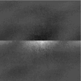
FIG. 1.: Representation wavelet $\Psi$ for the image ensemble. The function is represented in gray levels, the darkest points indicate the sites where it takes its smallest values.

III The representation mother wavelet

We suppose that the contrast field obtained from our image dataset can be expanded as a superposition of wavelets, eq.(3), and that the $\alpha_{j\vec{k}}$’s verify eq. (5), where the $\eta_{j\vec{k}}$’s are scale independent equally distributed variables. Since the images have finite size we will take $j\geq 0$ where $\Psi_{0\vec{0}}$ covers the whole image and it represents the mother wavelet, $\Psi_{0\vec{0}}\equiv\Psi$. For the same reason, the range of $\vec{k}=(k_{1},k_{2})$ at the scale $j$ is bounded as: $k_{1},k_{2}=0,1,...,2^{j}-1$.

Averaging $c(\vec{x})$ at each point $\vec{x}$, it is found that the average contrast can be represented as a simple wavelet superposition: ${\cal C}(\vec{x})\equiv\langle c\rangle(\vec{x})\propto\alpha_{0\vec{0}}\>\sum_{j,\vec{k}}{\overline{|\eta|}}^{j}\Psi_{j\vec{k}}(\vec{x})$. Here $\overline{|\eta|}$ is the first order moment of the distribution of the $|\eta|$’s, and we have used the assumptions that all the $\eta_{j\vec{k}}$’s have the same marginal distribution and are independent across the scales. By Fourier transforming this field, $\hat{\cal C}(\vec{f})$, one easily obtains the Fourier transform of the representation wavelet, $\hat{\Psi}(\vec{f})$, that reads:

$$\hat{\Psi}(\vec{f})\;=\;\frac{1}{\alpha_{0\vec{0}}}\left[\hat{\cal C}(\vec{f})-\frac{\overline{|\eta|}}{4}\;\frac{\Lambda(\vec{f})}{\Lambda(\frac{\vec{f}}{2})}\hat{\cal C}(\frac{\vec{f}}{2})\right]$$ (7)

FIG. 2.: The wavelet $\Psi$ along the horizontal (left) and the vertical axis (right).

where $\Lambda(\vec{f})=(1-e^{-2\pi if_{1}})(1-e^{-2\pi if_{2}})$. This expression is very appealing. The right hand side compares the average contrast at two consecutive scales (related by a factor $2$), and it expresses that the wavelet is obtained as an observation of the scale transformation properties of the images. The average $\overline{|\eta|}$ has an a priori known value: $\overline{|\eta|}=\frac{1}{2}$ [7]. This allows to use eq. (7) with no a priori knowledge about the data.

To obtain experimentally the representation wavelet, eq. (7) was applied to a large ensemble of natural images. The data were 200 $1024\times 1024$ images selected at random from van Hateren’s dataset [12]. Figure 1 shows the representation wavelet obtained with this procedure. It exhibits two clear features: it is right-left symmetric and roughly up-down antisymmetric with a sharp central discontinuity (see Figure 2). The first property is expected: our world remains statistically unchanged when it is reflected from left to right. The rough up-down antisymmetry and the related discontinuity are probably due to the sharp contrast between the sky and the ground.

IV The projection into the experimental basis

Once the analizer wavelet is obtained, it can be used to evaluate the coefficients $\alpha_{j\vec{k}}$ and from them, using eq. (6), the coefficients $\eta_{j\vec{k}}$. Then, it is possible to check whether the $\eta_{j\vec{k}}$ are scale-independent, identically distributed variables. In the affirmative case, this fact self-consistently demonstrates that eq. (7) is the intrinsic wavelet we are looking for. It is immediate to check that the signs of the $\eta$’s are independent of their absolute values, $|\eta|$, and also scale-independent, so it is only necessary to verify the independence of the $|\eta|$’s.

The mutual dependence among the $|\eta_{j\vec{k}}|$’s was estimated by computing the correlation coefficients between two $|\eta|$’s. As the number of possible pairs is very large, only two types of correlations were considered, which should be maximal by construction: those between consecutive scales ($j-1$ and $j$) at equivalent positions, and those between consecutive spatial positions ($\vec{k}$ and $\vec{k}+\vec{d}$, where the components of $\vec{d}$ take only the values $0$ and $1$) at a fixed scale $j$.

FIG. 3.: P.d.f.’s of $\ln|\eta_{j}|$ at the scales $j=$ 2 (diamonds), 3 (crosses), 4 (squares), 5 (x), 6 (triangles) and 7 (crossed x).

Both correlation coefficients, denoted as $\rho_{j}$ and $\rho_{j\vec{d}}$ respectively, take values in $[-1,1]$ and give a dimensionless measure of the degree of statistical dependence. The observed values of $\rho_{j}$ are very close to $0$ ($|\rho_{j}|<10^{-2},\>j>2$), what confirms rather well the independence of the $\eta_{j\vec{k}}$’s under changes of scale. On the contrary, the correlation coefficients $\rho_{j\vec{d}}$ are by no means negligible, although they are extremely short-ranged: the variables $\eta_{j\vec{k}}$ and $\eta_{j\vec{k}^{\prime}}$ are independent when they are more than one pixel apart; after that distance the two-point correlation $\rho_{j\vec{d}}$ decays dramatically. It is important to remark that there is no need of spatial independence of the $\eta_{j\vec{k}}$’s in our wavelet model. For this reason, although short-ranged, the observed dependence is a significant source of information about the remaining statistical structure at a fixed resolution layer. On the other hand, the $\eta$’s define a system of almost completely independent variables.

To confirm the validity of the wavelet representation, eqs. (3) and (7), one has still to check that the $\eta$’s are identically distributed. Figure 3 exhibits the distribution of $\ln|\eta_{j}|$ for different scales $j$. The correspondence between them is really very good.

V Wavelet transparency and decorrelation

It has been frequently argued that the the signal that arrives to the primary visual cortex has been already decorrelated in previous stages of the visual system [3, 13]. In this case, V1 would take care of coding more complex aspects of images. In this regard, the way in which the mother wavelet is constructed guarantees a remarkable property of transparency to the power spectrum: it defines a code that is somewhat independent of the second order statistics of the images. The power spectrum of natural images exhibits a power law behaviour, $S(\vec{f})\sim f^{-(2-\epsilon)}$ [2]. Under the assumption of translational invariance, the application of the decorrelating filter to the contrast is equivalent to multiplication in the Fourier domain by $f^{1-\frac{\epsilon}{2}}$. Denoting the decorrelated contrast as ${\bf D}c(\vec{x})$, it is immediate to see that it has a representation similar to eq. (3):

$${\bf D}c(\vec{x})\;=\;\sum_{j\vec{k}}\alpha_{j\vec{k}}^{\prime}\>{\bf D}\Psi_{j\vec{k}}(\vec{x})\;\;\;,$$ (8)

where ${\bf D}\Psi$ indicates the application of the decorrelating operator to the representation wavelet and $\alpha_{j\vec{k}}^{\prime}=2^{j(1-\frac{\epsilon}{2})}\alpha_{j\vec{k}}$. Defining now $\eta_{j\vec{k}}^{\prime}=2^{1-\frac{\epsilon}{2}}\eta_{j\vec{k}}$ it is concluded that the decorrelated images also posses a random multiplicative process. The new representation wavelet ${\bf D}\Psi$ can be obtained from an ensemble of decorrelated images by means of eq. (7). It is known that the value of the exponent $\epsilon$ has fluctuations from image to image [14]. The relevance of the wavelet transparency is that if the visual stimulus has been decorrelated before it reaches V1, this area can use the type of filters described in this paper regardless of the precise exponent of the power spectrum.

VI Conclusions

We have shown that images can be represented as multiresolution objects in terms of an appropriate wavelet basis $\Psi$, in which each resolution level is an independent image. One of the advantages of this representation is that it is based on the observed properties of the contrast gradient [6, 7], what in turn leads to an automatic reduction of the redundancy. At the same time the spatial correlations at a given scale are short-ranged, but still informative.

Once the wavelet is known, it is possible to devise a compression technique based on the properties of this representation. This would have two important advantages with respect to other wavelet representations (see e.g. [15]): first that the scale layers are independent, and second that there exists a simple model for the distribution of coeficcients [6, 7, 8] that can be used in the coding.

These results have been obtained with the simplest wavelet expansion, but the tools presented in this work can be taken as the starting point to look for more realistic visual filters. This search should be directed by the experimental observation that cells in V1 are edge detectors. From this perspective, the expansion in eq. (3) should be generalized to include an orientational degree of freedom. Filters of this type have been proposed in [16] and found from an independent component analysis of natural images [17] . These studies should be combined with the use of overcomplete basis, this introduces redundancy but the representation becomes stable under small changes in the images [18]

This analysis could also be carried out over any physical system with multiscaling properties, eq. (4) (for instance, turbulent flows in fully developed turbulence [11]). For all these systems eq. (7) could be applied to obtain the associated representation wavelet $\Psi$. However, it would be necessary to check the statements of scale independence and identical distribution for the projection coefficients $\eta_{j\vec{k}}$. If both properties hold, the compact code so obtained would be a valuable tool, and the interpretation of the possible remaining structure at each scale very meaningful.

Acknowledgements

This work was funded by a Spanish grant PB96-0047. A. Turiel is financially supported by a fellowship from the Spanish Ministry of Education.

REFERENCES

- [1] Barlow H. B., in Sensory Communication (ed. Rosenblith W.) pp. 217. (M.I.T. Press, Cambridge MA, 1961)
- [2] Field D. J., J. Opt. Soc. Am. 4: 2379-2394 (1987)
- [3] Atick J. J. Network 3: 213-251 (1992); van Hateren J.H. J. Comp. Physiology A 171: 157-170 (1992)
- [4] Field D. J., in Wavelets, Fractals, and Fourier Transforms. Eds. Farge M., Hunt J.C.R. & Vassilicos J.C., pp. 151-193. Clarendon Press, Oxford (1993).
- [5] Ruderman D. & Bialek W., Phys. Rev. Lett. 73: 814 (1994); Ruderman D., Network 5: 517-548 (1994)
- [6] Turiel A., Mato G., Parga N. & Nadal J.-P. Phys. Rev. Lett. 80: 1098-1101 (1998); Turiel A., Mato G., Parga N. & Nadal J.-P. Proc. of NIPS’97. MIT Press, Cambridge, MA (1998).
- [7] Turiel A. & Parga N. Neural Computation 12: 763-793 (2000)
- [8] Nevado A., Parga N & Turiel A. Network 11: 131-152 (2000); Turiel A., Parga N., Ruderman D. & Cronin T.W., To appear in Phys. Rev. E (1999); Turiel A. & del Pozo A. Sub. to IEEE Transactions on Image Processing (2000)
- [9] Buccigrossi R.W. and Simoncelli E.P., IEEE Trans Image Processing 8, 1688-1701, (1999).
- [10] Daubechies I. “Ten Lectures on Wavelets”. CBMS-NSF Series in Ap. Math. Capital City Press. Montpelier, Vermont (1992)
- [11] Frisch U., Turbulence, Cambridge Univ. Press (1995)
- [12] Hateren, J.H. van & Schaaf, A. van der Proc.R.Soc.Lond. B 265: 359-366 (1998)
- [13] Yang Dan, Atick J. & Clay Reid R., J. of Neuroscience 16: 3351-3362 (1996)
- [14] Tollhurst D. J., Tadmor Y. & Tang Chao, Ophthal. Physiol. Opt. 12: 229-232 (1992)
- [15] Said A & Pearlman W IEEE Trans Image Proc 5 1303-1310 (1996)
- [16] Daugman J.G., , IEEE Transactions on Biomedical Engineering 36: 107-114 (1989)
- [17] Bell A.J. & Sejnowski T.J., Vision Research 37: 3327-3338 (1997)
- [18] Simoncelli E.P., Freeman W.T., Adelson E.H. & Heeger D.J., IEEE Transactions on Information Theory 382: 587-607 (1992); Olshausen B.A. & Field D.J., Vision Research 37: 3311-3325 (1997)