Multiscaling and information content of natural color images

Abstract

Naive scale invariance is not a true property of natural images. Natural monochrome images posses a much richer geometrical structure, that is particularly well described in terms of multiscaling relations. This means that the pixels of a given image can be decomposed into sets, the fractal components of the image, with well-defined scaling exponents (Turiel & Parga, submitted). Here it is shown that multispectral representations of natural scenes also exhibit multiscaling properties, observing the same kind of behavior. A precise measure of the informational relevance of the fractal components is also given, and it is shown that there are important differences between the intrinsically redundant RGB system and the decorrelated one defined in (Ruderman, Cronin & Chiao, 1998).

PACS numbers: 42.66.Ne, 87.19.Db,47.53.+n,47.54.+r

Pysical Review E 62, 1138-1148 (2000)

I Introduction

The description of the early stages of the visual pathway in mammalians and other animals must be addressed from the knowledge of the properties of the signal that this system is intended to encode: natural images [1, 2, 3, 4, 5]. These are very complex objects, and truly random from the point of view of the observer. However, natural images are structured, highly redundant objects, a fact that becomes clear for instance in that the luminosity changes smoothly over the reflecting surfaces. This redundancy, which should be used as a priori knowledge about the signal, is useful to develop optimal coding strategies, which are learnt by the sensory system. It is then a crucial task to describe the redundancy. In the study of multispectral images we are faced with two kinds of redundancy: chromatic and geometrical.

The information conveyed by multispectral images is obviously very redundant, particularly for those spectral channels with the closest wavelengths. Each channel behaves statistically much like a single monochrome channel, with similar geometrical redundancies and strong mutual dependencies. Taking as starting point the usual three-channel RGB representation (that we will hereafter call the chromatic system RGB) according to the human sensory receptor classes, Ruderman et al [6] developed a chromatic system of three new variables (called $l\alpha\beta$). As defined, this chromatic system decorrelates the three signals at each point in the image. Thus, these signals define a more compact codification of the RGB images. Moreover, the variables these authors obtain are reminiscent of the chromatic channels of human color vision.

With respect to geometrical redundancy, it is a well known fact that natural images possess power law scalings which reflect their scale invariant nature. The best known of these scaling properties is the one associated with the power spectrum (see [7, 8] for instance), which is usually related to the fractal character of images. Recently, a hierarchical class of scaling laws has been observed in monochrome natural images: those forming the so called Self-Similarity (SS) and Extended Self-Similarity (ESS) properties (see [9]). This more detailed structure reveals that images are not simple fractals, but multifractal objects which can be split into different fractal sets that transform differently under changes in scale. The hierarchical structure of the fractal components has been even proposed as a natural way of classifying the information content of the visual scenes [10].

The aim of this work is to explain the chromatic systems both from the geometrical meaning of the fractal components of color images and from the evaluation of the information conveyed by each chromatic channel over the fractal components. We will present the following:

1. Verification of the scaling laws (SS and ESS) in the chromatic sytems (that is, the standard Red-Green-Blue (RGB) and the decorrelating one (l$\alpha\beta$) [6].

2. Performance of a multifractal decomposition of images for the two chromatic sytems and a classification of the resulting fractal components, emphasizing the importance and the interpretation of the most relevant of them, the Most Singular Manifold (MSM).

3. Determination of the information content and the mutual informations among the three components of a given chromatic system, for different sets of pixels (whole image, MSM and second MSM).

The paper is structured as follows: In Section II the instrumental and processing methods used in the elaboration of this work are summarized. The concepts of anomalous scaling laws (SS and ESS) and their experimental validations are given in Section III. Section IV explains the Log-Poisson model which is used to describe the anomalous exponents. In Section V our statistical results are interpreted in geometrical terms, and the decomposition of the images into their fractal components is shown. In addition, the differences between the two chromatic systems are also observed and explained. In Section VI a precise measure of the information content and mutual informations of the variables are given and interpreted. Finally, the main conclusions are presented in Section VII.

II Methods

The data gathering methods were as in [6]. Briefly, spectral images were captured using an Electrim EDC-1000TE camera with a resolution of 192 $\times$ 165 (horizontal $\times$ vertical) 8-bit pixels. Light reaching the CCD array was passed through a variable interference filter with a wavelength range of 400 to 740 nm of bandpass typically 15 nm. In each image, 43 successive images were taken of each scene at 7-8 nm intervals from 403 to 719 nm. Each pixel subtended a rectangle of $0.047\times 0.055$ degrees (horizontal $\times$ vertical). No corrections for optical or CCD-element spatial filtering were made; however the estimated dark noise was subtracted from each CCD image on a pixel-by-pixel basis. In attempting to select a diversity of typical foliage-dominated scenes, images were collected in several locations around Baltimore, Maryland (temperate woodland) and Brisbane, Australia (sclerophyll forest, subtropical rainforest, and mangrove swamp). Selected scenes contained numerous natural objects, including leaf foliage, bark, rocks, herbs, streams, bare soil, etc. In one corner of each imaged scene small reflectance standards were placed for calibration purposes: a Spectralon 100% diffuse reflectance material (Labsphere) and a nominally 3% spectrally flat diffuse reflector (MacBeth).

We collected images of 12 such natural scenes, and further analyzed the central 128 x 128 pixel region. Each of the ($128\times 128\times 12=196608$) pixels was converted to three theoretical cone responses as $\sum_{\lambda}Q(\lambda)R(\lambda)I(\lambda)$, where $Q(\lambda)$ is the Stockman-MacLeod-Johnson cone fundamental [11] for the given cone type, $R(\lambda)$ is the measured image reflectance data, $I(\lambda)$ is the standard illuminant D65 (which is meant to mimic a daylight spectrum [11, 12]), and the sum is over wavelengths represented in the spectrum. Our results depend only very weakly on the choice of illuminant, so long as it is broadband. This procedure provides the cone response data $L(\vec{x})$, $M(\vec{x})$, and $S(\vec{x})$, proportional to the number of quanta absorbed in an L, M, or S cone at spatial location $\vec{x}$ within the image. The raw reflectance data for the 12 images are available via anonymous ftp at ftp://sloan.salk.edu/pub/ruderman/hyperspectral/.

We will make use of two different chromatic systems of cone response variables to represent each image, the RGB system and the $l\alpha\beta$ system. The RGB system is formed by the raw L (Blue), M (Green) and S (Red) responses and is intended to be an unprocessed representation of the image. The $l\alpha\beta$ system is formed by the variables obtained in [6], which is defined as follows:

$$l = \frac{1}{\sqrt{3}}(\log L\>+\>\log M\>+\>\log S)\>-\>l_{0}$$ (1)

$$\alpha = \frac{1}{\sqrt{6}}(\log L\>+\>\log M\>-\>2\log S)\>-\>\alpha_{0}$$ (2)

$$\beta = \frac{1}{\sqrt{2}}(\log L\>-\>\log M)\>-\>\beta_{0}$$ (3)

where $l_{0}$, $\alpha_{0}$ and $\beta_{0}$ are appropriate constants verifying that the average of each variable over each image is equal to zero. These variables are decorrelated, that is, the average of the product of any two different variables vanishes (see [6]. This decorrelation property is a weak kind of independence (if the variables are independent then they are decorrelated).

III Statistics of images: Multiscaling

It is believed that natural images behave like ”fractal” objects: they do not possess a scale of reference and they are self-similar [7], each small portion of them behaving in the same as the whole image (in a statistical sense). However the kind of self-similar behavior shown by the power spectrum is insufficient to provide a detailed description of the local structure of natural scenes. [13, 14, 9, 10] This is because it assigns the same scaling exponent to every image pixel. To obtain a better description of the image, it is necessary to define a variable with a local scope, able to detect its local features. The hope is that a variable like this could assign distinct self-similar behaviors to different pixels, which in turn could be used to detect and classify its local features. Examples of this approach can be found in [9, 10], where dealing with grayscale images a whole hierarchy of image fetures, from sharp edges to textures, has been put in correspondence with local scaling exponents.

In this work the approach is extended to color images. The existence of a hierarchy is explored and explicitly checked for all the components of the chromatic systems presented in the previous section. In analogy with the variables defined in [9, 10], given any of the chromatic components presented in Section II, the Edge Content (EC) of this component at the point $\vec{x}$ and at the scale $r$, $\epsilon_{r}(\vec{x})$, is defined as:

$$\epsilon_{r}(\vec{x})\;=\;\frac{1}{r^{2}}\>\int_{B_{r}(\vec{x})}\mbox{$\!\!\!\!\!\!$}\mbox{$\!\!\!\!$}d\vec{x}^{\prime}\;\;\;|\nabla C|(\vec{x}^{\prime})\;\;\;,$$ (4)

where $C(\vec{x})$ denotes the selected chromatic component (e.g., R, G, B, $l$, $\alpha$ or $\beta$). The bi-dimensional integral is defined over $B_{r}(\vec{x})$, which represents a square of linear size $r$ centered at $\vec{x}$. We will often use one-dimensional surrogates of the EC, which are statistically less demanding. These are defined as integrals along a direction given by a vector $\vec{r}$ of length $r$:

$$\epsilon_{\vec{r}}(\vec{x})\;=\;\frac{1}{r}\>\int_{-r/2}^{r/2}\mbox{$\!\!\!\!\!\!$}ds\;\;|\frac{\partial C}{\partial s}(\vec{x}+s\frac{\vec{r}}{r})|$$ (5)

As noted before, these variables compute the average over a scale $r$ of a quantity that compares two neighboring points. It is then clear that even its marginal distribution contains information about the local structure of the image. This is not the case for the more usual average over the same scale of the chromatic components themselves.

We now introduce the important concepts of Self Similarity (SS) and Extended Self Similarity (ESS). Given a random variable $\epsilon_{r}$ defined on a local area of size $r$, we would say that this variable has SS if its statistical moments of order $p$ obey a power law with exponent $\tau_{p}$:

$$\langle\epsilon_{r}^{p}\rangle\;=\;\alpha_{p}\>r^{\tau_{p}}\;\;,$$ (6)

where $\alpha_{p}$ is a geometrical factor. Since $\tau_{p}$ is an arbitrary function of $p$, this is a more general type of scaling than the one observed in the power spectrum. The knowledge of an infinite collection of exponents will provide a useful description of the system. The simplest possible system exhibiting SS is that in which $\tau_{p}\propto p$. In that case, the dependence on the scale parameter $r$ is trivial: it simply implies that the moments of the normalized variable $\epsilon_{r}/\langle\epsilon_{r}\rangle$ do not depend on $r$. The most interesting cases are those in which $\tau_{p}\neq\tau_{1}\>p$, and this deviation is known as anomalous scaling.

The concept of ESS requires that the moments verify a weaker identity:

$$\langle\epsilon_{r}^{p}\rangle\;=\;A(p,2)\>\langle\epsilon_{r}^{2}\rangle^{\rho(p,2)}\;\;\;.$$ (7)

Notice that any moment of order $q$ could be used in the place of the second order one (provided $\rho(q,2)\neq 0$). If $\epsilon_{r}$ has SS it also has ESS, and the relation between the exponents $\tau_{p}$ and $\rho(p,2)$ is:

$$\rho(p,2)\;=\;\frac{\tau_{p}}{\tau_{2}}\;\;\;.$$ (8)

We can now verify if SS and ESS hold for the dataset presented in Section II. For this purpose we have used the variables $\epsilon_{\vec{r}}(\vec{x})$ (eq. (5)) taking $\vec{r}$ in both the horizontal and the vertical directions. The numerical analysis was done over the six EC variables built on the six chromatic components RGB and $l\alpha\beta$. The scale $r$ was taken small compared with the total size of the image ($r\leq 64$ pixels) and $p$ was taken up to $p=10$. It was observed that both SS and ESS hold. The test for ESS is presented for the horizontal EC of the chromatic components RGB in fig. 1 and for the chromatic components $l\alpha\beta$ in fig. 2.

The ESS exponents $\rho(p,2)$ are shown in fig. 3 , again for the three components of the two chromatic systems.

IV Multiplicative processes: Log-Poisson model

The data presented in the previous section show that ESS holds for the six chromatic components discussed in this work. We show here that a very simple model, based on a Log-Poisson multiplicative process [15, 16, 17, 9], is able to fit this data. The existence of such a process means that the EC at a scale $r$ is obtained from the EC at a greater scale $L$ by multiplying it by a random variable $\alpha_{rL}$:

$$\epsilon_{r}\;=\;\alpha_{rL}\>\epsilon_{L}$$ (9)

where $\alpha_{rL}$ is independent of $\epsilon_{L}$. The random factors $\alpha_{rL}$ define the multiplicative process, and for any intermediate scale $r^{\prime}$, $r<r^{\prime}<L$, the following relation must hold:

$$\alpha_{rL}\;=\;\alpha_{rr^{\prime}}\>\alpha_{r^{\prime}L}\;\;.$$ (10)

This implies that the process can be infinitely split into many intermediate stages, and it is thus said to be infinitely divisible. The factor $\alpha_{rL}$ takes account of the consecutive transitions of the EC from a large scale in the image to smaller ones. Knowing the process and the probability distribution of the EC at the largest scale $L$, the probability distribution of the EC at any other scale $r<L$ can be computed.

Under an infinitesimal change in the scale (when the EC at scale $r$ is generated from the EC at scale $r+dr$) the Log-Poisson model is a binomial distribution with one event infinitely less likely than the other. The most probable event corresponds to smooth transitions in the contrast (e.g., the surface of an object); whereas the infinitesimally rare event indicates a sharp transition (e.g. an edge). More precisely, the $\alpha_{rL}$’s are obtained by:

$$\alpha_{r,r+dr}=\left\{\begin{array}[]{ccc}\\ 1-\Delta\frac{dr}{r}&,&\mbox{probability: $1-[d-D_{\infty}]\frac{dr}{r}$}\\ \\ \beta(1-\Delta\frac{dr}{r})&,&\mbox{probability: $[d-D_{\infty}]\frac{dr}{r}$}\\ \\ \end{array}\right.$$ (11)

where the parameters $\Delta$ and $D_{\infty}$ can be expressed in terms of the SS exponent $\tau_{2}$ and the modulation parameter $\beta$ by (for details see [10]):

$$\left\{\begin{array}[]{ccc}\Delta&=&-\frac{\tau_{2}}{1-\beta}\\ &&\\ d-D_{\infty}&=&-\frac{\tau_{2}}{(1-\beta)^{2}}\end{array}\right.\;\;.$$ (12)

Here $d$ is the dimensionality of the system; $d=2$ for our images. When a non-infinitesimal change in scale is considered, this formula leads to a Log-Poisson distribution for the multiplicative process $\alpha_{rL}$. The probability distribution of $\alpha_{rL}$, $\rho_{\alpha_{rL}}(\alpha)$, is given by:

$$\rho_{\alpha_{rL}}(\alpha)\;=\;e^{-s_{rL}}\>\sum_{n=0}^{\infty}\frac{s_{rL}^{n}}{n!}\delta(\alpha-\beta^{n}(\frac{L}{r})^{\Delta})$$ (13)

where $s_{rL}=(d-D_{\infty})\ln\frac{L}{r}$ is the average number of modulations between the two scales. Notice that this distribution depends only on the ratio between the two scales. This model has been used previously to describe turbulent flows [18] and grayscale natural images [9, 10].

The ESS exponents $\rho(p,2)$ can be calculated from eq. (13). They depend only on the modulation parameter $\beta$:

$\displaystyle\rho(p,2)\;=\;\frac{p}{1-\beta}\>-\>\frac{1-\beta^{p}}{(1-\beta)^{2}}\;\;.$

Besides, using eq. (8) one sees that the set of SS exponents $\tau_{p}$’s can be computed with only two parameters (namely $\beta$ and $\tau_{2}$).

To conclude this section let us notice that eq. (9) allows us to compute the distribution of $\alpha_{rL}$ from the distributions of the EC’s at the scales $L$ and $r$, by deconvolution (Notice that this deconvolution problem is numerically ill-posed. As a consequence, the distribution of $\alpha_{rL}$ so obtained is less precise than the one inferred by fitting the moments of the EC.). Two examples of these distributions are shown in Figure 4, together with the Log-Poisson distribution (eq. (13)). Notice that a Log-Poisson distribution becomes eventually Log-Normal. The reason is that the infinitely divisible character of $\alpha_{rL}$, expressed in eq. (10) implies that $\ln\alpha_{rL}$ is the sum of an infinite number of independent random variables. Provided that the dispersion of that sum is small compared with its mean, this process will get closer to normal. This is not seen in Fig. 4 because at the two considered scales the average number of transitions is rather small. This is a manifestation of the fact that natural images present far-from-gaussian behavior.

V Geometry of chromatic components: the multifractal representation

The anomalous scaling laws for the moments of the chromatic EC’s can be explained on the basis of local anomalous scaling exponents. We define the Edge Measure (EM) for a given chromatic component of a square of side $r$ centered around a point $\vec{x}$, $\mu(B_{r}(\vec{x}))$, as:

$$\mu(B_{r}(\vec{x}))\;=\;r^{2}\>\epsilon_{r}(\vec{x})$$ (14)

so the EC is just a comparison between the EM of a square and its standard area $r^{2}$. The convenience of the definition of the EM with respect to that of the EC is given by the fact that the EM is additive: if for instance a square is split in several pieces, the EM of the square is the sum of the EM’s of its parts. It is natural to ask whether the EM of a square shows a local power law scaling as:

$$\mu(B_{r}(\vec{x}))\>=\>\alpha(\vec{x})\>r^{h(\vec{x})+2}\>\>,$$ (15)

where $h(\vec{x})$ is the local scaling exponent of a chromatic component at the point $\vec{x}$. It measures the strength of the singularity at this point. A measure verifying eq. (15) is said to be multifractal. The reason for this name is that any image with a multifractal measure can be arranged in fractal components, $F_{h}$. For each chromatic component, these are the sets of points with the same exponent $h$. The fractal dimension of each set will be denoted as $D(h)$ and this function is called the singularity spectrum of the multifractal.

It is a well-known fact [19] that $D(h)$ is the Legendre transform of $\tau_{p}$. This allows not only the computation of the singularity spectrum from the statistical data, but also the determination of the range of observed local singularities $h$. In the Log-Poisson model, the whole singularity spectrum is determined by only two parameters. For instance, these can be chosen as $\beta$ and $\tau_{2}$, and so it reads [18, 10]:

$$D(h)\;=\;d\>+\>\frac{\tau_{2}}{(1-\beta)^{2}}\>-\>\frac{h-\frac{\tau_{2}}{1-\beta}}{\ln\beta}\left[1-\ln\left(\frac{h-\frac{\tau_{2}}{1-\beta}}{\frac{\tau_{2}\>\ln\beta}{(1-\beta)^{2}}}\right)\right]$$ (16)

(here, $d=2$). More interestingly, they can be chosen as $\Delta$ and $D_{\infty}$. Now the singularity spectrum reads:

$$D(h)\;=\;D_{\infty}+(d-D_{\infty})w(h)[1-\ln w(h)]$$ (17)

where $\omega(h)=-(h+\Delta)/[(d-D_{\infty})\ln\left(1-\frac{\Delta}{d-D_{\infty}}\right)]$, a linear funciton of $h$. The fractal component with smallest exponent, $F_{\infty}$, is called the Most Singular Manifold (MSM). It turns out that $-\Delta$ is the exponent characterizing the MSM ($F_{\infty}\equiv F_{-\Delta}$) and $D_{\infty}\equiv D(-\Delta))$ is its dimension [9]. For example, for a Log-Poisson model with $\beta=0.5$ and $\tau_{2}=-0.25$ (which are close to the values experimentally observed in our dataset) one obtains that $\Delta=0.5$, $D_{\infty}=1.0$.

There are several ways of computing explicitly the local exponents $h(\vec{x})$ at a given pixel (which in turn gives the fractal components). The most convenient method, from the numerical point of view, is that of the wavelet transform (see [20, 21, 10]). It is based on the convolution of the EM density with an appropiate function $\Psi(\vec{x})$, the wavelet, which is resized using a scale variable $r$ to focus the convenient details at each scale. We thus define the wavelet projection $T_{\Psi}^{r}d\mu(\vec{x})$ at the point $\vec{x}$ and the scale $r$ as:

$$T_{\Psi}^{r}d\mu(\vec{x})\;=\;\int d\vec{y}\>|\nabla C|(\vec{y})\Psi_{r}(\vec{x}-\vec{y})$$ (18)

where $\Psi_{r}(\vec{x})\equiv\frac{1}{r^{2}}\Psi(\frac{\vec{x}}{r})$. It can be proven [22] that the EM verifies the multifractal scaling, eq. (15), if and only if:

$$T_{\Psi}^{r}d\mu(\vec{x})\;=\;\bar{\alpha}(\vec{x})\>r^{h(\vec{x})}$$ (19)

where $h(\vec{x})$ is the same exponent as in eq. (15) and $\bar{\alpha}(\vec{x})$ is a suitable function. This multiresolution method allows for a very good discrimination of the sets $F_{h}$; once they are abtained, their irregular (fractal) nature is clear by simple visual inspection.

Applying the theory to the data, using the previously computed values of $\tau_{2}$ and $\beta$ (Fig. 3) it is obtained that the MSM has a dimension $D_{\infty}\approx 1$, that is, it consists of segments of curves. Visual inspection of this set (Figures 5 and 6) reveals that it is rather close to the edges present in the chromatic components.

Comparison of the MSM’s of the two chromatic systems, RGB and $l\alpha\beta$, shows that they have qualitatively different geometrical contents. Figures 5 and 6 exemplify the question on a representative image.

• The RGB system is highly geometrically redundant. Simple visual inspection of the gray level reprentations of the three chromatic variables (first row of figure 5) shows three very similar scenes. This fact is confirmed by the multiresolution analysis (second row of figure 5).

  To characterize this geometrical redundancy, we measured the relative density of the different MSM’s and of their intersection across the whole ensemble. The values obtained are: Red MSM: 29.95%; Green MSM: 29.89%; Blue MSM: 23.75%. The relative density of the intersection of the three sets is 19.60%. This means that the intersection contains 65.44% of the Red MSM, 65.57% of the Green MSM and 82.53% of the Blue MSM, so it is clear that the three MSM share a significant amount of geometrical content. In other words: the luminosity edges typically co-occur in all the three chromatic components in this representation.

• The $l\alpha\beta$ system has significant geometrical differences among its chromatic variables. There are very well defined borders that are shared by all the variables; however, several geometrical structures are apparent only in one of the three chromatic components of the image. It seems that this representation could enhance the separation of different types of objects attending to their color distribution. This result seems very appealing. We computed again the densities of the different sets (each MSM and the intersection of the three) across the whole ensemble of images. The values are the following: $l$ MSM: 40.96%; $\alpha$ MSM: 45.30% $\beta$ MSM: 44.65%. The set resulting of the intersection of the three has a density of 13.93%, which means that it contains 34.01% of the $l$ MSM, 30.75% of the $\alpha$ MSM and 31.20% of the $\beta$ MSM. In this sense, these chromatic variables posses less geometrical redundancy than those in the RGB system. This is explained by the fact that there are sharp edges which belong just to one of the spaces and not to the other two, in contrast with the situation of the RGB system.

The inspection of these results reveals two interesting features: first, the MSM’s associated to the $l\alpha\beta$ system are denser than those of RGB system. This is mainly caused by the logarithmic transformation from RGB to $l\alpha\beta$, which increases the contrast on average and so enhances details. Second, for the $l\alpha\beta$ system, the ratio between the number of pixels in the intersection and in each of the MSM’s is less than half of the same ratio in the RGB system. This makes more evident the appearance of different geometrical structures. The higher degree of independence in the $l\alpha\beta$ system is rather natural because of their construction: they are decorrelated variables (see [6])

VI Information content

The classification of the points in the images according their multifractal structure has revealed significative differences between the RGB and the $l\alpha\beta$ schemes. Although the geometrical coincidences and the separation of features seem very informative, it is convenient to have a more quantitative criterion than the rather coarse density estimation. In particular, it would be desirable to characterize the amount of information conveyed by the MSM’s and the degree of redundancy among them. This characterization can be done by using the concepts of entropy and mutual information.

Given a random variable $X$ with a probability distribution $\mbox{$\rho_{{}_{{}_{\!\!X}}}$}(x)$, its entropy (or total information) $H_{X}$ is defined as:

$$H_{X}\;=\;-\int dx\;\mbox{$\rho_{{}_{{}_{\!\!X}}}$}(x)\log_{b}\mbox{$\rho_{{}_{{}_{\!\!X}}}$}(x)$$ (20)

It has no actual units, but depending on the basis $b$ of the logarithm a unit name is usually given. For $b=2$, which we will use, it is expressed in bits. For discrete variables this quantity is always a finite, positive number, which is maximum for uniformly distributed variables. For continuous variables it does not even need to be defined, and can have a positive or negative value. For this reason, when a discretization of a continuous variable is considered the discretization range is very relevant. It can be proved (see for instance [23]) that for discretized variables the entropy represents an optimal bound for the average amount of digits to be used in the encoding of events described by $X$.

Given two random variables, $X$ and $Y$, with marginal probability distributions $\mbox{$\rho_{{}_{{}_{\!\!X}}}$}(x)$ and $\mbox{$\rho_{{}_{{}_{\!\!Y}}}$}(y)$ and joint probability distribution $\mbox{$\rho_{{}_{{}_{\!\!X\!Y}}}$}(x,y)$, we define the mutual information between $X$ and $Y$, $I_{X\!Y}$, as:

$$I_{XY}\;=\;\int dx\int dy\;\mbox{$\rho_{{}_{{}_{\!\!X\!Y}}}$}(x,y)\>\log_{b}\frac{\mbox{$\rho_{{}_{{}_{\!\!X\!Y}}}$}(x,y)}{\mbox{$\rho_{{}_{{}_{\!\!X}}}$}(x)\mbox{$\rho_{{}_{{}_{\!\!Y}}}$}(y)}$$ (21)

It is expressed in the same units as the entropy. It can be proved that it is always a positive quantity which only vanishes when $\mbox{$\rho_{{}_{{}_{\!\!X\!Y}}}$}(x,y)=\mbox{$\rho_{{}_{{}_{\!\!X}}}$}(x)\mbox{$\rho_{{}_{{}_{\!\!Y}}}$}(y)$, so in a sense it is a measure of the statistical independence of the variables $X$ and $Y$. In fact, it gives the amount of information shared by the two variables:

$$I_{XY}\;=\;H_{X}\>-\>H_{X|Y}\;=\;H_{Y}\>-\>H_{Y|X}$$ (22)

where $H_{X|Y}$ is the conditional entropy, defined as:

$$H_{X|Y}\;\equiv\;\int dy\;\mbox{$\rho_{{}_{{}_{\!\!Y}}}$}(y)\>[-\int dx\>\mbox{$\rho_{{}_{{}_{\!\!X|Y}}}$}(x|y)\log_{b}\mbox{$\rho_{{}_{{}_{\!\!X|Y}}}$}(x|y)]$$ (23)

and $\mbox{$\rho_{{}_{{}_{\!\!X|Y}}}$}(x|y)=\mbox{$\rho_{{}_{{}_{\!\!XY}}}$}(x,y)/\mbox{$\rho_{{}_{{}_{\!\!Y}}}$}(y)$ is the distribution of $X$ conditioned by $Y$. The conditional entropy is the average of the entropy of $X$ for fixed values of $Y$. It is the part of the entropy of $X$ which is independent of $Y$: $0<H_{X|Y}\leq H_{X}$ and $H_{X|Y}=H_{X}$ only if $X$ is independent of $Y$. Thus, the mutual information, according to eq. (22), measures the amount of bits of $X$ which can be predicted by the knowledge of $Y$ and vice-versa.

The definition of mutual information can be extended to more than two variables, although not in a unique way. We will work with the information shared by three variables $X$, $Y$ and $Z$, which can be expressed as:

$$I_{XYZ}\;=\;I_{XY}\>-\>I_{XY|Z}$$ (24)

where $I_{XY|Z}$ is the averaged mutual information between $X$ and $Y$ for fixed values of $Z$ (that is, it is computed using $\mbox{$\rho_{{}_{{}_{\!\!XY|Z}}}$}(x,y|z)$). The interpretation of this quantity is similar to that of eq. (22). The last term is the amount of information between $X$ and $Y$ which is not shared by $Z$, while the difference gives the information shared by the three variables. Contrary to the mutual information of two variables (eq. (22)), which is always positive, $I_{XYZ}$ can be negative. This happens when fixing the value of $Z$ causes the relation between $X$ and $Y$ to become less random, increasing their statistical dependence. As an extreme case we consider $X=Y+Z$, with $Z$ independent of $Y$. Fixing $Z$, the quantity $I_{XY|Z}$ takes its maximum value $H_{Y}$, and $I_{XYZ}=-H_{Y|X}$. On the other hand, a positive value of $I_{XYZ}$ indicates that fixing $Z$ the other two variables become more independent.

It can be proved that:

$$I_{XYZ}\;=\;I_{YZ}\>-\>I_{YZ|X}\;=\;I_{XZ}\>-\>I_{XZ|Y}$$ (25)

that is, the difference between the two mutual informations is independent of which variable is kept fixed. An explicitly symmetric expression is given by:

$$I_{XYZ}\;=\;I_{XY}\>+\>I_{XZ}\>+\>I_{YZ}\>-\>K_{XYZ}$$ (26)

where

$$K_{XYZ}\;=\;\int dx\int dy\int dz\;\mbox{$\rho_{{}_{{}_{\!\!X\!Y\!\!Z}}}$}(x,y,z)\>\log_{b}\frac{\mbox{$\rho_{{}_{{}_{\!\!X\!Y\!\!Z}}}$}(x,y,z)}{\mbox{$\rho_{{}_{{}_{\!\!X}}}$}(x)\mbox{$\rho_{{}_{{}_{\!\!Y}}}$}(y)\mbox{$\rho_{{}_{{}_{\!\!Z}}}$}(z)}$$ (27)

We now start the information analysis of the multifractal densities $|\nabla C|(\vec{x})$ of the chromatic components, when the point $\vec{x}$ runs across particular geometrical sets. We are interested in measuring entropies and mutual informations among the three variables of each chromatic system, at the same pixel $\vec{x}$, averaging over all the pixels of the image ensemble.

For each chromatic system we consider three different geometrical sets. The first is obtained from the whole images; the second contains the pixels common to the MSM’s of the three components; and the third is given by the pixels common to the second MSM’s. The comparison between these sets will give valuable knowledge about the distribution of information in the image.

We obtained the following results:

• RGB system: The results are summarized in Table I.

  It is observed that the entropic content of the MSM is larger than that of the whole image, while for the following manifold this entropic increase is not present: this means that the MSM is the most informative fractal component. Besides, comparing the entropy of the second MSM with that of the whole image, it is seen that they are similar (again, the lack of contrast in the Blue component causes that some of the pixels in the MSM are detected as belonging to the second MSM). This implies that sampling pixels in the second MSM gives the same information as sampling in the whole image (it was also observed that less singular fractal components give the same information as the whole image). This system exhibits a rather large amount of mutual information between pairs of variables, which is maximal for the pair Red-Green (those with the most similar wavelength ranges) for the three geometrical sets. Related to this, one also observes that $I_{GB}\simeq I_{RB}\simeq I_{RGB}$, that is the information shared by the pairs GB or RB is close to the information common to the three variables. This shows again the strong dependence between the Red and Green components.

  Notice that the mutual informations also follow the same changes shown by the entropies over the geometrical sets.

• ${\bf l\alpha\beta}$ system: Table II summarizes the results obtained for this system.

  We first notice that all the entropies are larger than those of the RGB components. It also exhibits an entropic increment of the MSM with respect to the whole images, although it is smaller than for the RGB system. Again the entropies defined over the second MSM are rather similar to those of the whole image.

  The two-variable mutual informations are rather small, which is expected because of the decorrelation achieved by this system. Contrary to the RGB system, now $I_{l\alpha\beta}<0$, which yields an increase of the mutual information between two variables when the third is known. Let us emphasize that on the pixels common to the three MSM’s the value of $I_{l\alpha\beta}$ is still more negative: this implies that on this set the degree of dependence of the gradients is larger than over the whole image. Given that in this system the three two-variable mutual informations are rather close, the argument applies to the three possible pairs.

VII Conclusions

In this work we have studied the statistical properties of spatial changes of the chromatic channels in two different chromatic systems: the cone responses RGB and the decorrelated version of these, $l\alpha\beta$ [6]. The main conclusion is that natural color images exhibit multiscaling effects similar to monochromatic images [9, 10], for both chromatic systems. In particular, it has been checked that the multiscaling statistical properties are very well described in the context of multiplicative processess, with just two free parameters.

An explicit decomposition of the images in their fractal components was also done using a wavelet technique. The most important of these components (that we have called the Most Singular Manifold, MSM), is given by the obvious contours in each chromatic channel. It was found that the RGB and the $l\alpha\beta$ systems have rather different geometrical structure. While the first exhibits a great deal of redundancy, in the sense that the fractal components of the three channels are quite similar, the decorrelated system extracts different features in the different channels.

In addition to this, this fractal structure helps to detect the most informative pixels in the images. To study this issue we have computed several information quantities: the total entropy, the mutual information between pairs of channels, and the information shared by the three channels of a given system. This analysis reveals that the MSM contains the most informative pixels in the image, for the six considered channels. There are differences between the RGB and the $l\alpha\beta$ systems. All the measured quantities show that the first is highly redundant, in that a given channel contains a large amount of information about the others. On the contrary, the decorrelated system has eliminated some redundancy. However, there is still a substantial amount mutual information, which is maximal over the MSM.

We want to emphasize that the multiscaling properties discussed here give an a priori information about what a natural image is, reducing the entropy of the ensemble of natural scenes. This could be useful for explaining the processing of color images in the early stages of the visual pathway. The existence of such a rich structure suggests that the second order statistics alone do not contain all visually significant information, and that higher order centers of visual processing may be present in biological system.

Information in the RGB system
$H_{R}$ $H_{G}$ $H_{B}$ $I_{GB}$ $I_{RB}$ $I_{RG}$ $K_{RGB}$ $I_{RGB}$ Whole Image 4.77 4.78 4.13 0.94 0.90 2.76 3.76 0.84 $F_{\infty}$ 5.35 5.34 4.69 1.30 1.25 3.22 4.64 1.13 $F_{h_{1}}$ 4.92 4.93 4.73 0.86 0.81 2.78 3.72 0.73

TABLE I.: Entropies and mutual informations in the RGB system, arranged in columns. The first three columns represent the entropies of the Red, Green and Blue variables. The next three columns represent the mutual information between the different pairs. The last two columns represents the two definions we have given for the mutual information of the three variables altogether. The rows refer to the spatial extent of the sampling: the whole image (top), the intersection of the three MSM’s (middle) and the intersection of the three first manifolds (bottom); here, $h_{1}=-0.3\pm 0.1$. All the data is expressed in bits. The bit depth of $|\nabla C|(\vec{x})$ for each component was taken to be 8 bits, what means that it has been discretized in $2^{8}\equiv 256$ values; thus the maximal possible value of each entropy is 8.

Information in the $l\alpha\beta$ system
$H_{l}$ $H_{\alpha}$ $H_{\beta}$ $I_{l\alpha}$ $I_{l\beta}$ $I_{\alpha\beta}$ $K_{l\alpha\beta}$ $I_{l\alpha\beta}$ Whole Image 6.45 5.84 5.25 0.15 0.13 0.10 0.67 -0.29 $F_{\infty}$ 6.48 6.04 5.60 0.29 0.24 0.19 1.71 -0.99 $F_{h_{1}}$ 6.44 5.85 5.22 0.19 0.15 0.13 0.97 -0.50

TABLE II.: Entropies and mutual informations for the $l\alpha\beta$ system, arranged in columns. The first three columns represent the entropies for the $l$, $\alpha$ and $\beta$ variables, and the following are arranged as those of Table I. The rows refer to the same geometrical sets as in Table I. All the data is expressed in bits. The bit depth for each component was taken to be 8 bits.

$\ln\langle\epsilon_{r}^{3}\rangle$            $\ln\langle\epsilon_{r}^{4}\rangle$           $\ln\langle\epsilon_{r}^{2}\rangle$                                                                $\ln\langle\epsilon_{r}^{2}\rangle$

FIG. 1.: Verification of ESS for the third and fourth order moments of the horizontal EC in the RGB chromatic system (Diamonds:Red, crosses:Green, boxes: Blue). The best linear fits are also represented. Each data point corresponds to a fixed value of $r$, from $4$ to $64$ pixels. Although not shown here, the vertical EC gives an equally good fit.

$\ln\langle\epsilon_{r}^{3}\rangle$            $\ln\langle\epsilon_{r}^{4}\rangle$           $\ln\langle\epsilon_{r}^{2}\rangle$                                                                $\ln\langle\epsilon_{r}^{2}\rangle$

FIG. 2.: Verification of ESS for the third and fourth order moments of the horizontal EC in the $l\alpha\beta$ system. (Diamonds: $l$, crosses: $\alpha$, boxes: $\beta$). The best linear fits are also represented. It is observed that the $\beta$ component (boxes) deviates significantly from the others, probably because this component lacks numerical accuracy (it is given by the difference between the color channels with the nearest wavelengths). Each data point corresponds to a fixed value of $r$, from $4$ to $64$ pixels. Although not shown here, the vertical EC gives an equally good fit.

$\rho(p,2)$          $RGB$                                                        $l\alpha\beta$          $p$                                                            $p$

FIG. 3.: ESS coefficients $\rho(p,2)$ for the $RGB$ (left) and the $l\alpha\beta$ (right) chromatic systems, and the horizontal EC (Symbols as in Figures 1 and 2). The comparison with the Log-Poisson model prediction (as described in Section IV) is also represented for each component. RGB system: $\beta_{R}=0.45$, $\beta_{G}=0.45$ and $\beta_{B}=0.46$; $l\alpha\beta$ system: $\beta_{l}=0.50$, $\beta_{\alpha}=0.50$ and $\beta_{\beta}=0.73$

$\rho_{{}_{{}_{\!\!\ln\alpha_{rL}}}}$ a                              $\rho_{{}_{{}_{\!\!\ln\alpha_{rL}}}}$                          b

     

$\ln\alpha_{rL}$                                                                $\ln\alpha_{rL}$

FIG. 4.: Experimental distributions (diamonds) of $\ln\alpha_{rL}$ for a) the horizontal Red EC and b) the horizontal $l$ EC; $r=4$ pixels, $L=64$ pixels. Both distributions are far from Gaussian, but very close to a Poisson distribution with the appropriate parameters (crosses). The average number of transitions ($\beta$-modulations) for both processes is the same: $s=(d-D_{\infty})\ln\frac{L}{r}=2.77$. This number is rather small to yield a Gaussian behaviour

$R$                                       $G$                                       $B$

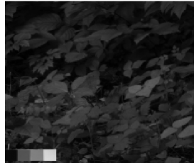
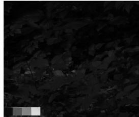
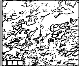
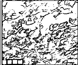
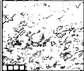
FIG. 5.: Gray level representations of the RGB system (top) and the associated MSM’s (bottom) on Park2 image. The MSM’s were taken as the sets of points having exponent $h=-0.5\pm 0.1$. The Blue component has significantly less contrast than the others, which makes it difficult or even impossible to detect some of its edges. The MSM’s of all members in the RGB system are however very similar.

$l$                                       $\alpha$                                       $\beta$

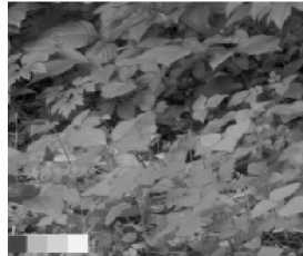
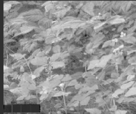
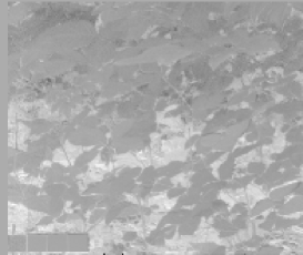
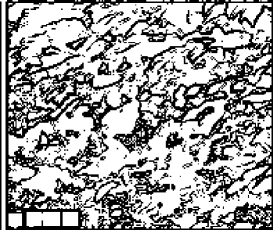
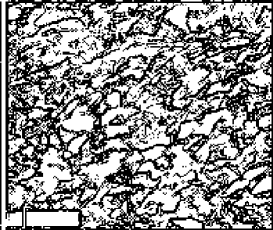
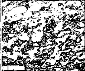
FIG. 6.: Gray level representations of the $l\alpha\beta$ system (top) and the associated MSM’s (bottom) of the Park2 image. The MSM’s were taken as the sets of points having exponent $h=-0.5\pm 0.1$. The $\beta$ component appears rather saturated. Although the most important transitions are present in the three chromatic variables, there is a significant amount of structure detected by only one of the three, reducing the geometrical redundancy.

REFERENCES

- [1] H.B. Barlow, “Possible principles underlying the transformation of sensory messages”. In Sensory Communication (ed. W. Rosenblith ) pp. 217. (M.I.T. Press, Cambridge MA, 1961).
- [2] S.B. Laughlin, “A simple coding procedure enhances a neuron’s information capacity”, Z. Naturf. 36 910-912 (1981).
- [3] J.H. van Hateren, “Theoretical predictions of spatiotemporal receptive fields of fly LMCs, and experimental validation”, J. Comp. Physiology A 171 157-170 (1992).
- [4] J.J. Atick, “Could information theory provide an ecological theory of sensory processing” ,Network 3 213-251 (1992).
- [5] J.J. Atick., Z. Li & A.N. Redlich, “Understanding retinal color coding from first principles”, Neural Computation 4 559-572 (1992).
- [6] D. Ruderman, T. Cronin & C.C. Chiao , “Statistics of cone responses to natural images: Implications for visual coding”, J. Opt. Soc. Am. A. 15, 2036-2045 (1998).
- [7] D.J. Field, “Relations between the statistics of natural images and the response properties of cortical cells”, J. Opt. Soc. Am. 4 2379-2394 (1987).
- [8] G.J. Burton & I.R. Moorhead , “Color and spatial structure in natural scenes”, Applied Optics 26 157-170 (1987).
- [9] A. Turiel , G. Mato , N. Parga & J.-P. Nadal, “The self-similarity properties of natural images resemble those of turbulent flow”, Phys. Rev. Lett. 80, 1098-1101 (1998)
- [10] A. Turiel & N. Parga, “The multi-fractal structure of contrast changes in natural images: from sharp edges to textures”, Submitted to Neural Computation (1998).
- [11] A. Stockman , D. I. A. MacLeod and N. E. Johnson, “Spectral sensitivities of the human cones”, J. Opt. Soc. Am. A, 10, 2491-2521, 1993.
- [12] G. Wyszecki & W. S. Stiles, “Color Sciences: Concepts and Methods, Quantitative Data and Formulae”. John Wiley & Sons, 2nd Edition, 1982
- [13] D. Ruderman & W. Bialek, “Statistics of natural images: scaling in the woods”, Phys. Rev. Lett. 73, 814 (1994)
- [14] D. Ruderman, “The statistics of natural images”, Network 5, 517-548 (1994)
- [15] E. A. Novikov, “Infinitely divisible distributions in turbulence”, Phys. Rev. E 50, R3303 (1994)
- [16] B. Dubrulle , “Intermittency in fully developed turbulence: Log-Poisson statistics and generalized scale covariance”, Phys. Rev. Lett. 73 959-962 (1994)
- [17] B. Castaing, “The temperature of Turbulent Flows”, J. Physique II, France 6, 105-114 (1996)
- [18] Z.-S. She & E. Leveque, “Universal Scaling laws in Fully Developed Turbulence”, Phys. Rev. Lett. 72, 336-339 (1994).
- [19] G. Parisi & U. Frisch, in Turbulence and Predictability in Geophysical Fluid Dynamics (eds Ghil M., Benzi R. & Parisi G.) 84-87 (Proc. Intl. School of Physics E. Fermi, North Holland, Amsterdam, 1985)
- [20] A. Arneodo et al. “Ondelettes, multifractales et turbulence”. Diderot Editeur. Paris (1995).
- [21] S. Mallat & S. Zhong “Wavelet transform Maxima and multiscale edges”. In “Wavelets and their applications”, Jones and Bartlett Publishers. Boston 1991.
- [22] A. Arneodo et al. “Wavelet analysis of fractals: from the mathematical concepts to experimental reality”. in Wavelets. Theory and applications (eds. Erlebacher G., Yousuff Hussaini M. and Jameson L.M.) pp. 349. (Oxford University Press. ICASE/LaRC Series in Computational Science and Engineering. 1996).
- [23] T. M. Cover & J. A. Thomas, “Elements of Information Theory”. John Wiley & Sons. New York, 1991.