Unstable decay and state selection

Abstract

The decay of unstable states when several metastable states are available for occupation is investigated using path-integral techniques. Specifically, a method is described which allows the probabilities with which the metastable states are occupied to be calculated by finding optimal paths, and fluctuations about them, in the weak noise limit. The method is illustrated on a system described by two coupled Langevin equations, which are found in the study of instabilities in fluid dynamics and superconductivity. The problem involves a subtle interplay between non-linearities and noise, and a naive approximation scheme which does not take this into account is shown to be unsatisfactory. The use of optimal paths is briefly reviewed and then applied to finding the conditional probability of ending up in one of the metastable states, having begun in the unstable state. There are several aspects of the calculation which distinguish it from most others involving optimal paths: (i) the paths do not begin and end on an attractor, and moreover, the final point is to a large extent arbitrary, (ii) the interplay between the fluctuations and the leading order contribution are at the heart of the method, and (iii) the final result involves quantities which are not exponentially small in the noise strength. This final result, which gives the probability of a particular state being selected in terms of the parameters of the dynamics, is remarkably simple and agrees well with the results of numerical simulations. The method should be applicable to similar problems in a number of other areas such as state selection in lasers, activationless chemical reactions and population dynamics in fluctuating environments.

PACS Numbers: 05.40.Ca, 05.10.Gg, 05.65.+b

I Introduction

The decay of metastable states, due to thermal or other random fluctuations, is a phenomenon seen in many diverse areas of science, and consequently has a huge literature associated with it. In the simplest cases, where a potential can be defined and the states assigned a particular value of this potential, the decay process can be viewed as noise activation over the potential barriers that separate the metastable state under consideration from all of the other accessible metastable states of the system. The average time taken to escape from a potential well (i.e. for the state to decay) is of the order of $\exp{\Delta V/D}$, where $\Delta V$ is the height of the barrier to be surmounted and $D$ is the strength of the noise. Thus the picture we have in this case, is of a set of metastable states, with transitions between them which occur with probabilities which depend on the nature of the potential between the states and on the strength of the noise.

By contrast, the decay of unstable states, although a similarly widespread phenomenon, has been studied much less. In terms of the above picture, the system starts at or near a maximum of the potential and makes transitions to the accessible metastable states of the system with various probabilities, which as before depend on the nature of the potential between the unstable and metastable states and on the noise. In an earlier paper[1] we introduced a scheme which enabled us to calculate the probabilities with which the various metastable states are selected. Our aim here is to extend this work, by giving a fuller presentation of the ideas and techniques involved, justifying some of the earlier approximations which were made and discussing the link with real systems in more detail.

The phenomenon of the selection of metastable states, from states which have become unstable, is at the heart of pattern formation and the origin of complex structures, with the selection of non-trivial states being governed partly by the deterministic dynamics and partly by the noise acting on the system. Thus the picture painted above, while a simplified version of this general scenario, contains many of its essential features. In fact, the above structure can be derived from the equations describing the entire system by focusing on the unstable modes and the modes which have the potential to be selected, and treating all of the other modes as background noise. The resulting dynamics then comprises a small number of coupled ordinary differential equations acted on by noise. If this flow is potential, then the above picture is recovered; if not, our techniques are still applicable, but it becomes more difficult to visualize.

State selection of the kind we have been describing is ubiquitous. In fluid dynamics, it appears when Rayleigh-Bénard convection rolls of given wavenumber are formed after the decay of unstable ones. A set of equations describing the non-linear coupling between parallel rolls of different wave numbers may be derived[2], and when the effects of the other modes are incorporated[3], a set of coupled stochastic differential equations of the kind mentioned above are generated. In superconductivity, exactly the same equations as in the above example govern state selection in, for example, narrow superconducting rings. This is simply because the amplitude equation which governs the instabilities in the fluid dynamics example is nothing but the Ginzburg-Landau equation for a superconductor[4]. A mode truncation then gives exactly the same set of coupled differential equations acted upon by noise[5]. In chemical kinetics, it has become clear in the last decade or two, that there are many important chemical reactions in which a barrier to the formation of an excited state is not present. Examples of these activationless reactions[6] are the electronic relaxation of triphenylmethane dyes and barrierless electron transfer in solution. The potential discussed above is a reaction potential energy surface in this case[7]. In lasers, such as the ring dye laser[8], decay of an unstable mode to metastable ones can occur under the right operating conditions. The coordinates in this case are the mode amplitudes and Langevin-type equations are derived within the semiclassical theory of the laser[9]. In population dynamics, the Gause model of two competing species[10] again falls into this class. When the competition is played out with a fluctuating environment, the resulting stochastic differential equations once again fall into the generic class that we have been discussing[11]. It should, however, be noted that in this case there is no potential and moreover the noise is multiplicative.

Although many of these phenomena have been known for some time, the investigation of the state selection aspect has been hampered by the lack of a suitable calculational tool. In the case where a potential $V$ exists, the noise is additive and only two modes, $x$ and $y$, are considered, the equations take the form

$$\dot{x} = -\frac{\partial V}{\partial x}+\eta_{x}(t)$$ (1)

$$\dot{y} = -\frac{\partial V}{\partial y}+\eta_{y}(t)\,,$$ (2)

where $\eta_{x}$ and $\eta_{y}$ are white noises of strength $D$. But, even in this, the simplest non-trivial case, these equations are difficult to study mainly because, as we shall discuss later, in the region where state selection occurs, the coupled nature of the equations, their non-linearity and the noise, are all important. However, as we have shown[1], there is a method that can take all these aspects into account, and that is the path-integral formulation of stochastic dynamics. This method succeeds where others fail because the equations can be represented as a path-integral without approximation; systematic approximation techniques for path-integrals developed over the years can then be used as the basis of a calculational scheme.

Most of the previous theoretical work on this problem has been limited to systems with one degree of freedom, governed by the single equation $\dot{x}=-V^{\prime}(x)+\eta(t)$, because many of the complexities mentioned above are not present in this one-dimensional case. Suzuki and co-workers developed a theory for the decay of an unstable state in one dimension in a series of papers[12], as did a number of other authors[13, 14, 15, 16, 17, 18, 19]. However, the one-dimensional theory, although much easier to deal with, has none of the subtleties inherent in state-selection in higher dimensions: the decay is simply either to the right or to the left. Some studies[20, 21, 22] purported to go beyond one dimension, but in fact considered spherically symmetric potentials, so that the problem could be reduced to a quasi-one-dimensional problem in the radial coordinate. Once again, the resultant structure is not rich enough to address the question of state selection. Other approaches, such as replacing the stochastic differential equations by the corresponding deterministic equations, but with random initial conditions[23], are unsatisfactory in other ways. Probably the investigation nearest to our own has been by Mangel[24], however his main interest was not state selection.

The plan of the paper is as follows. In Sec. II we discuss the assumptions underlying the picture of state selection which we have outlined and introduce a generic model which we use to describe our calculational scheme in detail. An important aspect of our method is the realization that, typically, a state is selected well before the system reaches this chosen state. This fact is used to simplify the problem in Sec. III, where it is also shown that naive calculational prescriptions, based on linearization of the initial dynamics, fail. A more systematic approach based on path-integral techniques is introduced in Sec. IV and the relevant optimal path is determined. This gives the leading order contribution in the limit $D\rightarrow 0$. The next to leading order contributions are determined in Sec. V. The results of this analytic approach are given and compared to Monte Carlo simulations in Sec. VI and our conclusions are presented in Sec. VII. There are two appendixes. Appendix A describes some of the elementary approaches described in Sec. III in more detail. Appendix B contains technical aspects relating to the determination of the $y$-coordinate of the optimal path and the calculation of the action of that path.

II General concepts

We have already given several examples of situations where state selection, following the decay of an unstable state, occurs. In this section we will explore the different ways in which the initial state of the system could arise, that is, the origin of the unstable state, and give an intuitive description of the decay and subsequent state selection, which will form the basis of our analytical approach.

An unstable state may arise by mechanisms which are either non-adiabatic or adiabatic. In the non-adiabatic case, the system, in an initially (meta)stable state, is transported very rapidly to an unstable state. The time scale for the transition from the stable to unstable state is much more rapid than the characteristic time scale defining the natural dynamics of the system. In this context the transition from the stable to the unstable state can be ignored and we simply characterize the system as having been prepared in an unstable state. Examples of this type were mentioned in Sec. I and include chemical reactions with no activation barrier and population dynamics in a fluctuating environment. Quasi-one dimensional superconductors[5] are another example. In the case of the chemical reactions, an ultra-fast light pulse (a femtosecond laser) pumps molecules into an excited state. In terms of potential surfaces, the molecules are initialized in an unstable state on the reactive surface. The subsequent reaction can be viewed as a nuclear rearrangement on this reactive potential energy surface. The evolution of the reaction, that is the relative preponderance of reactants and products, can be studied using other ultrafast lasers. In the population dynamics example, the population is initialized so as to consist of only a few individuals of each species. During the initial period the population of both species grow exponentially, independently of the other, until competition drives the population of one of the species to zero.

In the adiabatic case, an unstable state may arise when a (meta)stable state is transported through the instability over a time scale that is slow compared to the time scale characterizing the natural dynamics of the system. An example of this process is provided by a quasi one-dimensional superconductor as studied in Ref.[25]. In this case, the system is driven by a voltage source that accelerates the supercurrent. However, this acceleration cannot continue indefinitely and the system becomes unstable, a situation associated with the critical current of the superconductor. Once unstable, the relaxation process occurs via “phase slips” in which spatially localized regions of the wire temporarily lose their superconducting properties and carry “normal”, i.e. non-superconducting, current. This process dissipates the excess energy and the system relaxes back to a locally stable state. Mesoscopic wires, i.e. wires that are not in the thermodynamic limit, have a finite number of discrete metastable stationary current carrying states. State selection in this case is characterized by the competition between these metastable current carrying states. The superconductivity instability described above is an example of the Eckhaus instability.

Eckhaus instabilities arise in many physical systems in addition to quasi one-dimensional superconductors, including fluids, nematic liquid crystals and lasers. In these systems, stationary one-dimensional periodic patterns are stable for a range of wave vectors, $Q$. For instance, in the case of the common Eckhaus instability, stationary solutions exist for $Q^{2}<1$, but are only stable if $Q^{2}<1/3$. By changing the control parameter slightly, $Q$-states with $Q^{2}<1/3$ may be shifted into the unstable $Q^{2}>1/3$ regime. The essential features of the subsequent changes which follow from this may be understood by performing a mode-decomposition of the relevant amplitude equation and keeping only the previously stable mode and the destabilizing modes with the largest growth rates[5].An adiabatic elimination of the unstable mode then leaves us with coupled ordinary differential equations for the amplitudes of the destabilizing modes. This adiabatic assumption is equivalent to assuming that the form of these differential equations does not change on the time-scale of state selection, i.e. in the time taken for one of the destabilizing modes to outcompete the others[25]

An obvious question which now arises is the following: how do we know that the system is initialized in a state where the amplitudes of the competing modes, final products, etc are zero? Or expressed in the topographical terminology of Sec. I: How do we know that we begin exactly at the top of the hill? Here we are assuming that the small non-zero amplitude, required to initiate the growth, is induced by fluctuations i.e. by the noise. Once again, there are several possibilities. It may be that in every realization of the stochastic process the system starts near, but not necessarily at the origin. As long as there is no bias favoring any one of the competing modes, an average over many realizations of the process will give the same results as if the system had started at the origin in each case. Alternatively, the initial probability distribution may be so sharply peaked about the origin, that any small initial bias is irrelevant to the ultimate choice of state made by the system. Yet another possibility is that it is just not possible to start exactly at the origin (the example taken from population dynamics is a illustration of this). In these cases the sensitivity of the final result to changes in the initial starting point will have to be carefully investigated. In addition to all of these specific reasons, on general grounds beginning at the origin seems very natural, since it simply means that none of the final products or final modes are initially present.

Since there appear to be good reasons to initialize the system at the origin in many cases, it will be assumed in the subsequent theoretical development. In all of the examples given in Sec. I, the competing modes grow exponentially for an initial period, without any significant interaction with each other. This corresponds to a linear growth law of the form $\dot{x}_{l}=\alpha_{l}x_{l}$, where $x_{l}$ is the amplitude and $\alpha_{l}$ the growth rate of the $l$th mode. Clearly, the main interest from a state-selection point of view, is in the nature of the non-linear interaction terms between the modes. Since the purpose of this paper is to give a clear and intuitive introduction to our calculational scheme, we shall choose to illustrate our method on an example where only two competing modes are present, and where the interaction terms may be derived from a potential. In other words, the governing equations will have the form (2). Obviously, two is the minimum number of modes we need in order to discuss state selection, but having only two modes moving on a potential surface has the advantage that we can describe our method using the pictorial language of “hills and valleys” which we have already adopted on several occasions. Furthermore, since as we have already mentioned, the equations derived in both the fluid dynamics and superconductivity examples are identical[2, 5] we will work with these. They are

$$\dot{x} = \alpha x-\gamma xy^{2}-\delta x^{3}+\eta_{x}(t)$$ (3)

$$\dot{y} = \beta y-\gamma yx^{2}-\epsilon y^{3}+\eta_{y}(t)\,,$$ (4)

where $x$ and $y$ are the two competing modes with growth rates $\alpha$ and $\beta$ respectively. All five parameters characterizing the model ($\alpha,\beta,\gamma,\delta$ and $\epsilon$) are assumed to be positive. The noise terms $\eta_{x}(t)$ and $\eta_{y}(t)$ are taken to be Gaussian random variables with zero mean and

$$\langle\eta_{i}(t)\eta_{j}(t^{\prime})\rangle=2D\delta(t-t^{\prime})\,,$$ (5)

where $i$ and $j$ are either $x$ or $y$ and $D$ is the noise strength. Equations (3) and (4) fall into the class of those given by (2), since they are derivable from the potential

$$V(x,y)=-\frac{\alpha}{2}x^{2}-\frac{\beta}{2}y^{2}+\frac{\gamma}{2}x^{2}y^{2}+\frac{\delta}{4}x^{4}+\frac{\epsilon}{4}y^{4}\,.$$ (6)

We wish, however, to stress that the method is not restricted to systems with only two modes nor is the existence of a potential a prerequisite. This will become clear as the method is explored in subsequent sections.

It is interesting to note that the simple generalization of the model in which the strengths of the noises $\eta_{1}(t)$ and $\eta_{2}(t)$ are both of the same order, but not equal, already leads to a more complicated situation. If we suppose that the strengths of these noises are $D_{1}$ and $D_{2}$ respectively, then we may introduce $\zeta_{i}(t),i=1,2$ such that the correlation function of these new noise terms is exactly (5), by writing $\eta_{i}(t)=\rho_{i}^{1/2}\zeta_{i}(t)$ where the $\rho_{i}$ are constants given by $D_{i}=\rho_{i}D$. This rescaling of the noise may, in turn, be eliminated from Eqns. (3) and (4) by rescaling $x(t)$ and $y(t)$ by defining new variables $x_{1}$ and $x_{2}$ via $x(t)=\rho_{1}^{1/2}x_{1}(t)$ and $y(t)=\rho_{2}^{1/2}x_{2}(t)$. New constants replacing $\delta$ and $\epsilon$ which absorb this change of scale can easily be defined, but the interaction terms $\gamma xy^{2}$ and $\gamma yx^{2}$ become $\gamma_{12}x_{1}x_{2}^{2}$ and $\gamma_{21}x_{2}x_{1}^{2}$ respectively, with $\gamma_{12}\neq\gamma_{21}$. Equations such as this are not derivable from a potential, nevertheless minor modications of our method are applicable to this case.

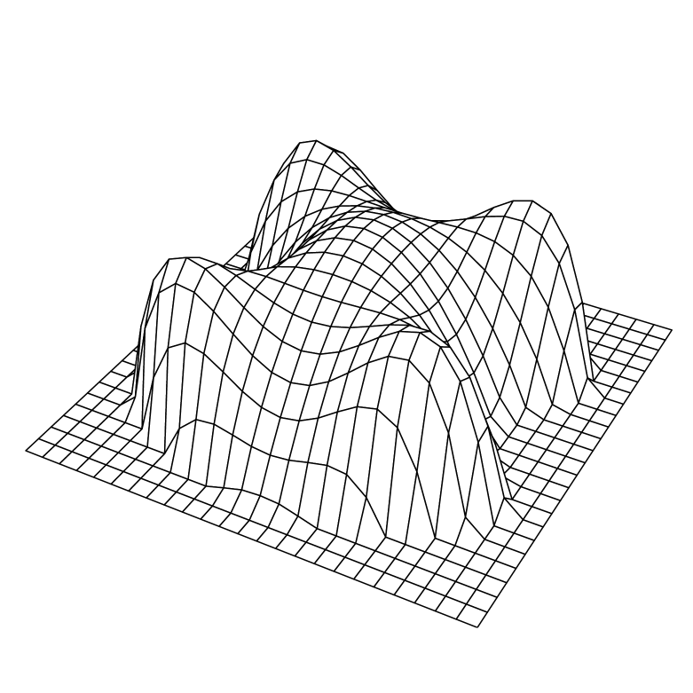
The potential $V(x,y)$ for a particular choice of parameters is shown in Fig 1(a).

FIG. 1.: (a) Illustrative plot of $V(x,y)$ with $\alpha=\beta=2$, $\gamma=4$, $\delta=\epsilon=1/5$. (b) Contours of zero force.

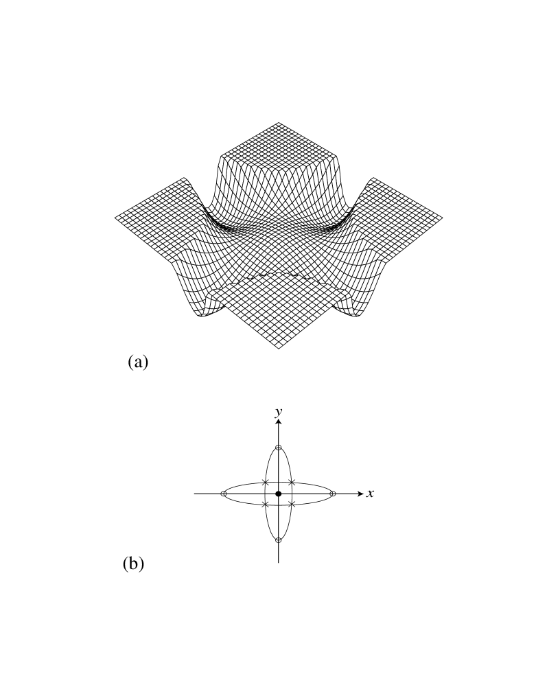
Before discussing the dynamics of the system, we have to identify the extrema of the potential. These are given by the intersection of the two sets of curves $\partial V/\partial x=0$ and $\partial V/\partial y=0\,$ or, explicitly, by the intersection of $\{x=0,\delta x^{2}+\gamma y^{2}=\alpha\}$ and $\{y=0,\gamma x^{2}+\epsilon y^{2}=\beta\}$. These two ellipses, along with the $x$ and $y$-axes, are shown in Fig 1(b). By comparing Figs 1(a) and Fig 1(b) we see that there is (i) a maximum at the origin (denoted by a filled circle), (ii) four minima at the intersection of the ellipses and the axes (denoted by open circles), and (iii) four saddle points at the intersection of the two ellipses (denoted by crosses). The precise positions of these extrema are:

$${\rm Minima}:\ \ (x,y) = \left(\pm\left(\frac{\alpha}{\delta}\right)^{1/2},\,0\right)\ \ ;\ \ (x,y)=\left(0,\ \pm\left(\frac{\beta}{\epsilon}\right)^{1/2}\right)\,.$$ (7)

$${\rm Saddles}:\ \ (x,y) = \frac{1}{\sqrt{\gamma^{2}-\delta\epsilon}}\left(\pm\sqrt{\beta\gamma-\alpha\epsilon},\ \pm\sqrt{\alpha\gamma-\beta\delta}\right)\,.$$ (9)

In fact, there are some conditions which need to be imposed on the parameters of the model if saddle points are to exist. These are that $\alpha\gamma-\beta\delta$, $\beta\gamma-\alpha\epsilon$ and $\gamma^{2}-\delta\epsilon$ should all have the same sign. Since we will normally assume that the stability parameters, $\delta$ and $\epsilon$, which ensure that the potential is bounded below, are small, we will take $\beta\gamma>\alpha\epsilon$ and $\alpha\gamma>\beta\delta$, which implies that $\gamma^{2}>\delta\epsilon$.

The dynamics given by (2), (5) and (6) is equivalent to an overdamped particle moving on the potential surface shown in Fig 1(a) and which is also acted upon by white noise. In a typical realization, the particle will begin at the maximum and perform a random walk which is in the vicinity of the origin at early times, but which eventually explores an ever larger region. Eventually, the particle gets far enough from the origin that the deterministic dynamics, specified by $V$, begins to have a significant impact and the particle accelerates down towards the saddles and the minima. In this paper our main concern is state selection: we are not concerned with the approach the particle makes to a particular minimum, since by this stage this minimum will almost certainly be the selected state. For this not to be so, the particle would have to hop over a barrier — an extraordinarily rare event. In fact, as is clear from Fig 1(a), as soon as the particle has passed the $x$ or $y$ coordinate of one of the saddle points, it has effectively chosen the final state and its subsequent motion is of little interest to us. We therefore arrive at the conclusion that the saddle points are the major factor influencing state selection and by comparison the minima are of little consequence. This can be made more transparent if we imagine that $\delta$ and $\epsilon$ are very small, so that the minima (7) are now at very large values of $x$ and $y$. By contrast, the positions of the saddles have changed much less: in the limit where $\delta$ and $\epsilon$ go to zero their $x$ and $y$ coordinates tend to the finite values $\sqrt{\beta/\gamma}$ and $\sqrt{\alpha/\gamma}$, whereas the minima tend to infinity. The topography now consists of long valleys, leading from the head of the valley between two saddles, all the way down to a minima at the end of the valley. As soon as the particle enters the valley it is extremely unlikely to escape over the sides, and so extremely unlikely it will do anything else but move to the minima at the end of that particular valley. This makes it very clear that it is the saddles, and not the minima, that we should focus on if we wish to understand state selection.

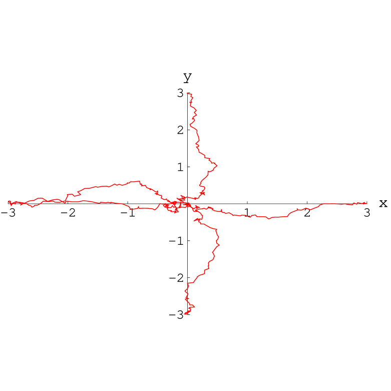
These ideas are well illustrated by plotting out a few Monte Carlo trajectories. Such simulations are extremely simple to carry out, and later we will compare our analytic expression for the probability of a particular state being selected with the proportion of runs which ended up in that state. For the moment, however, we are interested in the nature of individual trajectories. The five which are shown in Fig 2 are typical: the particle carries out Brownian motion about the origin, to a greater or lesser extent, and then selects a particular valley. Even after state selection, there may still be large deviations, but eventually the particle settles down near to the axis along which the valley runs.

FIG. 2.: Typical trajectories for the full potential $V(x,y)$ with $\alpha=\beta=\gamma=1$, $\delta=\epsilon=0.1$, and with noise strength $D=0.01$.

III The Reduced Potential

We have seen in the last section that the essential features of state selection become much clearer in the limit $\delta,\epsilon\rightarrow 0$, when the saddle points are completely separated from the minima, which have moved off to infinity. For the rest of the paper we work in this limit in order to illustrate our method in the simplest possible way. We will call the problem defined in Sec. II when the limit is taken, the reduced problem. The reduced potential is then defined to be

$$V_{R}(x,y)=-\frac{\alpha}{2}x^{2}-\frac{\beta}{2}y^{2}+\frac{\gamma}{2}x^{2}y^{2}\,.$$ (10)

A plot of $V_{R}$ looks very similar to the plot of the full potential $V$ in Fig 1(a), since this figure emphasizes the little-changed central features of the potential. The main difference is that whereas in $V$ the valley floors start to ascend again at large $|x|$ and $|y|$, in $V_{R}$ they keep descending. However, as was made clear in Sec II, this behavior is of no interest to us, and the fact that $V$ and $V_{R}$ differ in this way is immaterial.

From (10), we see that $V_{R}$ has only two types of extrema: (i) a maximum at the origin, and (ii) four saddle points at $(x,y)=(\pm X_{\rm min},\pm Y_{\rm min})$ where

$$X_{\rm min}=\sqrt{\frac{\beta}{\gamma}}\ \ ,\ \ Y_{\rm min}=\sqrt{\frac{\alpha}{\gamma}}\,.$$ (11)

The reason for the subscript “min” is that the values given by (11) are the smallest values of $|x|$ and $|y|$ at which we can assume that state selection has taken place. A simple stability analysis near these saddles shows that the stable and unstable directions are at an angle of $\pi/4$ to the axes. For example, in the positive quadrant, if the particle approaches the saddle along the line of steepest descent $y=x$, it will have a tendency to move down the slopes which are to the right and left, rather than carry on through the saddle and straight up the incline ahead.

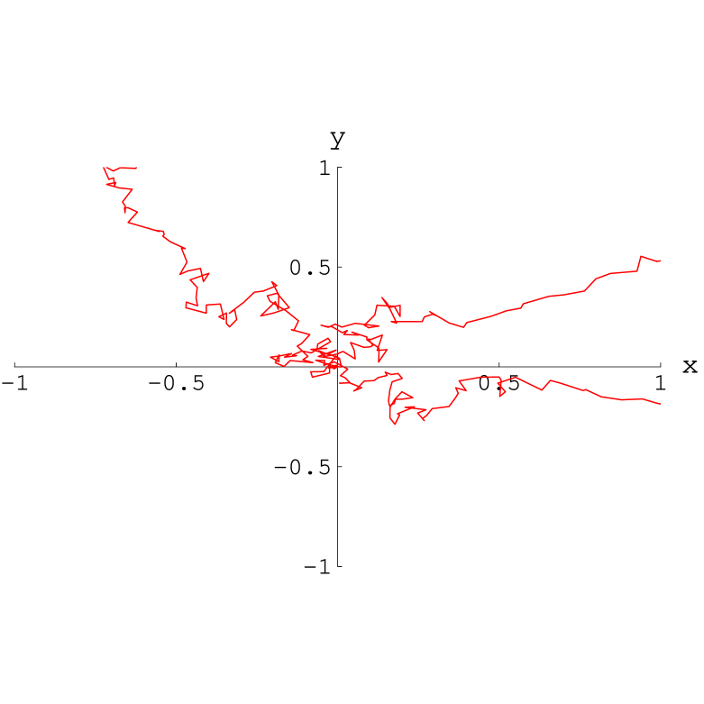
Just as the plot of $V_{R}$ is similar to that of $V$ if we cut it off near to the head of the valleys, so the Monte Carlo simulations are similar in both cases if we do not follow the trajectories too deeply into the valleys. In Fig. 3, the range of $x$ and $y$ used to display the trajectories are smaller than those in Fig. 2, so that the central region is emphasized. This makes the initial Brownian dynamics seem more obvious, but in reality the nature of the trajectories before and during state selection are essentially identical to those of the full problem shown in Fig. 2.

FIG. 3.: Typical trajectories for the reduced potential $V_{R}(x,y)$ with $\alpha=\beta=\gamma=1$, and with noise strength $D=0.01$.

In the next section, we will develop a calculational scheme, based on the path-integral formulation of the stochastic process, to determine the probabilities of entering the $x$- or $y$-valleys as a function of the model parameters $\alpha,\beta,\gamma$ and $D$. However, one might feel that such a sophisticated theory is not necessary: it should be possible to obtain a satisfactory theory by constructing an approximation based on the picture we have built up in this and the previous section. We will therefore end this section by constructing an example of such a theory and show that it is unsatisfactory for a variety of reasons.

A simple theory of state selection might have the following ingredients:

• In the initial period the noise and linear growth of the modes dominate. Therefore, neglect the non-linear interaction between the modes (i.e. set $\gamma=0$).

• State selection will be specified in the following way. Define four sectors in the $xy$-plane by drawing lines through the origin and the saddle points. The particle will select the state corresponding to a particular sector if it is in that sector for $x\approx X_{\rm min}$ and $y\approx Y_{\rm min}$.

A calculation based on these two assumptions is given in Appendix A. Even within the framework that these provide, there turn out to be many possible variants, each giving slightly different results. Leaving this aside for the moment, it is shown in Appendix A that in one of the simplest schemes along these lines, the probability of ending up in an $x$-valley is (see Eqn. (A16))

$$N_{x}=\frac{1}{1+\hat{D}^{\rho}}\,,$$ (12)

where

$$\hat{D}\equiv\frac{\gamma D}{\alpha\beta}\ \ {\rm and}\ \ \rho=\frac{(\alpha-\beta)}{\alpha}\,.$$ (13)

This has the correct qualitative behavior: when $\alpha=\beta$, that is, $\rho=0$, $N_{x}=1/2$. As $\rho$ increases, $N_{x}$ increases towards unity. A more careful calculation gives (Eqn. (A17))

$$N_{x}=\frac{2}{\pi}\tan^{-1}\hat{D}^{-\rho}\,.$$ (14)

which again has the correct qualitative features.

We now compare these two formulas with the results of Monte Carlo simulations. We took $\beta,\gamma$ and $D$ to be fixed in the simulations, at values $1.0,1.0$ and $0.01$ respectively, and varied $\alpha$ from $1.0$ to $3.0$ in steps of 0.2. For each value of $\alpha$ we performed a large number of runs where the particle started at the origin and ended up in one or other of the valleys (for more details see Sec. VI). We then simply counted the number of times that the particle ended up in a particular valley and expressed this as a fraction of the total number of runs made. The results are shown in Fig. 4.

FIG. 4.: Probability of flowing into an $x$-valley as a function of $\alpha$, with $\beta=1$, $\gamma=1$ and $D=0.01$. The dots show simulation results, the full curve is the result (12) and the dashed curve is result (14).

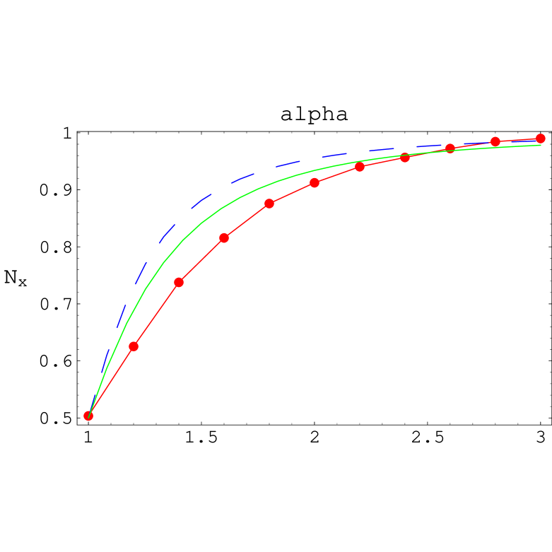
It is clear that the results of the naive approach based on assumptions 1 and 2 above, worked out in Appendix A and given by (12) and (14) are not quantitatively correct. They mainly overestimate the probability of the particle ending up in the $x$-valley. In addition, Eqn. (14), which represents a more refined calculation, actually compares less favorably with the simulation results, than does (12). This clearly points to the unsatisfactory nature of this simple-minded scheme, as one would expect the more refined calculation to compare more favorably with the simulation results.

We do not wish to pursue techniques based on this approach further in this paper. It was included specifically to show that there is a delicate interplay between the non-linearity and the noise in (3) and (4) and any attempt to incorporate one or the other of these using an unsystematic approximation scheme, as above, is likely to give disappointing results. We do not rule out being able to construct a particular scheme of this type which will give reasonable results: there are enough possible variants that it may be possible to interpolate between these by introducing free parameters which can then be fitted to the Monte Carlo data. However, such an ad hoc scheme is unnecessary, since we will show in the remainder of the paper that a systematic approach exists which gives simple formulas which are in good agreement with the Monte Carlo data. The method is based on the use of optimal paths, and so we begin with a brief review of the path-integral formulation of Langevin dynamics.

IV Optimal paths

In this section we review the formulation of stochastic differential equations, such as (2), as functional integrals and obtain the dominant contribution to the conditional probability we wish to determine in the limit where the noise strength tends to zero.

The conditional probability that the system is in the state $(x_{f},y_{f})$ at time $T$, given it was initially in the state $(0,0)$ at $t=0$ is

$$P(x_{f},y_{f},T|0,0,0)=\left\langle\delta\left(x_{f}-x(T)\right)\delta\left(y_{f}-y(T)\right)\right\rangle_{\rm IC}\,,$$ (15)

where IC denotes the initial condition $x(0)=0$, $y(0)=0$ on the stochastic process and $x(T)$ and $y(T)$ are solutions of (3) and (4). The average in (15) is over Gaussian white noises $\eta_{x}(t)$ and $\eta_{y}(t)$ with zero mean and correlation function given by (5). In terms of functional integrals (15) equals

$${\cal C}\int_{\rm IC}D\eta_{x}D\eta_{y}\,\delta\left(x_{f}-x_{\eta}(T)\right)\delta\left(y_{f}-y_{\eta}(T)\right)\,\exp\left\{-\frac{1}{4D}\int^{T}_{0}dt\left[\eta^{2}_{x}(t)+\eta^{2}_{y}(t)\right]\right\}\,,$$ (16)

where ${\cal C}$ is a normalization constant and the subscript $\eta$ on $x(T)$ and $y(T)$ is to emphasize that they depend on $\eta(T)$ through (3) and (4). Using these equations to perform a functional change of variable from $(\eta_{x},\eta_{y})$ to $(x,y)$ yields

$${\cal C}\int_{\rm IC}DxDy\,J\,\delta\left(x_{f}-x(T)\right)\delta\left(y_{f}-y(T)\right)\exp\left\{-\frac{1}{4D}\int^{T}_{0}dt\left[\left(\dot{x}+\frac{\partial V}{\partial x}\right)^{2}+\left(\dot{y}+\frac{\partial V}{\partial y}\right)^{2}\right]\right\}\,,$$ (17)

where $J$ is the Jacobian of the transformation. Expressed as a path-integral

$$P(\vec{r}_{f},T|\vec{0},0)={\cal C}\int^{\vec{r}(T)=\vec{r}_{f}}_{\vec{r}(0)=\vec{0}}D\vec{r}\,J[\vec{r}]\,\exp\left\{-S[\vec{r}]/D\right\}\,,$$ (18)

where $\vec{r}=(x,y)$. The action $S[\vec{r}]$ and the Jacobian $J[\vec{r}]$ are functionals which are given by

$$S[x,y]=\frac{1}{4}\int^{T}_{0}dt\,\left[\left(\dot{x}+\frac{\partial V}{\partial x}\right)^{2}+\left(\dot{y}+\frac{\partial V}{\partial y}\right)^{2}\right]\,,$$ (19)

and[26]

$$J[x,y]={\rm Det}\left[\frac{\delta\vec{\eta}}{\delta\vec{r}}\right]\propto\exp\left\{\frac{1}{2}\int^{T}_{0}dt\left[\frac{\partial^{2}V}{\partial x^{2}}+\frac{\partial^{2}V}{\partial y^{2}}\right]\right\}\,.$$ (20)

For $D\rightarrow 0$, the path-integral (18) is dominated by solutions of the Euler-Lagrange equations $\delta S/\delta\vec{r}(t)=0$, which satisfy the boundary conditions $\vec{r}(0)=0$ and $\vec{r}(T)=\vec{r}_{f}$. Let the solution of least action be denoted by $\vec{r}_{c}(t)$. Then writing $\vec{r}(t)=\vec{r}_{c}(t)+\delta\vec{r}(t)$, we have

$$P(\vec{r}_{f},T|\vec{0},0)={\cal C}\,\exp\left\{-S(\vec{r}_{c})/D\right\}\,\int D\delta\vec{r}\,J[\vec{r}_{c}+\delta\vec{r}]$$

$$\times\exp\left\{-\frac{1}{D}\int^{T}_{0}dt^{\prime}\int^{T}_{0}dt^{\prime\prime}\delta\vec{r}(t^{\prime})\left[\frac{1}{2}\left.\frac{\delta^{2}S}{\delta\vec{r}(t^{\prime})\delta\vec{r}(t^{\prime\prime})}\right|_{\vec{r}=\vec{r}_{c}}\right]\delta\vec{r}(t^{\prime\prime})+O(\delta\vec{r})^{3}\right\}\,.$$ (21)

Scaling $\delta\vec{r}$ by $D^{1/2}$ and performing the Gaussian functional integral yields

$$P(\vec{r}_{f},T|\vec{0},0)={\cal C^{\prime}}\,\exp\left\{-S(\vec{r}_{c})/D\right\}\,J(\vec{r}_{c})\,{\rm Det}\left[\left.\frac{\delta^{2}S}{\delta\vec{r}(t^{\prime})\delta\vec{r}(t^{\prime\prime})}\right|_{\vec{r}=\vec{r}_{c}}\right]^{-1/2}\left[1+O(D)\right]\,.$$ (22)

The new overall constant, ${\cal C^{\prime}}$, is immaterial since, as we have seen in Sec. III, we are interested only in the probability of ending up in the $x$-valley or $y$-valley, and we normalize these probabilities according to $N_{x}+N_{y}=1$. We will therefore omit the overall constant from now on.

While all the derivations in this section have been carried out for potential systems with two degrees of freedom, it should be clear that they generalize in an obvious way to systems of more than two degrees of freedom and those where no potential exists[26]. We may summarize the result of performing the functional steepest descent on (18) to next-to-leading order by

$$P(\vec{r}_{f},T|\vec{0},0)=P^{(1)}(\vec{r}_{f},T)\exp\left\{-P^{(0)}(\vec{r}_{f},T)/D\right\}\,\left[1+O(D)\right]\,,$$ (23)

where the leading order contribution, $P^{(0)}$, is just the action of the optimal path $\vec{r}_{c}(t)$ and the next-to-leading order contribution is

$$P^{(1)}(\vec{r}_{f},T)=J(\vec{r}_{c})\,\left({\rm Det}L(\vec{r}_{c})\right)^{-1/2}\,.$$ (24)

Here $L$ is the matrix formed from the second order functional derivative of the action functional evaluated at the optimal path:

$$L(\vec{r}_{c})=\left.\frac{\delta^{2}S}{\delta\vec{r}(t^{\prime})\delta\vec{r}(t^{\prime\prime})}\right|_{\vec{r}=\vec{r}_{c}}\,.$$ (25)

The result (23) is the starting point for our method: if we can determine the functions $P^{(0)}$ and $P^{(1)}$, then we will have a form for the conditional probability valid when the noise is weak. This in turn will enable us to obtain a formula for the probability that either the $x$-valley or $y$-valley is selected, as a function of $\alpha,\beta,\gamma$ and $D$. We shall devote the rest of this section to the determination of $P^{(0)}$ and leave the calculation of $P^{(1)}$ to the next section.

The case of interest to us in this paper is when $V$ is the reduced potential (10). The Euler-Lagrange equations for this problem are

$$\ddot{x} = x\left(\alpha-\gamma y^{2}\right)^{2}-2\gamma xy^{2}\left(\beta-\gamma x^{2}\right)\ \ {\rm and}$$ (26)

$$\ddot{y} = y\left(\beta-\gamma x^{2}\right)^{2}-2\gamma yx^{2}\left(\alpha-\gamma y^{2}\right)\,.$$ (27)

It is important to realize that there are two distinct dynamics associated with the problem under consideration. The first is the stochastic dynamics given by (2) with the potential (10). This was our starting point, the basis of the intuitive discussion of the dynamics given in Secs. II and III, and the dynamics of the Monte Carlo simulation. The second dynamics is the deterministic dynamics, given by (26) and (27), which describes the $D\rightarrow 0$ limit of the stochastic dynamics. They are quite different and it is important not to carry over intuition from one to the other without careful consideration. From (19),

$$S[\vec{r}]=\frac{1}{2}\int^{T}_{0}dt\left[\frac{1}{2}\dot{\vec{r}}^{2}-U(\vec{r})\right]+\frac{1}{2}\int^{T}_{0}dt\frac{dV}{dt}\,,$$ (28)

where

$$U(\vec{r})=-\frac{1}{2}\left(\frac{\partial V}{\partial x}\right)^{2}-\frac{1}{2}\left(\frac{\partial V}{\partial y}\right)^{2}\,.$$ (29)

Since the last term in (28) is a constant, and consequently gives zero variation, the Euler-Lagrange equations (26) and (27) correspond to classical mechanics in the potential

$$U_{R}(x,y)=-\frac{1}{2}x^{2}(\alpha-\gamma y^{2})^{2}-\frac{1}{2}y^{2}(\beta-\gamma x^{2})^{2}\,.$$ (30)

When considering the optimal paths such as $\vec{r}_{c}(t)$, it is the potential $U_{R}$, and not $V_{R}$, that is relevant. A plot of $U_{R}(x,y)$ is shown in Fig. 5.

FIG. 5.: Illustrative plot of the reduced potential $U_{R}(x,y)$ with $\alpha=2$, $\beta=\gamma=1$.

We will, for concreteness, focus on paths which end in the positive $x$-valley; paths which end in the other valleys are treated in exactly the same way. The boundary conditions on these paths are $x(0)=y(0)=0$, $x(T)=x_{f}$ and $y(T)=y_{f}$, with $y_{f}\ll x_{f}$. We therefore simplify (26) and (27) by keeping only terms which are linear in $y$, to obtain to lowest order,

$$\ddot{x} = \alpha^{2}x\ \ {\rm and}$$ (31)

$$\ddot{y} = \left[\beta^{2}-2(\alpha+\beta)\gamma x^{2}+\gamma^{2}x^{4}\right]\,y\,.$$ (32)

In our earlier treatment of this problem[1], we restricted attention to end-points lying on the $x$-axis: $x_{f}=X$ and $y_{f}=0$ (and correspondingly $y_{f}=Y$ and $x_{f}=0$ for paths ending in the positive $y$-valley) arguing that the relative contributions coming from paths ending on the axes should be approximately equal to the relative contributions coming from the paths ending anywhere in the valleys. In fact, as shown in Ref. [1], this turns out to be an excellent approximation, but it has the deficiency that $X$ is not determined. In this paper, we go beyond this approximation, which allows us to explore its validity, but also, as we will see, the precise value of $X$ within this improved treatment does not enter; the result is independent of $X$, provided that $X$ is large enough. The quantity $y_{f}$ has a different character to $X$: it will be integrated over at a later stage, when the probability flux through the valley is determined.

The solution of (31) which satisfies the boundary conditions $x(0)=0$ and $x(T)=X$ is exactly the same as in Ref. [1], namely,

$$x_{c}(t)=X\frac{\sinh\alpha t}{\sinh\alpha T}\,.$$ (33)

The solution of (32) which satisfies the boundary conditions $y(0)=0$ and $y(T)=y_{f}$ (we reserve the notation $Y$ for the final $y$ value for the end-point of paths going along the $y$-valleys) is discussed in Appendix B. There it is shown that an excellent approximation to the solution of this equation (indistinguishable from the numerical solution) can be found by first solving the equation for small $t$ and then for large $t$, and matching the two at some intermediate matching time $t_{m}$. Comparison with the numerical solution shows that the approximation remains good for a wide range of values of $t_{m}$ from about $0.1T$ to $0.6T$ or $0.7T$. In order to be able to obtain a simple form for the solution, we have assumed that $T$ is large, in the sense that $e^{-\alpha T}\ll 1$ and $e^{-\beta T}\ll 1$. Using (B3) and (B7), we can write the explicit analytic from as

$$y_{c}(t)=\left\{\begin{array}[]{ll}\ \ \ \ \ \ \ 2y_{f}\,e^{-\beta T}\,e^{\gamma X^{2}/2\alpha}\,\sinh\beta t,&\mbox{\ $0\leq t\leq t_{m}$}\\ y_{f}\,e^{-\beta(T-t)}\exp\left[\frac{\gamma X^{2}}{2\alpha}\left\{1-e^{-2\alpha(T-t)}\right\}\right],&\mbox{\ $t_{m}\leq t\leq T$\, .}\end{array}\right.$$ (34)

For self-consistency we need to check that $y_{c}(t)$ given by (34) is small, compared with $x_{c}(t)$, if we are to justify the linearization procedure which led to (31) and (32). From (34) it is straightforward to check that $y_{c}(t)$ has a maximum at $t=t^{\prime}$, where $t^{\prime}=T$, if $X<X_{\rm min}$ and $T-t^{\prime}=\alpha^{-1}\,\ln(X/X_{\rm min})$, if $X>X_{\rm min}$. As discussed in Sec. III, $X_{\rm min}$ is the minimum value of $x$ at which state selection can be said to have been completed, and therefore we ask that $X\geq X_{\rm min}$. The maximum value of $y_{c}(t)$,

$$y_{c}(t^{\prime})=y_{f}\,\left(\frac{X}{X_{\rm min}}\right)^{-\beta/\alpha}\,\exp\left\{\frac{\gamma}{2\alpha}\,\left(X^{2}-X^{2}_{\rm min}\right)\right\}\,,$$ (35)

increases rapidly with $X$ and is already extremely large when $X\sim 5X_{\rm min}$. It might therefore be tempting to argue that we need to take $X$ to be much less than this value if the linearization procedure is to be valid. Since (35) has its least value when $X=X_{\rm min}$, this approximation would seem to be best for this choice of $X$, and in fact this was the choice made in our earlier work[1].

In fact, there are a variety of reasons why choosing $X$ to be $X_{\rm min}$ is not suitable. First, the argument above, namely that if $X$ is too large then the linearization procedure is invalid, is in fact incorrect. We will find that the width of the distribution is so narrow in the $y$ direction that the range of integration for $y_{f}$ need only be tiny — in fact only going out to values of $y_{f}$ such that $y_{f}^{2}\exp\left\{\gamma X^{2}/\alpha\right\}\sim 1$. From (35) we see that under these conditions $y_{c}(t)$ is indeed small. We will come back to this point again in Secs. VI and VII.

The second reason is in fact more profound. Intuitively, we expect that for large enough values of $X$ the probability flux through a given valley should be independent of $X$. This is due to the fact that in the regime of weak noise, once state selection has occurred there is no flux leakage out of a valley. This implies that we should not have to make any choice for $X$ because our results should be independent of $X$ as long as $X$ is large enough. In fact, this is precisely what we find, namely that the probability flux through the $x$-valley tends to an asymptotic value as $X$ tends to infinity. The remarkable cancellations that occur to produce an $X$ independent flux is a good indicator of the correctness of our calculational scheme. Again, we will come back to this point in Secs. VI and VII.

Finally, throughout our calculation we use the approximation that $T$ is large in the sense that $e^{-\alpha T}\ll 1$ and $e^{-\beta T}\ll 1$. This is apparently a problem, since we need the form of the distribution for all $T$ in order to perform the time integral of the probability flux in the calculation of the total flux through the valley. The way out of this impasse is to take $X$ sufficiently large that the probability current is essentially zero at small times, and only starts making appreciable contributions to the $T$ integral when $T$ is such that $e^{-\alpha T}\ll 1$ and $e^{-\beta T}\ll 1$. It is not clear how large $X$ will have to be, but as discussed above, the probability flux through the $x$-valley tends to an asymptotic value as $X$ grows, so we are assured of always finding a value of $X$ for which the approximation that $T$ is large is valid.

At first sight, the large $T$ approximation might appear to be problematic because it ignores the shorter state selection time scales $\alpha^{-1}$ and $\beta^{-1}$. However, this is not the case. The reason is that the integrals over time that are performed in the calculation of the action and Jacobian prefactor include these earlier times. In other words, the entire classical path, in particular the spatial region near the origin, is included in the calculation.

After these rather technical asides, it is worthwhile summarizing what we have deduced about the equation for the optimal path which leaves $(0,0)$ at $t=0$ and arrives at $(X,y_{f})$ at time $t=T$. It is given by (33) and (34) under the assumptions that (i) $T$ is such that $e^{-\alpha T}\ll 1$ and $e^{-\beta T}\ll 1$, (ii) $X$ is larger than a few $X_{\rm min}$, and (iii) $t_{m}$ and $(T-t_{m})$ are large (we will later find that we require that $e^{-2\alpha t_{m}}\ll 1,e^{-2\beta t_{m}}\ll 1,e^{-2\alpha(T-t_{m})}\ll 1$ and $e^{-2\beta(T-t_{m})}\ll 1$).

We are now in a position to calculate the leading order contribution, $P_{0}(X,y_{f},T)$, to the conditional probability distribution (23), by finding the action of the optimal path given by (33) and (34). We begin by noting that, from (28), the classical paths are solutions of $\ddot{x}=-\partial U/\partial x$ and $\ddot{y}=-\partial U/\partial y$. Multiplying the first equation by $\dot{x}$, the second one by $\dot{y}$, adding them and integrating the result, gives $\frac{1}{2}(\dot{x}^{2}_{c}+\dot{y}^{2}_{c})+U=E$, a constant. Thus another form for the action of classical paths is

$$S_{c}=\frac{1}{2}\int^{T}_{0}dt\,\left[\dot{x}^{2}_{c}+\dot{y}^{2}_{c}\right]-\frac{1}{2}ET+\frac{1}{2}\left[V\right]^{T}_{0}\,.$$ (36)

Details of the calculation are given in Appendix B. From (B23) we find

$$S_{c}=\frac{\alpha X^{2}}{4}\,\left({\rm coth}\alpha T-1\right)+\frac{1}{2}\,y^{2}_{f}\,S_{y}\,,$$ (37)

where

$$S_{y}=\frac{1}{2\alpha}\,\left(\frac{\alpha}{\gamma X^{2}}\right)^{\beta/\alpha}\,\exp\left\{\frac{\gamma X^{2}}{\alpha}\right\}\,\int^{\gamma X^{2}/\alpha}_{0}dz\,z^{(\beta/\alpha)-1}\,e^{-z}\,(\beta-\alpha z)^{2}+\frac{1}{2}[\gamma X^{2}-\beta]\,.$$ (38)

The two terms in (37) have different characters: as remarked earlier, we will eventually integrate over $y_{f}$ to obtain the probability flux through the valley, but the first term will remain, giving a leading order contribution of $\exp{-(\alpha X^{2}/4D)({\rm coth}\alpha T-1)}$ to (23).

When performing similar calculations to find the escape rate from one metastable state to another, the leading order result $e^{-\Delta V/D}$ gives a reasonable estimate, and the need to go to next order and to calculate the prefactor only arises if increased accuracy is required. The situation is very different in the present case of the decay from an unstable state. As mentioned already, we expect that the main contribution to the probability flux through the valley will occur when $T\sim(2\alpha)^{-1}\,\ln(\alpha X^{2}/D)$. The conditional probability distribution (23) is peaked around a value of $T$ of this order because of a balance between the leading (classical) term and the prefactor (a fluctuational) term. For this reason, the calculation of the prefactor in this problem, unlike in escape problems, is vital if the essential structure of the state selection probabilities is to be captured. We therefore turn to the calculation of this quantity.

V Calculation of the prefactor

In this section we will calculate the next to leading order contribution in (23). From (24) we see that it consists of two distinct contributions: from the Jacobian $J[\vec{r}]$ evaluated at the optimal path, and from the fluctuations around the optimal path which give rise to the determinant of the second functional derivative of the action (25). We begin by evaluation of this determinant.

Starting from (28), and using the notation (25), we obtain

$$L(\vec{r}_{c})=\left[\matrix{&&\vrule height=17.0pt,depth=5.0pt&&&&\cr&-\frac{d^{2}}{dt^{2}}+\alpha^{2}&\vrule height=17.0pt,depth=5.0pt&&-4\gamma x_{c}y_{c}\left[\alpha+\beta-\gamma x_{c}^{2}\right]&&\cr\vskip-3.0pt\cr&&\vrule height=17.0pt,depth=5.0pt&&&&\cr\hrule\cr&&\vrule height=17.0pt,depth=5.0pt&&&&\cr\vskip-3.0pt\cr&-4\gamma x_{c}y_{c}\left[\alpha+\beta-\gamma x_{c}^{2}\right]&\vrule height=17.0pt,depth=5.0pt&&-\frac{d^{2}}{dt^{2}}+\left(\beta-\gamma x_{c}^{2}\right)^{2}-2\alpha\gamma x_{c}^{2}&&\cr\vskip-3.0pt\cr&&\vrule height=17.0pt,depth=5.0pt&&&&\cr}\right]\,,$$ (39)

where, in line with our previous assumption, we have neglected terms which are $O(y_{c}^{2})$ down on the terms shown in (39). We have omitted any time dependence in (39) for the sake of clarity, but it should be remembered that the classical solutions $x_{c}$ and $y_{c}$ are functions of $t$ and the matrix is multiplied by an overall factor of $\delta(t-t^{\prime})$. The diagonal entries are as in the $y_{c}=0$ case[1] — only the off-diagonal entries are different. However, it is easy enough to see that the eigenvalues of (39) are even in $y_{c}$, and since the matrix with $y_{c}=0$ has no zero eigenvalues, the off-diagonal entries only provide $O(y^{2}_{c})$ corrections to the eigenvalues of the matrix with $y_{c}=0$. Therefore neglecting these terms as before, we conclude that within the approximation we have adopted in this paper, we may set the off-diagonal entries in (39) to zero. From (25) and (39) we now find

$${\rm Det}L(\vec{r}_{c})={\rm Det}L_{x}\,{\rm Det}L_{y}\,,$$ (40)

where $L_{x}$ and $L_{y}$ represent fluctuations in $x$ and $y$ respectively:

$$L_{x} = -\frac{d^{2}}{dt^{2}}+\alpha^{2}\,,$$ (41)

$$L_{y} = -\frac{d^{2}}{dt^{2}}+\left(\beta-\gamma x^{2}_{c}\right)^{2}-2\alpha\gamma x^{2}_{c}\,.$$ (42)

To evaluate the determinants of the operators (41) and (42) we make use of a well-known formula for such determinants[28]. Let $L$ be an operator of the type $-d^{2}/dt^{2}+\phi(t)$ and suppose that the eigenfunctions of $L$ are required to vanish at the boundaries at $t=0$ and $t=T$, as in the case of interest to us here. Now let $h_{1}(t)$ and $h_{2}(t)$ be two independent solutions of the homogeneous equation $Lh=0$. Then

$${\rm Det}L\propto\frac{h_{1}(0)h_{2}(T)-h_{2}(0)h_{1}(T)}{h_{1}(0)\dot{h}_{2}(0)-h_{2}(0)\dot{h}_{1}(0)}\,.$$ (43)

The constant of proportionality in (43) may be omitted for the same reason the overall constant was omitted in (22): the probability of ending up in the positive $x$-valley will be normalized by the sum of the probabilities of ending up in the $x$- and $y$-valleys. Furthermore, if $h_{2}$ is the solution which vanishes at $t=0$, then the formula for ${\rm Det}L$ involves only this solution:

$${\rm Det}L=\frac{h_{2}(T)}{\dot{h}_{2}(0)}\,.$$ (44)

The solution of $L_{x}h=0$ which satisfies $h(0)=0$ is $h_{2}(t)=F\sinh\alpha t$, where $F$ is a constant. Therefore

$${\rm Det}L_{x}=\frac{\sinh\alpha T}{\alpha}\,.$$ (45)

To find ${\rm Det}L_{y}$ we need only note that the solutions of the homogeneous equation $L_{y}h=0$ are also the solutions of the classical equation (32). But the solution which vanishes at $t=0$ has already been found in Appendix B: it is given by (B3) and (B7),

$$h_{2}(t)=\left\{\begin{array}[]{ll}\ \ \ \ \ \ \ G\sinh\beta t,&\mbox{\ $0\leq t\leq t_{m}$}\\ \frac{G}{2}\,e^{\beta t}\exp\left[-\frac{\gamma X^{2}}{2\alpha}\,e^{-2\alpha(T-t)}\right],&\mbox{\ $t_{m}\leq t\leq T$\, ,}\end{array}\right.$$ (46)

where $G$ is a constant. Since $\dot{h}_{2}(0)=\beta G$, use of (44) yields,

$${\rm Det}L_{y}=\frac{1}{2\beta}\,e^{\beta T}\,\exp\left\{-\frac{\gamma X^{2}}{2\alpha}\right\}\,.$$ (47)

It only remains to calculate the Jacobian at the optimal path. From (20) this is given by

$$J(\vec{r}_{c})=\exp\left\{\frac{1}{2}\int^{T}_{0}dt\left[\left(-\alpha+\gamma y^{2}_{c}(t)\right)+\left(-\beta+\gamma x^{2}_{c}(t)\right)\right]\right\}\,.$$ (48)

Neglecting the $O(y_{c}^{2})$ term as before, one finds that $J(\vec{r}_{c})=J_{x}J_{y}$ where

$$J_{x} = \exp\left\{-\frac{1}{2}\alpha T\right\}\,,$$ (49)

$$J_{y} = \exp\left\{-\frac{1}{2}\beta T+\frac{\gamma X^{2}}{4\alpha}\,\left[\frac{\sinh 2\alpha T-2\alpha T}{2\sinh^{2}\alpha T}\right]\right\}$$ (50)

$$\approx \exp\left\{-\frac{1}{2}\beta T+\frac{\gamma X^{2}}{4\alpha}\right\}\,,$$ (51)

since we are assuming that $e^{-\alpha T}\ll 1$. Since both the determinants and the Jacobians factorize into contributions associated with the $x$ coordinate and contributions associated with the $y$ coordinate, we may summarize the results of this section so far as

$$\frac{J_{x}}{\sqrt{{\rm Det}L_{x}}} = (2\alpha)^{1/2}\,e^{-\alpha T}\,,$$ (52)

$$\frac{J_{y}}{\sqrt{{\rm Det}L_{y}}} = (2\beta)^{1/2}\,e^{-\beta T}\,\exp\left\{\frac{\gamma X^{2}}{2\alpha}\right\}\,.$$ (53)

It is straightforward to check that these results agree with those of Ref. [1] under the assumptions that $e^{-\alpha T}\ll 1$ and $e^{-\beta T}\ll 1$. While neglecting corrections to the leading behavior of the prefactor which are of the type $e^{-2\alpha T}$ or $e^{-2\beta T}$ is in line with this large $T$ approximation, we will see later that the final integration over $T$ will also provide a posteriori justification for the neglect of these terms.

From (23), (37), (52) and (53), we can now write down the conditional probability for the system to be at $\vec{r}_{f}=(X,y_{f})$ at time $T$, given that it was at the origin at time $t=0$, as

$$P(\vec{r}_{f},T|\vec{0},0) = \left(4\alpha\beta\right)^{1/2}\,\exp\left\{-(\alpha+\beta)T+\frac{\gamma X^{2}}{2\alpha}\right\}$$ (54)

$$\times \exp\left\{-\frac{\alpha X^{2}}{4D}\,\left({\rm coth}\alpha T-1\right)\right\}\exp\left\{-\frac{y^{2}_{f}}{2D}\,S_{y}\right\}\,\left[1+O(D)\right]\,.$$ (55)

As we discussed in detail in Secs. II and III, when using the modified potential (10) the question is not what are the paths of least action from the origin to the minima of the potential, since those minima cease to exist when the limit $\delta,\epsilon\rightarrow 0$ is taken. Instead, the question is what is the relative flux through one valley compared to the other. To calculate the flux, it is not the conditional probability distribution (55) that we need to know, but the probability current $\vec{\cal J}=({\cal J}_{x},{\cal J}_{y})$. This current is related to the conditional probability distribution through the Fokker-Planck equation[29]

$$\frac{\partial P}{\partial t}+{\rm div}\vec{\cal J}=0\,,$$ (56)

where

$$\vec{\cal J}=-\left(\nabla V\right)P-D\nabla P\,.$$ (57)

In order to find $\vec{\cal J}$ from $P$ given by (55), we first note from (23) that

$$D\nabla P=-\left(\nabla P^{(0)}\right)P\left[1+O(D)\right]\,.$$ (58)

Therefore we only need to differentiate $V$ and $P^{(0)}$ with respect to $X$ and $y_{f}$ in order to find $\vec{\cal J}$. Carrying this out we obtain

$${\cal J}_{x} = \left(\frac{\alpha}{2}X\left[{\rm coth}(\alpha T)-1\right]+\alpha X-\gamma Xy_{f}^{2}\right)P$$ (59)

$${\cal J}_{y} = \left(S_{y}y_{f}+\beta y_{f}-\gamma y_{f}X^{2}\right)P\,.$$ (60)

In the next section we will calculate the flux through the positive $x$-valley. This will involve only the component of $\vec{\cal J}$ normal to the line $x=X$. Therefore, the $y$-component of the current, ${\cal J}_{y}$, will not contribute and need not be considered any further; the entire contribution to the flux will come from integrating ${\cal J}_{x}$, given by (59), over $y_{f}$. By virtue of the $y_{f}^{2}$ term in the exponential in (55) this will be a Gaussian integral. While we would naturally neglect the $O(y_{f}^{2})$ term in (59) in line with previous approximations in this section, we now see that it would in any case give a contribution of order $D$ once the $y_{f}$ integral is performed. This is a further justification for ignoring such terms. Finally, we have been neglecting $e^{-2\alpha T}$ type corrections in the prefactor, which means that we should replace ${\rm coth}\alpha T$ by $1$. These approximations lead to the result ${\cal J}_{x}=\alpha XP$ and so we find from (55)

$${\cal J}_{x}(X,y_{f},T) = 2\alpha(\alpha\beta)^{1/2}\,X\,\exp\left\{-(\alpha+\beta)T+\frac{\gamma X^{2}}{2\alpha}\right\}$$ (61)

$$\times \exp\left\{-\frac{\alpha X^{2}}{4D}\,\left({\rm coth}\alpha T-1\right)\right\}\exp\left\{-\frac{y^{2}_{f}}{2D}\,S_{y}\right\}\,\left[1+O(D)\right]\,.$$ (62)

This is the key result of this section. We need now only use it to calculate the total flux through the positive $x$-valley at $x=X$ and compare it with the analogous quantity through the positive $y$-valley. This will give us the relative probability of the $x$-mode being selected.

VI Results

The idea underlying the method we use to calculate the relative probability of one of the states being selected is most easily understood by first describing the analogous procedure used when carrying out Monte Carlo simulations. As was briefly alluded to in Sec. III, for each run the particle starts at the origin and subsequently follows the Langevin dynamics of the reduced problem until it reaches $x=\pm X$ in one of the $x$-valleys or $y=\pm Y$ in one of the $y$-valleys. We used $X=5X_{\rm min}$ and $Y=5Y_{\rm min}$ to be certain that state selection had occurred. At this point that particular run ceases. If the particle has ended up in a $y$-valley, for instance, 1 is added to the total number of runs which have selected the $y$-mode. Another run is initiated and the result of that is added to the totals. After a large number of runs the proportions selecting the $x$-mode and $y$-mode are used to calculate $N_{x}$ and $N_{y}$, the relative probabilities of these states being selected.

Let us focus on the runs ending up in the positive $x$-valley, exactly as we have been doing in the analytic treatment in Secs. IV and V. For each of these runs the final value of $y$ — called $y_{f}$ in the analytic treatment above — will vary. We would expect most of the runs to end near to the $x$-axis, with off-axis end-points becoming less and less common as we move away from the axis. This is reflected in the $y_{f}$ dependence of ${\cal J}_{x}$ given by (62). Just as in the Monte Carlo simulation, where we add up all contributions with differing final $y$-coordinate at $x=X$, so we need to integrate (62) over all $y_{f}$ at $x=X$. Similarly, just as in the Monte Carlo simulation, where we add up all of the contributions, no matter how long they took to get to the end-point, so in the analytic treatment we have to integrate over all $T$ to obtain the total flux. Therefore we need to calculate

$${\cal F}_{x}(X)=\int^{\infty}_{0}dT\,\int^{\infty}_{-\infty}dy_{f}\,{\cal J}_{x}(X,y_{f},T)\,,$$ (63)

in order to calculate the state selection probabilities.

While the above justification for (63) as the quantity which we need to calculate seems intuitively plausible, it is worthwhile formally proving this. We first need to specify what “ending up in the positive $x$-valley” means in terms of a mathematical expression. Since, in the limit $T\rightarrow\infty$, trajectories will have entered one of the four valleys, we define the probability that it has entered the positive $x$-valley as

$${\rm Prob}(+x{\rm-valley})=\lim_{T\rightarrow\infty}\,\int^{\infty}_{-\infty}dy_{f}\,\int^{\infty}_{X}dX\,P(X,y_{f},T|\vec{0},0)\,.$$ (64)

Here the positive $x$-valley is defined as the entire potential surface to the right of the line $x=X$. On the other hand from the continuity equation (56)

$$\lim_{T\rightarrow\infty}\,P(X,y_{f},T|\vec{0},0)-P(X,y_{f},0|\vec{0},0) = \int^{\infty}_{0}\frac{\partial}{\partial T}\,P(X,y_{f},T|\vec{0},0)\,dT$$ (65)

$$= -\int^{\infty}_{0}{\rm div}\vec{\cal J}\,dT\,.$$ (67)

Integrating (67) over the “volume” $\{x\geq X,-\infty<y_{f}<\infty\}$, using that fact that at $T=0$ the end-point is at the origin and making use of the divergence theorem, gives

$$\lim_{T\rightarrow\infty}\,\int^{\infty}_{-\infty}dy_{f}\,\int^{\infty}_{X}dX\,P(X,y_{f},T|\vec{0},0)=-\int^{\infty}_{0}dT\,\int_{S}\vec{\cal J}.d\vec{S}\,.$$ (68)

The “surface” integral on the right-hand side of (68) only gives a contribution at $x=X$, where $d\vec{S}$ is in the direction of the outward normal, i.e. in the negative $x$ direction. Thus $\vec{\cal J}.d\vec{S}=-{\cal J}_{x}dy_{f}$ and so the required probability (64) is equal to (63).

Substituting (62) into (63) and performing the $y_{f}$ integration yields

$${\cal F}_{x}(X) = 2\alpha(\alpha\beta)^{1/2}\,X\,\left(\frac{2\pi D}{S_{y}}\right)^{1/2}\,\exp\left\{\frac{\gamma X^{2}}{2\alpha}\right\}\,\int^{\infty}_{0}dT\,e^{-(\alpha+\beta)T}$$ (69)

$$\times \exp\left\{-\frac{\alpha X^{2}}{4D}\,\left({\rm coth}\alpha T-1\right)\right\}\left[1+O(D)\right]\,.$$ (70)

As remarked in Sec. V, any $O(y_{f}^{2})$ corrections in the prefactor give $O(D)$ corrections to (70), as do $O(y_{f}^{4})$ corrections to the action, which justifies their omission. The final integral over $y_{f}$ also provides justification for the linear approximation. An examination of ${\cal J}_{x}(X,y_{f},T)$ shows that this function is effectively non-zero only for small values of $|y_{f}|$, which get still smaller as $X$ increases, so that unless $|y_{f}|\lesssim\exp\left\{-\gamma X^{2}/2\alpha\right\}$, the flux is essentially zero. Thus either the conditional probability distribution or the conditional probability current resemble a thin wafer centered on the $x$-axis when plotted at fixed $T$. Moreover, this wafer gets very much thinner with increasing $X$. This means that the limits on the $y_{f}$ integral in (63) are effectively $\pm\exp\left\{-\gamma X^{2}/2\alpha\right\}$, which is tiny for large $X$. It is more instructive to change variables from $y_{f}$ to $y^{*}_{f}=y_{f}\,\exp\left\{\gamma X^{2}/2\alpha\right\}$, so that the integral now has the range $(-1,1)$. But, as discussed in Sec. IV, this means that (35) now reads

$$y_{c}(t^{\prime})=y^{*}_{f}\,\left(\frac{X}{X_{\rm min}}\right)^{-\beta/\alpha}\,\exp\left\{-\frac{\gamma X^{2}_{\rm min}}{2\alpha}\,\right\}\,,$$ (71)

which has a magnitude less than one for $-1<y^{*}_{f}<1$. Thus the linearization procedure is justified. In some sense, the variable $y^{*}_{f}$ is more appropriate in this problem than $y_{f}$ itself.

An examination of the integrand in (70) shows that is has a maximum when $T=T^{*}\equiv(2\alpha)^{-1}\ln(\alpha^{2}X^{2}/[(\alpha+\beta)D])$, which is slightly different to the value mentioned in Sec. IV. This is because that value came from the estimates of Sec. III and Appendix A, which used the value for the maximum which is found in the analogous one-dimensional stochastic process in $x(t)$. The more refined calculation we have been discussing here has an additional $e^{-\beta T}$ contribution coming from fluctuations in $y(t)$ and from $J_{y}$. It is the occurrence of this term in the integrand of (70) which changes the value at which the maximum occurs by this very slight amount. From (70) we can also check the conjecture made in Sec. IV, that if $X$ is greater than a few $X_{\rm min}$, then even the tails of the integrand will be at values of $T$ which are large enough for the approximations made in this paper to be valid. A numerical investigation of the integrand shows that it has typically already fallen by two orders of magnitude from its maximum value for $T$ satisfying $e^{-\alpha T},e^{-\beta T}\ll 1$, when $X$ is larger than a few $X_{\rm min}$.

To perform the integration in (70) we (i) replace $({\rm coth}\alpha T-1)$ by its large $T$ form, $2e^{-2\alpha T}$ (justified below), and (ii) change variables to $\xi=(\alpha X^{2}/2D)e^{-2\alpha T}$. Then the integral becomes

$$\frac{1}{2\alpha}\,\left(\frac{2D}{\alpha X^{2}}\right)^{(\alpha+\beta)/2\alpha}\,\int^{\Xi}_{0}d\xi\,\xi^{[(\alpha+\beta)/2\alpha]-1}\,e^{-\xi}\,,$$ (72)

where $\Xi=(\alpha X^{2})/2D$. The integral is an incomplete gamma function: it equals $\Gamma([\alpha+\beta]/2\alpha)$ plus exponentially small corrections in $D$ coming from the large, but finite, upper limit $\Xi$[27]. Neglecting these exponentially small terms we therefore obtain for the total flux through the positive $x$-valley at $X$

$${\cal F}_{x}(X)=(\alpha\beta)^{1/2}\,X\,\left(\frac{2\pi D}{S_{y}}\right)^{1/2}\,\exp\left\{\frac{\gamma X^{2}}{2\alpha}\right\}\,\left(\frac{2D}{\alpha X^{2}}\right)^{(\alpha+\beta)/2\alpha}\,\Gamma\left(\frac{\alpha+\beta}{2\alpha}\right)\left[1+O(D)\right]\,.$$ (73)

By using the approximation $({\rm coth}\alpha T-1)\approx 2e^{-2\alpha T}$, terms of order $D^{-1}e^{-2(n+1)\alpha T}$, $(n=1,\ldots)$ were neglected, but these are of the order of $D^{n}\xi^{n+1}$ and give contributions which are $O(D)$ down on the leading term (73). Similarly, any corrections to the prefactor of order $e^{-\alpha T}$ or $e^{-\beta T}$ would also give contributions which are down compared to (73). Once again, we see that these final integrals justify approximations which we made earlier.

The total flux given by (73) depends on $X$, which is still undetermined, apart from the requirement that it should be greater than a few $X_{\rm min}$. However, if we investigate the $X$ dependence of the expression in (73), we find that as $X$ increases from $X_{\rm min}$, it first decreases until $X$ equals two or three times $X_{\rm min}$, where it reaches a constant value and subsequently remains at this value as $X\rightarrow\infty$. Of course, this constancy of the flux is exactly what we would expect: once the system has selected the positive $x$-valley, it remains in that state and so the flux should be conserved within the valley, i.e. be the same for all $X$. We will denote this constant value simply as ${\cal F}_{x}$; it is given by the $X\rightarrow\infty$ limit of (73):

$${\cal F}_{x} = 2D\,(2\pi)^{1/2}\,(\alpha\beta)^{1/2}\,\left(\frac{2\gamma D}{\alpha^{2}}\right)^{\beta/2\alpha}\,\Gamma\left(\frac{\alpha+\beta}{2\alpha}\right)$$ (74)

$$\times \left\{\int^{\infty}_{0}dz\,z^{(\beta/\alpha)-1}\,e^{-z}\,(\beta-\alpha z)^{2}\right\}^{-1/2}\,\left[1+O(D)\right]\,.$$ (75)

The integral in (75) may be expressed in terms of gamma functions: it equals $\alpha\beta\Gamma(\beta/\alpha)$. Therefore

$${\cal F}_{x}=2D\,(2\pi)^{1/2}\,\left(\frac{2\gamma D}{\alpha^{2}}\right)^{\beta/2\alpha}\,\frac{\Gamma\left(\frac{\alpha+\beta}{2\alpha}\right)}{\left[\Gamma(\beta/\alpha)\right]^{1/2}}\,\left[1+O(D)\right]\,.$$ (76)

The result (76) only depends on the four parameters $\alpha,\beta,\gamma$ and $D$, as we would expect. An exactly analogous calculation of the total flux through the $y$-valley at $Y$ gives the same form but with $\alpha$ and $\beta$ interchanged:

$${\cal F}_{y}=2D\,(2\pi)^{1/2}\,\left(\frac{2\gamma D}{\beta^{2}}\right)^{\alpha/2\beta}\,\frac{\Gamma\left(\frac{\alpha+\beta}{2\beta}\right)}{\left[\Gamma(\alpha/\beta)\right]^{1/2}}\,\left[1+O(D)\right]\,.$$ (77)

Throughout the analysis we have ignored constant factors which multiply both the results coming from paths ending up in the $x$-valley and those ending up in the $y$-valley. The reason given was that eventually we would normalize the probabilities of state selection and therefore common factors were irrelevant. We are now at the point where we can impose this normalization, but before doing so, let us put in the constant multiplying factor explicitly, and in doing so absorb the additional factors of $2D\,(2\pi)^{1/2}$ which appear in (76) and (77) into it. We therefore the final forms for the total fluxes along the $x$- and $y$-valleys as

$${\cal F}_{x} = {\cal K}\,\left(\frac{2\gamma D}{\alpha^{2}}\right)^{\beta/2\alpha}\,\frac{\Gamma\left(\frac{\alpha+\beta}{2\alpha}\right)}{\left[\Gamma(\beta/\alpha)\right]^{1/2}}\,\left[1+O(D)\right]\,,$$ (78)

$${\cal F}_{y} = {\cal K}\,\left(\frac{2\gamma D}{\beta^{2}}\right)^{\alpha/2\beta}\,\frac{\Gamma\left(\frac{\alpha+\beta}{2\beta}\right)}{\left[\Gamma(\alpha/\beta)\right]^{1/2}}\,\left[1+O(D)\right]\,.$$ (79)

where ${\cal K}$ is the overall constant.

The relative probability of flowing into an $x$-valley has already been introduced in Sec. III. In terms of the total fluxes it is given by

$$N_{x}=\frac{{\cal F}_{x}}{{\cal F}_{x}+{\cal F}_{y}}\,,$$ (80)

with $N_{y}=1-N_{x}$. From Eqns. (78), (79) and (80) we obtain:

$$N_{x}=\frac{1}{1+\zeta(\alpha,\beta)\,\tilde{D}^{\sigma}}\,,\ \ \ N_{y}=\frac{1}{1+\zeta(\beta,\alpha)\,\tilde{D}^{-\sigma}}\,,$$ (81)

where

$$\tilde{D} \equiv \frac{2\gamma D}{\alpha\beta}\,,\ \ \ \sigma=\frac{\alpha^{2}-\beta^{2}}{2\alpha\beta}\,,$$ (82)

$$\zeta(\alpha,\beta) = \left(\frac{\alpha}{\beta}\right)^{(\alpha^{2}+\beta^{2})/2\alpha\beta}\,\frac{\Gamma\left(\frac{\alpha+\beta}{2\beta}\right)}{\Gamma\left(\frac{\alpha+\beta}{2\alpha}\right)}\sqrt{\frac{\Gamma\left(\frac{\beta}{\alpha}\right)}{\Gamma\left(\frac{\alpha}{\beta}\right)}}\,.$$ (83)

Equations (81) and (83) are the desired results. Note that the only place where the coupling constant $\gamma$ enters is multiplying the noise strength $D$. It is simple to see that this will always be the case since, if $x$ and $y$ are measured in units of $X_{\rm min}$ and $Y_{\rm min}$ respectively in the reduced problem, the only place where $\gamma$ appears in the Langevin equation is multiplying $D$. Thus the effect of the interaction, specified by $\gamma$, is to renormalize the noise. This means that the probability of either the $x$-mode or of the $y$-mode being selected depends only on the three quantities $\alpha,\beta$ and $\gamma D$. It is clear that $N_{x}$ and $N_{y}$ given by (81), have the right behavior in various limits. First of all, if $\alpha=\beta$ they are equal. If $\alpha$ and $\beta$ are not approximately the same, the relative magnitudes of $N_{x}$ and $N_{y}$ are largely governed by their dependence on $\tilde{D}$: if $\alpha>\beta$, then $\sigma>0$, and $N_{x}\lesssim 1$ while $N_{y}\lesssim\tilde{D}^{\sigma}\ll 1$. A more detailed comparison with the results of Monte Carlo simulations is given in Fig. 6.

FIG. 6.: Probability of flowing into an $x$-valley as a function of $\alpha$, with $\beta=1$, $\gamma=1$ and $D=0.01$. The dots show simulation results and the full curve is our theoretical result for $N_{x}$ given by (81).

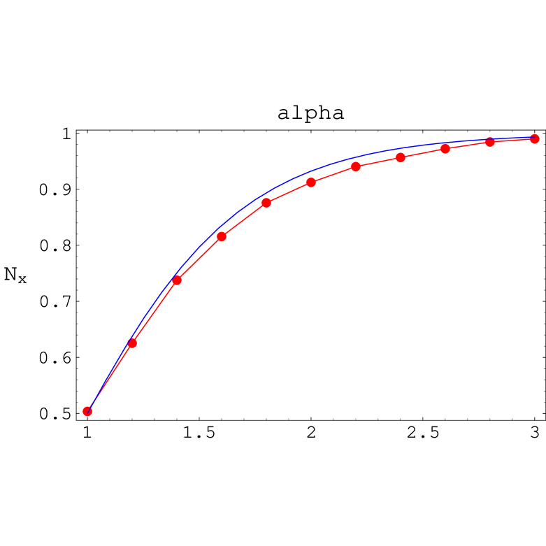
The final result (81) is in good, but not perfect, agreement with simulations. We believe that the only restriction on our method is that $D$ should be small, so that the method of steepest descent is appropriate. For $D=0.01$, the neglect of $O(D)$ corrections to (78) and (79) should mean that our result is within approximately 1% of the simulation results. It is not clear from an examination of Fig. 6 whether the slight discrepancy is due to the $O(D)$ corrections or to additional contributions which have not been accounted for. Since the agreement is still not perfect for smaller $D$, we should take the latter explanation seriously and carry out a search to see if we can find such additional terms. A possible source is the following. We have conjectured that the solution of (26) and (27) which has the least action can be obtained first by finding the $x_{c}(t)$ solution with $y_{c}=0$, and then linearizing about it. However, there are undoubtedly higher action solutions of (26) and (27) which have a non-trivial structure in $x$ and $y$, that is, solutions which cannot be obtained as a simple expansion about the $y=0$ solution. In other applications of the steepest descent method, we would neglect these solutions as they would give contributions which were exponentially smaller than the contributions from the least action solutions, and thus be completely negligible for small $D$. However, in this problem, after integrating over $T$, the previously exponentially small contribution becomes a power law (see Eqn. (72)), or more precisely, $D$ divided by the a quantity related to the action of the solution, all raised to a power. Although we do not know what power the higher action solutions will be raised to without further analysis, it is clear that solutions to (26) and (27) with, for instance, twice the action of the solution considered in this paper, have at least the potential of changing our result by a not insignificant amount. Thus it appears that the neglect of higher action solutions, which is common in most problems involving optimal paths, may not be so well-founded in the situation which we are considering in this paper.

VII conclusions

In this paper we have presented the motivation, justification and calculational details of a method for determining the probabilities of various metastable states being selected for occupation, when an unstable state decays. Although, as we hope we have made clear, this is a widespread phenomenon, theoretical progress seems to have been hampered by a lack of sufficiently powerful tools with which to attack the problem. As a consequence, most studies were carried out some time ago on one-dimensional systems (or quasi-one-dimensional systems). Yet, these are actually the systems of least interest. The really interesting aspects of the problem arise in two or more dimensions, where the system can perform Brownian motion near an unstable state, and then select a final state through a mixture of randomness (noise) and dynamics (which will necessarily be non-linear in all non-trivial cases). It is this interplay of randomness and determinism, both essential to the process, which makes the problem so difficult.

Our main purpose in this paper has been to show how the use of path-integral techniques, and especially the notion of optimal paths, can be used to analyze this technically hard problem. In order to stress that relatively naive approaches are not able to capture much of the subtlety of this problem, we carried through what seemed to us the most simple-minded approach to the problem in two dimensions, and showed that it was not able to give satisfactory results. Although the extent of the agreement with numerical work is always open to interpretation, there were two features which signified that the naive method was defective. Firstly, there was no systematic way to proceed with the calculation; one was faced with ad hoc choices which had to be made at several junctures in the calculation. Secondly, the crude approximation (12) to the already unsystematic result (14), actually gives better agreement with simulations than (14) itself, which indicates the dubious nature of these results. It should also be borne in mind that the prediction that $N_{x}=1/2$ when $\alpha=\beta$ is assured by symmetry and that in almost all schemes $N_{x}\rightarrow 1$ as $\alpha$ gets very much larger than $\beta$, simply because the noise will have very little effect in this case. If we add to this the expectation that $N_{x}(\alpha)$ will be a smooth function, we see that even the most simple minded approximation cannot be expected to be too far out. These observations indicate that we should focus more on the systematics (or lack thereof) of the calculation, rather than getting perfect agreement with simulation data.

The nature of the optimal paths used in the treatment presented here is different from those in the more familiar problem of escape from one potential well to the other. In that situation it takes an exponentially large time ($\exp{\Delta V/D}$, where $\Delta V$ is the height of the barrier), to make the transition from one potential well to another, and this is reflected in the fact that the optimal paths are essentially of infinitely long duration ($T\rightarrow\infty$). In the problem studied in this paper we are focusing on phenomena on much shorter time scales: the decay of a state with no barrier to a metastable state. Any subsequent process (presumably a noise-activated escape to a different well, of the kind we have just discussed) is of no interest to us here. Actually, as explained in Sec. II, we do not even ask that the end point of the optimal path is a metastable state, but only that it lies somewhere in the valley which leads to the metastable state in the full problem. The optimal paths in these cases are of finite duration. To achieve this, the initial velocity of the particle in the mechanical analogy has to be non-zero at the origin. As $T$ increases this initial velocity decreases, and eventually tends to zero if $T$ tends to infinity.

Many of the other details of the calculation involving optimal paths turn out to be remarkably subtle. For example, the use of the reduced potential simplifies the problem, but eliminating the actual minima means that we have to specify an arbitrary final value of $x$ (if we are considering state-selection into the positive $x$-valley), which we denote by $X$. However, the probability of the positive $x$-valley being selected should not depend on $X$, as long as $X$ has a value which lies in the valley. Reassuringly, this is what we find in our calculation, but it requires us to take into account the $y$-dependence of the path for this “common-sense” condition to be observed. In our earlier treatment[1], we sought to give only the outline of our method, and made the assumption that the total probability flux through a particular valley was proportional to (a) its value on the axes, and (b) its maximum value, which occurs at $T=T^{*}$ — the time for which $P(X,0,0|\vec{0},0)$ is a maximum at a fixed $X$. Within this scheme there was no way of determining $X$ and $Y$, and so we fixed them to our simulation results. The best values were $X\gtrsim X_{\rm min}$ and $Y\gtrsim Y_{\rm min}$, in line with our expectations. However, we have found here that it is possible to get a form for the $y$-component of the optimal path only if we assume that $X$ is sufficiently large — which comes from the requirement that $T$ must be sufficiently large — and so setting $X\approx X_{\rm min}$ and $Y\approx Y_{\rm min}$ is not possible in the approach we have adopted here. Needless to say, we expect that if we were able to find the full solution for the optimum path, then we would not need to constrain $X$ or $Y$ to be large: the expressions for the fluxes ${\cal F}_{x}$ and ${\cal F}_{y}$ would be valid for all $X\geq X_{\rm min}$ and for all $Y\geq Y_{\rm min}$. Presumably the fact that ${\cal F}_{x}$ decreases from its value at $X=X_{\rm min}$, and only becomes constant when $X$ equals a few $X_{\rm min}$, is not due to a violation of flux conservation (this would necessitate some flux leakage, and it is difficult to see where it would go to), but instead to the inapplicability of our calculational scheme for small $X$, which simply gives the incorrect expression for ${\cal F}_{x}$. It should be stressed that this is not a problem for our method: we simply take $X$ and $Y$ large enough so that ${\cal F}_{x}$ and ${\cal F}_{y}$ respectively, do tend to asymptotic values. These are the required values and are those which we use in our determination of $N_{x}$ and $N_{y}$.

An even more subtle aspect of the calculation concerns the applicability of the linear approximation in determining the $y$-component of the optimal path. Although at first sight $y_{c}(t)$ is not small for large $X$, it turns out that the range of final values of $y_{c}(t)$, denoted by $y_{f}$, decreases so fast as $X$ increases, that the small $y_{c}(t)$ approximation is still valid. Put more intuitively: if $T$ is large, the path has to take a wide detour to large $y$ if it is to take sufficiently large time to reach $(X,y_{f})$ (recall that $T$ is fixed for these paths). But “large $y$” means large relative to $y_{c}(T)=y_{f}$, and, as discussed earlier, the current ${\cal J}_{x}(X,y_{f},T)$ is effectively non-zero only for tiny values of $|y_{f}|$. So while it is true that on the scale of $y_{f}$ the excursions of the optimal path spread deep into the plane, in fact the range of $y_{f}$ is so minute, that the linearization assumption remains valid. The result that the probability is so concentrated about the axes is used in other places in the calculation. For example, in Sec. VI we argued that the “volume” integral in (67) could be replaced by the “surface” integral in (68), and then we proceeded to ignore some of the contributions from the “surfaces” in the later integral. We specified the volume in the case of the positive $x$-valley as the entire plane to the right of the line $x=X$. Actually, this is not quite correct, since we need to define a similar volume for the $y$-valleys, and these will overlap in the sectors where $x$ and $y$ are both large. We can be reasonably vague about how precisely to define these volumes and surfaces simply because ${\cal J}_{x}$ (and ${\cal J}_{y}$) fall away so fast that they have an utterly negligible contribution however we define them. In any reasonable definition, the only contribution to the surface integral (68) will be on the line $x=X$, very close to the $x$-axis.

We believe that one of the best indicators of the correctness of our approach is the cancellation of the various factors of $X$ coming from several different sources: (a) the fluctuations about the $y_{c}(t)$-solution, (b) the action of the $y_{c}(t)$-solution (after integration over $y_{f}$), (c) the action of the $x_{c}(t)$-solution (after integration over $T$), and (d) the definition of the current in terms of the probability distribution. What remains after these cancellations is essentially independent of $X$, as would intuitively be expected. As we have repeatedly stressed, many of these contributions come from assuming that $T$ is large. This seems somewhat paradoxical, since we would expect that state selection is determined at earlier times. This can be understood if one realizes that the large $X$ calculation determines the normalization of the flux in (73), or equivalently, the quantity $\zeta(\alpha,\beta)$ in (81). To obtain a finite $X\rightarrow\infty$ limit, it is essential to include a non-trivial $y_{c}(t)$ optimal path in the analysis. If the optimal path is taken to be $y_{c}(t)=0$, then only the $\tilde{D}^{\sigma}$ factor in (81) is determined. This was essentially the approach we adopted in our earlier paper[1]. While we believe that the treatment given here is a great improvement on that reported in Ref. [1], there is no doubt room for further improvement. For instance, the linearization approximation seems very reasonable on physical grounds, but it would be useful to put it on a sounder mathematical footing. A deeper understanding of the origin of the small scale set by $\exp{(-\gamma X^{2}/\alpha)}$ would also be valuable.

The competition between new modes, when a previously stable mode becomes unstable, is responsible for much of the emergent order found in systems far from equilibrium. The continual branching to more complex structures that this entails[30], is not only governed by the dynamics of the process but also by the random fluctuations, or noise, generated by the large number of other degrees of freedom of the system not explicitly included in the description. The model which we have investigated in this paper is, as has already been emphasized, the simplest showing enough of the complicated features of this process of state selection to serve as an illustrative example of our method. In forthcoming papers we will show how the method can be applied to more complex examples, such as state selection in lasers and the study of population dynamics in a fluctuating environment. We believe that the ideas and techniques developed here will not only be applicable to these situations, but to many others where multiple states compete for occupation.

A

In this appendix, we explore the consequences of the elementary theory put forward at the end of Sec. III. We will obtain simple expressions for the probability that the particle ends up in an $x$-valley, which are compared to Monte Carlo simulations in Sec. III.

We begin with the first ingredient in this simple theory. Since $\gamma=0$ we have only to solve the Langevin equations $\dot{x}=\alpha x+\eta_{x}(t)$ and $\dot{y}=\beta y+\eta_{y}(t)$. Such linear problems can always be exactly solved. Since $x$ and $y$ are linearly related to $\eta_{x}$ and $\eta_{y}$, they are also Gaussian random variables. It is easy to show that $\langle x(t)\rangle=\langle y(t)\rangle=0$ and therefore the probability that the particle is at $(x,y)$ at time $t$, given that it started at the origin at time $t=0$ is

$$P(x,y,t|0,0,0)={\cal N}\exp\left\{-\frac{x^{2}}{2\langle x^{2}(t)\rangle}-\frac{y^{2}}{2\langle y^{2}(t)\rangle}\right\}\,,$$ (A1)

where ${\cal N}$ is a normalization constant. For later use we will also need

$$\langle x^{2}(t)\rangle=\frac{D}{\alpha}\left(e^{2\alpha t}-1\right)\ \ ;\ \ \langle y^{2}(t)\rangle=\frac{D}{\beta}\left(e^{2\beta t}-1\right)\,,$$ (A2)

To quantify the second ingredient, first suppose that the coordinates of the particle $(x,y)$ are in the first quadrant. If the angle it makes with the positive $x$-axis, $\tan^{-1}(y/x)$ is less than $\tan^{-1}(Y_{\rm min}/X_{\rm min})$, then according to our criterion, it goes into the $x$-valley. Since the tan function is monotonic in the interval $(0,\pi/2)$, and generalizing to other quadrants by using $|x|$ and $|y|$ rather than $x$ and $y$, the criterion becomes:

$$\frac{|x|}{X_{\rm min}} > \frac{|y|}{Y_{\rm min}}\ \ \Rightarrow\ \ {\rm particle\ chooses\ }x{\rm-valley}$$ (A3)

$$\frac{|y|}{Y_{\rm min}} > \frac{|x|}{X_{\rm min}}\ \ \Rightarrow\ \ {\rm particle\ chooses\ }y{\rm-valley}\,.$$ (A5)

These ingredients can now be put together. The question reduces to how often the particle is in the sector specified by (A3) at a given time $t$ and how often it is in the sector specified by (A5) at this time. This probability is found by integrating (A1) over all $x$ and all $y$ with the constraint that it satisfies either (A3) or (A5) depending on whether we want the probability of ending up in the $x$-valley or $y$-valley. Restricting ourselves to the positive quadrant, which we can obviously do on symmetry grounds, the probability of ending up in an $x$-valley, $N_{x}$ and in a $y$-valley, $N_{y}$, are

$$N_{x} = 4{\cal N}\int^{\infty}_{0}dx\,\int^{\lambda x}_{0}dy\exp\left\{-\frac{x^{2}}{2\langle x^{2}(t)\rangle}-\frac{y^{2}}{2\langle y^{2}(t)\rangle}\right\}\ \ {\rm and}$$ (A6)

$$N_{y} = 4{\cal N}\int^{\infty}_{0}dy\,\int^{\lambda^{-1}y}_{0}dx\exp\left\{-\frac{x^{2}}{2\langle x^{2}(t)\rangle}-\frac{y^{2}}{2\langle y^{2}(t)\rangle}\right\}\,,$$ (A8)

where the factor $4$ comes from including the contributions from the other quadrants and $\lambda=Y_{\rm min}/X_{\rm min}$. In the $N_{x}$ integral, change variables from $y$ to $z$ where $y=\lambda xz$ at fixed $x$. The $x$ integral can now be easily performed, giving

$$N_{x}=4{\cal N}\frac{Y_{\rm min}}{X_{\rm min}}\langle x^{2}(t)\rangle\int^{1}_{0}\frac{dz}{1+\kappa^{2}(t)z^{2}}\,,$$ (A9)

where

$$\kappa^{2}(t)=\frac{\lambda^{2}\langle x^{2}(t)\rangle}{\langle y^{2}(t)\rangle}=\frac{Y^{2}_{\rm min}\langle x^{2}(t)\rangle}{X^{2}_{\rm min}\langle y^{2}(t)\rangle}\,.$$ (A10)

In a similar way

$$N_{y}=4{\cal N}\frac{X_{\rm min}}{Y_{\rm min}}\langle y^{2}(t)\rangle\int^{1}_{0}\frac{dz}{1+\kappa^{-2}(t)z^{2}}\,.$$ (A11)

From (A2) we see that if $\alpha$ and $\beta$ are not very different from each other, then $\kappa(t)$ will be neither very large nor very small, and we can ignore the integrals in (A9) and (A11) as a first approximation. Then determining ${\cal N}$ by asking that $N_{x}+N_{y}=1$ and ignoring the factor $1$ compared to the exponentials in (A2) yields

$$N_{x}=\frac{e^{2\alpha t}}{e^{2\alpha t}+e^{2\beta t}}\ \ ;\ \ N_{y}=\frac{e^{2\beta t}}{e^{2\alpha t}+e^{2\beta t}}\,.$$ (A12)

There are several simple arguments which give formulas resembling this. It is not difficult to improve on this by including the integrals in (A9) and (A11). Once again determining ${\cal N}$ by normalization gives

$$N_{x}=\frac{2}{\pi}\tan^{-1}[\kappa(t)]\ \ ;\ \ N_{y}=\frac{2}{\pi}\tan^{-1}[\kappa^{-1}(t)]\,,$$ (A13)

where we have used the result $\tan^{-1}(w)+\tan^{-1}(1/w)=\pi/2$. If $\langle x^{2}(t)\rangle\gg\langle y^{2}(t)\rangle$ or $\langle y^{2}(t)\rangle\gg\langle x^{2}(t)\rangle$, which can happen even when $\alpha$ and $\beta$ are not too different, we may replace (A13) by a simpler form which resembles (A12), but with constants multiplying the exponentials.

The simple result (A12) does not depend on the parameter $\gamma$, which represents the non-linear part of the potential, or on the noise strength, $D$. This is also true of (A13) if we ignore the factor $1$ compared to the exponentials in (A2). To understand this, let us suppose that $\alpha>\beta$. From (A12) or (A13), we see that when $t$ is small although there is a slight bias in favor of the $x$-valley over the $y$-valley, it is not that marked. However, as $t$ increases the asymmetry becomes more marked, until at large times the particle has only a very small chance of being in the $y$-valley. We need to simulate the role that the saddle points play in state selection by choosing the time to have the value $t_{c}$, which is the time at which it is most likely that the $x$ and $y$ coordinates of the particle will have magnitudes $X_{\rm min}$ and $Y_{\rm min}$ respectively. This is implemented by asking that $\langle x^{2}(t_{c})\rangle=X^{2}_{\rm min}$ or $\langle y^{2}(t_{c})\rangle=Y^{2}_{\rm min}$. Note that we have used the word “or”, since only one relation is required to determine $t_{c}$, and the two relations given give incompatible values for $t_{c}$ unless $\alpha=\beta$. Once again, as is common in many aspects of the naive approach to state selection which we have been summarizing in this appendix, there is a considerable degree of arbitrariness in the choice of $t_{c}$. We will assume that for $\alpha>\beta$, when the particle is most likely to go into the $x$-valley, $t_{c}$ is determined from the condition on $\langle x^{2}(t_{c})$ and vice-versa. Then from (A2),

$$t_{c}=-\frac{1}{2\alpha}\ln\left(\frac{\gamma D}{\alpha\beta}\right)\ \ ;\ \ \alpha\geq\beta,$$ (A14)

which has the characteristic form $-\ln D$ as $D\rightarrow 0$.

If we substitute (A14) into (A12) we obtain the probability of ending up in an $x$-valley. In terms of the quantities

$$\hat{D}\equiv\frac{\gamma D}{\alpha\beta}\ \ {\rm and}\ \ \rho=\frac{(\alpha-\beta)}{\alpha}\,,$$ (A15)

we obtain

$$N_{x}=\frac{1}{1+\hat{D}^{\rho}}\,.$$ (A16)

If we substitute (A14) into (A13) we obtain the more general form

$$N_{x}=\frac{2}{\pi}\tan^{-1}\hat{D}^{-\rho}\,.$$ (A17)

Equations (A16) and (A17) are the principal results of this appendix. The two main points we wish to make is (i) their derivation is somewhat arbitrary — there are several other similar assumptions we could make which would give us slightly different formulas, and (ii) although, as is discussed in Sec. III, they show the right qualitative features, they are are not in good agreement with Monte Carlo simulations. Thus a more systematic and sophisticated theory is required. This is given in Secs. IV, V and VI of the paper.

B

The purpose of this appendix is to explore the solution of (32), where $x(t)$ is given by (33) and where $y(0)=0$ and $y(T)=y_{f}$. Throughout we will assume that $T$ is large in the sense that $e^{-\alpha T}\ll 1$ and $e^{-\beta T}\ll 1$, which will allow us to obtain a rather simple form for the solution.

Small $t$ solution. Let $\zeta=X^{2}{\rm cosech}^{2}\alpha T$. Since $e^{-\alpha T}\ll 1$, $\zeta\ll 1$. Therefore (32) becomes

$$\ddot{y}=y\{\beta^{2}-2\zeta\gamma(\alpha+\beta)\sinh^{2}\alpha t+O(\zeta^{2})\}\,.$$ (B1)

We look for a solution of (B1) as a power-series in $\zeta$:

$$y(t)=y_{0}(t)+y_{1}(t)\zeta+O(\zeta^{2})\,.$$ (B2)

Clearly the zeroth-order solution which satisfies $y(0)=0$ is $y_{0}(t)=A\sinh\beta t$, where $A$ is an arbitrary constant. It is straightforward to determine $y_{1}(t)$, but since a short analysis shows that $y_{1}(t)\zeta\ll y_{0}(t)$ for all $t\lesssim T/2$, we conclude that, it is sufficient to take the small $t$ of the solution of (32) — which we denote by $y_{<}$ — to be

$$y_{<}(t)=A\sinh\beta t\ \ ;\ \ t<t_{m}$$ (B3)

Large $t$ solution. In this regime both $e^{-\alpha T}\ll 1$ and $e^{-\alpha t}\ll 1$, and therefore $x_{c}^{2}(t)$ and $x_{c}^{4}(t)$ may be approximated by $X^{2}e^{-2\alpha(T-t)}$ and $X^{4}e^{-4\alpha(T-t)}$ respectively. Using these forms in (32) and making the change of variables

$$z=\frac{\gamma X^{2}}{\alpha}\,e^{-2\alpha(T-t)}\ \ ;\ \ f=e^{z/2}\,z^{-\beta/2\alpha}y\,,$$ (B4)

we find that $f(z)$ satisfies the equation

$$z\frac{d^{2}f}{dz^{2}}+(\nu-z)\frac{df}{dz}=0\ \ ;\ \ \nu=\frac{(\alpha+\beta)}{\alpha}\,.$$ (B5)

This equation is easily solved to give

$$f(z)={\cal A}+{\cal B}\int^{\gamma X^{2}/\alpha}_{z}dz\,z^{-\nu}\,e^{z}\,,$$ (B6)

where ${\cal A}$ and ${\cal B}$ are arbitrary constants and where the upper limit of the $z$-integral has been arbitrarily chosen to be the value that $z$ takes on when $t=T$.

We now have to match (B6) to (B3) at $t=t_{m}$. It will turn out that we do not have to specify $t_{m}$ precisely, but let us assume for now that it has the value $T/2$. Then the corresponding value of $z$, $z_{m}$ is seen from (B4) to be very small. Formally the matching procedure consists of equating both $y(t_{m})$ and $\dot{y}(t_{m})$ for the solutions in the large and small time regimes. We will carry out this procedure below. However, let us first give a quick argument which gives us the correct final result.

For $t$ near $t_{m}$, $y_{<}(t)\sim A\,e^{\beta t}/2$. Also from (B4), $y_{>}(t)=e^{\beta t}\,e^{-z/2}\,f(z)$, and since $z_{m}\ll 1$, it follows that for $t$ near $t_{m}$, $y_{>}(t)\sim e^{\beta t}\,f(z)$. To get a smooth match, we require $f(z)$ to be a constant, $A/2$, for values of $z$ near $z_{m}$. Looking now at (B6), we see that the first term is constant, but the second term changes very quickly in the small $z$ regime, since it diverges in the $z\rightarrow 0$ limit. We therefore take ${\cal B}=0$ to get a smooth match, which in turn gives ${\cal A}=A/2$. Therefore

$$y_{>}(t)=\frac{A}{2}\,e^{\beta t}\,\exp\left\{-\frac{\gamma X^{2}}{2\alpha}\,e^{-2\alpha(T-t)}\right\}\ \ ;\ \ t>t_{m}\,.$$ (B7)

Having matched (B3) and (B7) near $t_{m}$, we can now fix the constant $A$ from the boundary condition $y(T)=y_{f}$. Doing this gives us the form (34).

Let us briefly indicate how we arrive at this result in a more systematic fashion. We can choose to either match $\{f(z),f^{\prime}(z)\}$ at $z=z_{m}$ or $\{y(t),\dot{y}(t)\}$ at $t=t_{m}$. They are related by

$$e^{-\beta t}\,y(t) = e^{-z/2}\,f(z)\ \ {\rm and}$$ (B8)

$$\frac{\dot{y}(t)}{y(t)}=\beta - \alpha z+2\alpha z\frac{f^{\prime}(z)}{f(z)}\,.$$ (B9)

Now, by successive integration by parts, we can obtain an approximation to the integral in (B6) valid for small $z$. For our purposes we need retain only the first term:

$$f(z)\approx{\cal A}+{\cal B}\,\frac{z^{-\nu+1}\,e^{z}}{\nu-1}\ \ ;\ \ z\approx z_{m}\,.$$ (B10)

Therefore to leading order

$$f_{>}(z_{m}) = {\cal A}+{\cal B}\,\frac{\alpha z_{m}^{-\beta/\alpha}\,e^{z_{m}}}{\beta}\ \ {\rm and}$$ (B11)

$$f_{>}^{\prime}(z_{m}) = -{\cal B}\,e^{z_{m}}\,z_{m}^{-(\alpha+\beta)/\alpha}\,.$$ (B12)

On the other hand $y_{<}(t_{m})=(A/2)e^{\beta t_{m}}$ and $\dot{y}_{<}(t_{m})=(\beta A/2)e^{\beta t_{m}}$. So from (B8) and (B9)

$$f_{<}(z_{m})=\frac{A}{2}e^{z_{m}/2}\ \ ;\ \ f_{<}^{\prime}(z_{m})=\frac{A}{4}e^{z_{m}/2}\,.$$ (B13)

Matching (B12) and (B13) gives

$${\cal A}=\frac{A}{2}\left[1+O(z_{m})\right]\ \ ;\ \ {\cal B}=\frac{A}{4}\,z_{m}^{(\alpha+\beta)/\alpha}\,\left[1+O(z_{m})\right]\,.$$ (B14)

Substituting (B14) into (B6) we obtain

$$f_{>}(z)=\frac{A}{2}\,\left\{1-z_{m}^{(\alpha+\beta)/\alpha}\,\int^{\gamma X^{2}/\alpha}_{z}dz\,z^{(\alpha+\beta)/\beta}\,e^{z}\right\}\,.$$ (B15)

Clearly for values of $z$ that are not small, the second term is completely negligible and so $f_{>}(z)\sim A/2$ to a very good approximation. However, even for values of $z$ near to $z_{m}$ we can neglect this term — it gives a contribution which is $O(z_{m})$. Therefore, once again, we obtain (B7).

In determining the form of $y(t)$, we have implicitly assumed that the solution of least action is such that $y(t)\neq 0$ for $t\neq 0$. However, there are other solutions of the type $y(t)=0$, for $t\leq t_{1}$, (where $t_{1}<T$) and a non-trivial solution of (32), where $x(t)$ is given by (33) and where $y(t_{1})=0$ and $y(T)=y_{f}$, for $t\geq t_{1}$. Intuitively, we would expect that the solution with $t_{1}=0$, which is the one found above, is the solution of least action, and all those with $t_{1}>0$ have greater action. This is due to the fact that, especially for large $t_{1}$, the path will have to sharply curve away from the $x$-axis if it is to satisfy the condition at $t=T$. We have checked this by numerically solving the differential equation (32) for $y(t)$ with different $t_{1}$ values, and found that the action monotonically increases with $t_{1}$.

Let us end by outlining the evaluation of the classical action (36). To evaluate $E$ we choose to take $t=0$, since in this case $U=0$. Also $V|_{t=0}=0$ and $V|_{t=T}=-\frac{1}{2}\alpha X^{2}+\frac{1}{2}y_{f}^{2}[\gamma X^{2}-\beta]$. Therefore

$$S_{c} = \left\{\frac{1}{2}\int^{T}_{0}dt\,\dot{x}^{2}_{c}-\frac{1}{4}\left.\dot{x}^{2}_{c}\right|_{t=0}\,T-\frac{1}{4}\alpha X^{2}\right\}$$ (B16)

$$+ \left\{\frac{1}{2}\int^{T}_{0}dt\,\dot{y}^{2}_{c}-\frac{1}{4}\left.\dot{y}^{2}_{c}\right|_{t=0}\,T+\frac{1}{4}y_{f}^{2}[\gamma X^{2}-\beta]\right\}\,.$$ (B17)

The first bracket on the right-hand side of (B17) is easily evaluated from $x_{c}(t)$ given by (33). One finds $(\alpha X^{2}/4)({\rm coth}\alpha T\,-1)$. The second bracket requires a little more calculation, since $y_{c}(t)$ has a different functional form depending on whether $t$ is less than, or greater than, $t_{m}$. Substituting the form for $t\leq t_{m}$ first of all, gives for the second bracket:

$$\frac{1}{2}\int^{T}_{t_{m}}dt\,\dot{y}^{2}_{c}+\frac{A^{2}\beta}{8}\sinh 2\beta t_{m}-\frac{A^{2}\beta^{2}}{4}\left(T-t_{m}\right)+\frac{1}{4}y_{f}^{2}[\gamma X^{2}-\beta]\,.$$ (B18)

Using (34) and changing variables from $t$ to $z$ (given by (B4)) one finds

$$\frac{1}{2}\int^{T}_{t_{m}}dt\,\dot{y}^{2}_{c}(t)=\frac{A^{2}}{16\alpha}\,\left(\frac{\alpha}{\gamma X^{2}}\right)^{\beta/\alpha}e^{2\beta T}\,\int^{\gamma X^{2}/\alpha}_{z_{m}}dz\,z^{(\beta/\alpha)-1}\,e^{-z}\,(\beta-\alpha z)^{2}\,.$$ (B19)

The range of the integral in (B19) may be taken as $(0,\gamma X^{2}/\alpha)$ as long as we subtract out

$$\int^{z_{m}}_{0}dz\,z^{(\beta/\alpha)-1}\,e^{-z}\,(\beta-\alpha z)^{2}=\alpha\beta z_{m}^{\beta/\alpha}\,\left[1+O(z_{m})\right]\,.$$ (B20)

The upper limit in the integral in (B19) is $O(1)$, and therefore the integral itself is also $O(1)$. Therefore the contribution (B20) is negligible compared to it, and so we may effectively replace the lower limit of the integral in (B19) by zero. The third term in (B18) being linear in $(T-t_{m})$ is negligible compared with the second term which is exponential in $2\beta t_{m}$. This term is in turn negligible compared to (B19), since $e^{-2\beta(T-t_{m})}\ll 1$. So the leading contribution to (B19) is

$$\frac{1}{4}y_{f}^{2}[\gamma X^{2}-\beta]+\frac{A^{2}}{16\alpha}\,\left(\frac{\alpha}{\gamma X^{2}}\right)^{\beta/\alpha}e^{2\beta T}\,\int^{\gamma X^{2}/\alpha}_{0}dz\,z^{(\beta/\alpha)-1}\,e^{-z}\,(\beta-\alpha z)^{2}\,.$$ (B21)

Substituting the value of $A$ determined from the boundary condition $y(T)=y_{f}$, into (B21), the classical action (B17) becomes

$$S_{c} = \frac{\alpha X^{2}}{4}\,({\rm coth}\alpha T\,-1)+\frac{1}{4}y_{f}^{2}[\gamma X^{2}-\beta]$$ (B22)

$$+ \frac{y_{f}^{2}}{4\alpha}\,\left(\frac{\alpha}{\gamma X^{2}}\right)^{\beta/\alpha}\,\exp\left\{\frac{\gamma X^{2}}{\alpha}\right\}\,\int^{\gamma X^{2}/\alpha}_{0}dz\,z^{(\beta/\alpha)-1}\,e^{-z}\,(\beta-\alpha z)^{2}\,.$$ (B23)

REFERENCES

- [1] M. B. Tarlie and A. J. McKane, J. Phys. A31, L71 (1998).
- [2] L. Segel, J. Fluid Mech. 14, 97 (1962); A. Newell and J. Whitehead, J. Fluid Mech. 38, 279 (1969).
- [3] R. Graham, Phys. Rev. A10, 1762 (1974).
- [4] L. Kramer and W. Zimmermann, Physica D 16, 221 (1985).
- [5] L. Kramer, H. R. Schober and W. Zimmermann, Physica D 31, 212 (1988).
- [6] B. Bagchi and G. R. Fleming, J. Phys. Chem. 94, 9 (1990).
- [7] C. S. Poornimadevi and B. Bagchi, Chem. Phys. Lett. 168, 276 (1990).
- [8] R. Roy and L. Mandel, Opt. Comm. 34, 133 (1980).
- [9] M. Sargent, M. O. Scully and W. E. Lamb, Laser Physics (Addison-Wesley, Reading, Mass., 1974).
- [10] E. C. Pielou, Mathematical Ecology (Wiley, New York, 1977). Second edition.
- [11] R. M. May, Model Ecosystems (Princeton University Press, Princeton, N.J, 1973). Chapter 5.
- [12] For a review, see Y. Liu and M. Suzuki, Phase Transitions, 10, 303 (1987).
- [13] U. Weiss, Phys. Rev. A25, 2444 (1982).
- [14] T. Kunisawa and J. Otsuka, Prog. Theo. Phys. 67, 804 (1982).
- [15] H. Dekker, Phys. Lett. A88, 279 (1982).
- [16] V. F. Baibuz, V. Y. Zitserman and A. N. Drozdov, Physica A127, 173 (1984).
- [17] G. Hu, Phys. Lett. A116, 361 (1986).
- [18] M. O. Hongler and R. C. Desai, Hel. Phys. Acta 59, 367 (1986).
- [19] R. Phythian and W. D. Curtis, J. Stat. Phys. 46, 217 (1987).
- [20] F. T. Arecchi, A. Politi and L. Ulivi, Phys. Lett. A87, 333 (1982).
- [21] M. R. Young and S. Singh, Phys. Rev. A31, 888 (1985).
- [22] R. Phythian and W. D. Curtis, Physica A169, 292 (1990).
- [23] F. Haake, J. W. Haus and R. Glauber, Phys. Rev. A23, 3255 (1981).
- [24] M. Mangel, Phys. Rev. A24, 3226 (1981).
- [25] M. B. Tarlie and K. R. Elder, Phys. Rev. Lett. 81, 18 (1998).
- [26] J. Zinn-Justin, Quantum Field Theory and Critical Phenomena (OUP, New York, 1996).
- [27] M. Abramovitz and I. A. Stegun (eds), Handbook of Mathematical Functions (Dover, New York, 1965).
- [28] See, for instance, A. J. McKane and M. B. Tarlie, J. Phys. A28, 6931 (1995).
- [29] H. Risken, The Fokker-Planck Equation (Springer-Verlag, Berlin, 1989). Second edition.
- [30] F. Arecchi, Ann. N.Y. Acad. Sci. 879, 45 (1999). Section 4.