Slow dynamics and aging in a non-randomly frustrated spin system

Abstract

A simple, non-disordered spin model has been studied in an effort to understand the origin of the precipitous slowing down of dynamics observed in supercooled liquids approaching the glass transition. A combination of Monte Carlo simulations and exact calculations indicates that this model exhibits an entropy vanishing transition accompanied by a rapid divergence of time scales. Measurements of various correlation functions show that the system displays a hierarchy of time scales associated with different degrees of freedom. Extended structures, arising from the frustration in the system, are identified as the source of the slow dynamics. In the simulations, the system falls out of equilibrium at a temperature $T_{g}$ higher than the entropy-vanishing transition temperature and the dynamics below $T_{g}$ exhibits aging as distinct from coarsening. The cooling rate dependence of the energy is also consistent with the usual glass formation scenario.

I Introduction

The exact nature of the glass transition in supercooled liquids is still an enigma. The hallmark of this transition is a precipitous slowing down of the dynamics without any accompanying, obvious, structural changes[1, 2]. The analogous transition in spin glasses, which have quenched randomness, is much better understood and the theoretical understanding in that field has benefitted from the existence of simple microscopic models[3]. A search for models which do not have disorder at the microscopic level but display glassy dynamics has been one of the important directions of current research. In this paper, we present a detailed analysis of a non-disordered spin model whose phenomenology is remarkably similar to that of supercooled liquids. The model can be solved exactly in a certain limit[4], and the exact results can be related to the glassy dynamics observed in simulations of the model. This connection can be exploited to address the issue of the origin of the rapid divergence of time scales[5] in supercooled liquids.

It is well known that relaxation times diverge at a critical point[6], however, unlike critical points, there is no obvious length-scale divergence that has been associated with the glass transition. Recent experiments[2, 7, 8] and simulations[9] point toward the existence of dynamical heterogeneities[2, 7, 8] and a time-dependent length scale[9] which grows as the glass transition is approached. This raises the question of whether the occurrence of a critical point is responsible for the anomalously slow relaxations observed in glasses, and if so what is the nature of this critical point. A scenario proposed by Adam,Gibbs and DiMarzio is that glassy dynamics is associated with an underlying configurational entropy vanishing transition [10, 11]. The slow relaxation is due to the small equilibrium entropy near glass transition temperature and the growing length-scale is associated with cooperatively relaxing regions. This theory is compatible with Kauzmann’s entropy crisis argument[12], which predicts a lower limit of the glass transition temperature and is supported by experiments measuring configurational entropy in the glass forming liquids[13]. In recent years, this scenario has been explicitly realized in p-spin spin glasses as a random first order transition[14, 15, 16, 17]. Based on an inherent structures approach[18], indications of a similar scenario have been found in simulations of Lennard-Jones systems[19]. Another possibility that has been suggested to reconcile the observed time-scale divergence with no apparent length scale divergence is the existence of a zero-temperature critical point[20] which has characteristics similar to the critical point in a random-field Ising model[21]. A major obstacle in obtaining definitive answers is the identification of simple, non-disordered models where such scenarios are explicitly realized.

In recent years, studies have focused on microscopic models with no quenched disorder which exhibit glassy dynamics. Models in this category include a ferromagnetic four-spin plaquette model on a cubic lattice[22] which exhibits aging[23], three-dimensional Ising models with competing nearest and next-nearest neighbor interactions[24] exhibiting logarithmic growth. Besides these, there are constrained dynamics models, as for example, the two-dimensional ferromagnetic Ising model with three-spin interactions [25]. The presence of a critical point has not been related to the glassy dynamics in any of these models.

The model studied in this paper is the compressible, triangular-lattice, Ising antiferromagnet(CTIAFM)[26]. We will present results of a Monte Carlo(MC) simulation study of the dynamics in the supercooled state of CTIAFM and an exact solution in the limit of vanishing “thermal” fluctuations. The exact solution exhibits a critical point which is accompanied by a vanishing of configurational entropy. The model and its equilibrium behavior are discussed in section II. In section III, we introduce a mapping of the spin model to a geometrical model and the exact solution is discussed in section IV. In section V and VI, we present our MC study of the supercooled phase and the glass phase, respectively. Our conclusions are presented in section VII.

II CTIAFM model

The CTIAFM is a simple extension of the well known triangular-lattice Ising antiferromagnet(TIAFM)[27, 28]. The TIAFM is a fully frustrated model and has no finite temperature transition. The number of ground states is exponentially large, and the $T=0$ state is critical, characterized by a power law decay of spin correlation functions[29]. The critical ground state has been studied extensively by mapping to interface models[30, 31]. The effect of degeneracy-lifting fields on the TIAFM and the resulting possibility of phase transitions has also been the subject of many investigations[28, 30, 32, 33].

In CTIAFM, a coupling to elastic strain fields removes the degeneracy of the ground state[34]. In our current study only homogeneous strain fields are considered; the distortion is uniform and does not depend on the site. Thus, the additional degrees of freedom are encapsulated in three strain fields, {${e_{\alpha},\alpha=1..3}$}, in the Hamiltonian:

$$H=J{\sum}_{<ij>}S_{i}S_{j}-\epsilon J{\sum}_{\alpha}e_{\alpha}{\sum}_{<ij>_{\alpha}}S_{i}S_{j}+N{E\over 2}{\sum}_{\alpha}e_{\alpha}^{2}~{}.$$ (1)

Here $J$, the strength of the nearest-neighbor anti-ferromagnetic coupling, is modulated by the presence of the second term which defines a coupling between the spins and the strain fields {$e_{\alpha}$}. The coupling $\epsilon$ is chosen to be a positive constant to ensure that antiferromagnetic interaction gets stronger when spins get closer. The last term represents the elastic energy needed to stabilize the unstrained lattice and $N$ is the total number of lattice spins. This model can be thought of as a spin model with anisotropic couplings. The anisotropic couplings are determined by the strain fields and are, therefore, annealed variables as opposed to models with fixed (quenched) anisotropy[28, 30].

The phase transitions of this model were analyzed in the context of the effects of elastic strain fields on ordering transition in alloys[26]. This, and other previous studies, showed that the competition between energy and entropy leads to a first order transition at a finite temperature $T_{1}$[34, 35]. Above $T_{1}$, the system is in a disordered, paramagnetic state and the lattice is contracted isotropically in three directions. Below $T_{1}$, there is a lattice distortion and the spins order as stripes with alternating up and down rows: the ferromagnetic bonds are elongated, and antiferromagnetic bonds are contracted. The ordered state is six fold degenerate since up and down spins rows can alternate in any of the three nearest neighbor directions and the state also has the Ising up-down symmetry. Thus, the CTIAFM ground-state entropy density is zero. It has been argued that there is an instability to the lattice distortion at a temperature below $T_{1}$[34]. In the following section, we introduce a geometrical mapping which is valid for all spin configurations within the ground-state ensemble of the TIAFM and study phase transitions within this ensemble as the coupling to the strain fields is varied. The model can be exactly solved in this limit where excitations out of the TIAFM ground state, the “thermal” fluctuations, are neglected.

III String Picture– CTIAFM revisited

There is a well-known mapping of the ground states of the TIAFM on to string configurations[30, 33]. This string picture has proven to be extremely useful in understanding the behavior of the CTIAFM.

Any spin configuration belonging to the ground state of the TIAFM has two antiferromagnetic(satisfied) bonds and one ferromagnetic(unsatisfied)bond in every triangular plaquette. A dimer covering[33, 36] can be defined on the dual lattice for these spin states. The dimers are placed on the those bonds of the dual honeycomb lattice which connect the centers of triangles sharing an unsatisfied (ferromagnetic) bond. Since there is exactly one unsatisfied bond for every triangle, any site on the dual lattice is connected to exactly one dimer. The resulting dimer covering is unique. Fig.(1a) shows such a dimer covering for an arbitrary ground state. Under this dimer mapping, the spins in the striped phase define a dimer covering (Fig.(1b)), where all dimers are aligned in one direction (vertical in this example). Based on the dimer mapping, the ground states can be categorized into different sectors by superposing a dimer covering onto the standard dimer covering in Fig.(1b) where all dimers are vertical. The overlap defines linear structures. For example, the spin state in Fig.(1a) is mapped onto the string picture in Fig.(2a). Each string sector is characterized by a string number density $p=\frac{N_{s}}{L}$ where $N_{s}$ is the total number of strings and $L$ is system size. Under such mapping, the disordered paramagnetic states with the maximum number of free spins[29] correspond to $p=\frac{2}{3}$ and the striped ordered spin states correspond to $p=0$. For each string sector $p$, the total number of spin states can be enumerated by using a transfer-matrix technique[33]. The associated entropy density is a continuous function which peaks at $p=\frac{2}{3}$ and vanishes at $p=0$ (cf inset to Fig. 3).

The strings obtained from the TIAFM ground state spin configurations do not intersect. They run vertically through the system without being interrupted, therefore, the number of strings per row is conserved. Under periodic boundary conditions, strings wrap around and form loops. If the system is restricted to the TIAFM ground state ensemble, the number of strings does not change under any local dynamics(single or multiple spin flips or exchanges). Thus, spin states belonging to different string number sectors are completely disjoint. These string sectors are the inherent structures[18] of the TIAFM within any local dynamics: any spin configuration will relax to one of the string sectors under energy minimization.

Excitations out of the TIAFM ground state ensemble involve triangular plaquettes with all three spins pointing up or down. These plaquettes are topological defects at which the strings can end[30]. The TIAFM ground states and the associated dimer coverings can be mapped to an interface model with a scalar height variable[30, 31, 37] and the defects are dislocations in the height field. The height mapping can be used to demonstrate that the TIAFM ground-state is critical with power-law correlations and the defects form the basis of the Coulomb-gas representation of this model[30]. Defects play an important role in the dynamics of the strings[38]. Single spin flips or exchanges create defects in pairs which can then move away from each other. Each separated defect pair is connected by two strings. Thus, defects can increase or decrease the number of strings by two as they move toward or away from each other.

A previous Monte Carlo study has shown that when quenched below the first order transition temperature $T_{1}$ from the disordered phase, the CTIAFM exhibits a behavior remarkably similar to the phenomenology of the structural glass[35, 38]. For a range of supercooling temperatures, the system remains disordered and the supercooled phase is ergodic. Below a certain characteristic temperature $T^{*}$, however, the system freezes into a “glassy” phase. In this phase, the system becomes non-ergodic and the energy evolution is characterized by a step-wise relaxation which is history dependent.

In this work, we present an analytic solution of the CTIAFM within the ground-state ensemble of the TIAFM and show that the coupling to the elastic strain fields leads to a phase transition at which the string density vanishes discontinuously. We analyze the glassy dynamics observed in Monte Carlo simulations in terms of the string picture and the phase transitions occurring within the ground-state ensemble[4].

IV Phase transitions within the ground-state ensemble of the TIAFM

The string picture is rigorously defined when the spin states are restricted to the configurations without any defects. In the TIAFM, all these configurations have identical energies. In the CTIAFM, however, the energy of the state depends on the string density[4]. To see this, one integrates out the purely Gaussian strain fields in the CTIAFM Hamiltonian (Eq. 1) which yields an energy function with a four-spin coupling and a coupling parameter $\mu={\epsilon}^{2}{J}^{2}/E$:

$$H=J{\sum}_{<ij>}S_{i}S_{j}-(\mu/N){\sum}_{\alpha=1,2,3}({\sum}_{<ij>_{\alpha}}S_{i}S_{j})^{2}~{}.$$ (2)

The first term is identical for all configurations in the ground state ensemble, and can be neglected. The sum ${\sum}_{<ij>_{\alpha}}S_{i}S_{j}$, can be written in terms of the string density in the direction $\alpha$, i.e., the overlap of the dimers with a configuration where all dimers are pointing in the $\alpha$ direction. Under simple periodic boundary conditions, where each string wraps around only once around the system, two of the three string densities have to be equal. In addition, the constraint that there are two good bonds per triangular plaquette, leads to the condition that the sum of the three string densities have to add up to the numerical value of two. With these constraints, only one string density is independent and the energy per spin of the CTIAFM can be written as

$$H/N=-(\mu/2)[(1-2p)^{2}+2(1-p)^{2}]~{},$$ (3)

where $p$ is the one independent string density. Since the energy depends only on the string density and the entropy density for a given string density has been calculated exactly[33], the partition function of the model can be calculated exactly: $Z={\sum}_{p}\exp{(-N(\beta H(p)-\gamma(p)))}={\sum}_{p}\exp{(-Nf(p))}$. Here $\gamma(p)$ is the entropy per spin of the string sector with string density $p$[33] and $\beta$ is the inverse temperature. The sum over $p$ can be replaced by $\exp{(-Nf_{min}(p))}$ where $f_{min}(p)$ is $f(p)$ evaluated at the string density $p$ which minimizes the free-energy function $f(p)$. This free-energy function, which is exact if excitations out of the ground-state ensemble of the TIAFM are neglected, is shown in Fig (3). At small coupling constants, the free energy function shows a single global well at $p=\frac{2}{3}$. As the coupling constant is increased, a second minimum develops at $p=0$. A first order transition is expected at that value of the coupling constant where the two minima become degenerate. In our model the four-spin coupling is of infinite range and the barrier to nucleation is unsurmountable. If the system is initially in the $p=2/3$ state, it will remain indefinitely in this state. At a higher coupling constant, however, the $p=2/3$ state becomes unstable, as shown in Fig. (3). This is akin to a spinodal point[39] except that the order parameter is the string density which involves extended structures and is not the average of any local quantity. The instability of the $2/3$ state is also an entropy vanishing transition since the entropy of the $p=0$ state is zero.

Within the ground-state ensemble of the TIAFM, no local dynamics can change the density of strings. The entropy-vanishing transition can, therefore, be realized in two ways; (a) allowing for the system to explore states outside the ground-state ensemble by creating defects and (b) implementing a non-local dynamics which can change the string density without moving out of the ground-state ensemble. In this paper, we discuss the dynamics resulting from the first approach by allowing for the presence of a small density of defects. As will be discussed in the next section, we concentrate on analyzing the nature of the relaxations as the entropy-vanishing transition is approached without addressing the issue of whether this transition survives as a true thermodynamic transition in the presence of defects.

Before proceeding to the discussion of the simulations, we would like to point out that the the entropy-vanishing transition is akin to a zero-temperature critical point since the “thermal” fluctuations, in the form of defects, are frozen and play no role at the critical point. The relevant coupling is $\beta\mu$, the coupling to the elastic strain which controls the frustration[20]. This scenario is reminiscent of the zero-temperature critical point in the random-field Ising model[21] with $\beta\mu$ playing the role of the random field.

The exact solution can also be viewed in the context of inherent structures[18, 19] and shows that there is a phase transition involving these structures. At small values of $\beta\mu$, the inherent structures belong to the $p=2/3$ sector and the configurational entropy is finite. As $\beta\mu$ is increased, there is a thermodynamic instability of this sector leading to a change in the nature of the inherent-structure landscape. The set of inherent structures that are accessible to the system, thus, changes at the transition. As our simulations will show, this change can lead to an anomalous slowing down of the dynamics.

V Dynamics in supercooled phase

In this section we present a detailed discussion of the observed dynamics in the supercooled phase. To implement the local dynamics we used spin-exchange kinetic extended to include updates of the homogeneous strain fields[26]. For the Monte Carlo (MC) studies presented in this paper, a rhomboid system with periodic boundary conditions was chosen. Unless stated explicitly, the system size is 96x96. For all the measurements, the sampling is done every ten MC steps. The parameters of the Hamiltonian were chosen to be; $J=1$, ${\epsilon}=0.6$ and $E=2$. These imply a value of $\mu=0.18$ and the coupling constant $\beta\mu$ is controlled by the temperature of the MC simulation. In units of $\frac{J}{k_{B}}$ , the first-order transition temperature is $T_{1}=0.667$, and the entropy-vanishing transition temperature is $T^{*}=0.397$[4]. The defect density at temperatures close to the entropy vanishing transition, $T^{*}$, is around $0.04{\%}$[4]. We study this regime in order to investigate the possibility of the zero-defect critical point controlling the behavior at low but finite defect densities.

Dynamics of the supercooled phase was studied following instantaneous quenches from a random high-temperature disordered phase into a range of temperatures below $T_{1}$. After each quench, the system was equilibrated, and the time-history of various quantities were recorded, and auto-correlation functions were calculated. The evidence for diverging time scales has been presented earlier[4]. In this paper, we extend our analysis to the many different time scales observed and the relationship between them.

A Relaxations of strings and spins

The MC moves involve spin exchanges and updates of the strain fields. Updates in strain fields change the effective interaction between spins along the three nearest-neighbor directions and this is reflected in the update probabilities associated with the spin exchanges. Since the strain fields are homogeneous, these changes are global.

There are different classes of spins in the system. The free spins have equal numbers of antiferromagnetic and ferromagnetic bonds. They are represented as filled circles in Fig.2 and are located at kinks in the strings. Spin exchanges involving free spins lead to fluctuations of the strings. Exchanges involving spins located away from the kinks (which are not free) lead to the creation of defects. This is an activated process with an energy barrier of $4J$ in the absence of any homogeneous strains. The strain fluctuations change this value since the effective interactions become anisotropic and depend on the value of the strain fields. We found that the defect density can still be represented by an Arrhenius form with an “effective” barrier which is smaller than $4J$[40]. The two different classes of spins therefore have very different relaxation time scales with the free spins defining the shortest time scale in the system and the time scale associated with the defects growing in an Arrhenius fashion. The dynamics of the spins is, therefore, expected to be heterogeneous and controlled by the spatial distribution of strings.

The spatial distribution of the strings evolves in time as the strings diffuse across the system. Since the string density is the order parameter associated with the entropy-vanishing transition, this is expected to be the slowest mode in the system. The spins, therefore, respond to a quasi-static arrangement of the strings. This would lead us to expect non-exponential relaxations for the spins and the energy fluctuations (dominated by defect number fluctuations) since relaxation times depend on the proximity of the spins to the strings. Our simulation results are in qualitative agreement with these expectations.

The auto-correlation functions of the string density, $C_{string}(t)=<p(t)p(0)>-<p(t)>^{2}$, at different temperatures are shown in Fig.4. The correlations functions are seen to be exponentials, $\exp(-\frac{t}{\tau})$, with $\tau$ rapidly increasing as the temperature decreases. The time scales $\tau$ obtained from the fitting are plotted versus temperature in Fig.5. The two remarkable features of the string relaxation are (a) the exponential behavior with a single time scale and (b) the rapid increase of this time scale with an apparent divergence at a temperature close to $T^{*}$. We will discuss these features in the context of the entropy-vanishing transition after presenting the results for the defect, energy and spin relaxations. The rapid increase of the string-relaxation time scales, restricts our equilibrium measurements to temperatures $T\geq T_{g}\simeq 0.47$, the analog of the laboratory glass-transition temperature for our simulations.

The auto-correlation functions of the defect number, $C_{defect}(t)=<N_{d}(t)N_{d}(0)>-<N_{d}(t)>^{2}$ where $N_{d}$ is the total number of defects, are shown in Fig.6a. These functions are non-exponential and are best fit by stretched exponentials, $\exp(-\frac{t}{{\tau}_{d}})^{\beta}$, with a stretching exponent $\beta$ decreasing with temperature and a relaxation time $\tau$ increasing with temperature. The time-scale increase is Arrhenius (Fig 6b) with no apparent finite-temperature divergence. The stretching exponent approaches a value of $1/3$ as the temperature approaches $T_{g}$. This is consistent with a theory associating stretched exponential relaxations with random walks on a high-dimensional critical percolation cluster where the limiting value of $\beta=1/3$ is reached at percolation[41]. The energy relaxation (Fig (7)) also shows a stretched exponential form with a $\beta$ approaching $1/3$. Fig. (7) also shows the waiting-time ($t_{w}$) dependence of the correlations functions (cf. discussion in section VI). The relaxation times and stretching exponents are summarized in Table (I). The energy relaxation time shows a stronger divergence than the Arrhenius behavior of the defects, however, the absolute values of the time scales are orders of magnitude smaller than the string-relaxation times. The stretched exponential relaxation indicates that the energy and defect relaxations are reflecting the spatial heterogeneity imposed by the strings and their slow relaxation.

The spins are the basic microscopic entities in the system and the relaxations of the strings and defects get reflected in the spin relaxation. Spin auto-correlation functions at different temperatures are shown in Fig.8. These obey a power law decay with an exponential cutoff; $C(t)\simeq t^{\alpha}\exp{(-\frac{t}{{\tau}_{s}})}$. As $T_{g}$ is approached from above, the relaxation time ${\tau}_{s}$ increases exponentially and closely tracks the string relaxation time. The exponent $\alpha$ decreases with $T$ and the value is close to $1/4$ at $T=0.47$. The results from the fits are shown in Table (II). The exponent $\frac{1}{4}$ characterizes spin relaxation in the critical ground state of the pure TIAFM. This suggests that for times short compared to the string relaxation times, the spins respond as they would in the TIAFM ground state ensemble, except for the perturbation due to defect creation and annihilation; an effect that decreases with decreasing temperature.

The results of the simulations discussed above, show that there are multiple relaxation mechanisms in the supercooled state of the CTIAFM and that the spin and energy relaxations become increasingly non-exponential as the temperature approaches $T^{*}$. The slowest mode, the string-density, is characterized by a single time scale. The string density is the ‘order-parameter’ for the entropy-vanishing transition and the exponential relaxation is consistent with a mean-field transition. Since the strings are extended objects, their relaxations create a spatially heterogeneous environment for the local degrees of freedom, the spins and the defects, providing a mechanism for the stretched exponential relaxations. The observation of a stretching exponent similar to that appearing in the theory based on percolations clusters[41] is intriguing and suggests that the possibility of such a scenario occurring in the CTIAFM should be explored further.

We have argued that the entropy-vanishing transition at $T^{*}$ can lead to the anomalously slow dynamics observed in our simulations because the time scale of order-parameter relaxations diverges at this transition and because the order parameter involves extended objects which can create spatial heterogeneities. A remaining puzzle is the rapidly increasing time scale associated with the string-density relaxation. The rise in time scales is much faster than what would be expected from usual critical slowing down. This becomes evident upon comparing the increase of the static susceptibility (associated with the string density) which is expected to diverge at $T=T^{*}$, with the increase in time scales. In the temperature regime between 0.6 and 0.47, the static susceptibility increases by a factor of $2$ whereas the relaxation time increases by a factor of $\simeq 50$. As shown in Fig. 5, the rapid increase of $\tau$ can be described well with either the Vogel-Fulcher exponential increase[42] or a power law with a large exponent. We do not have an explanation of this anomalously fast increase of the time-scale, however, all our observations suggest that this is an intrinsic property of the entropy-vanishing transition and that the extended structures play a crucial role. Further evidence supporting the claim that the entropy vanishing transition has a different character than a usual mean-field critical point, was provided by a study of the fluctuations in string density over different time intervals.

B Distribution function of String Number Deviation

The nature of the string-density fluctuations was monitored by measuring the distribution of the string density difference $P({\Delta}p(t))$, where ${\Delta}p=p(t+t_{0})-p(t_{0})$ defines the deviation of the string density in the time $t$. The distribution is generated by choosing different time origins $t_{0}$. Fig.9 shows the distribution $P({\Delta}p)$ for $T=0.55$ and $T=0.47$. For high temperatures, both at short and long time intervals t, the distribution is close to a Gaussian. At $t=0$, $P({\Delta}p)$ is just a $\delta$ function peaking at ${\Delta}p=0$. As t increases, the width of the distribution gets broader. At some intermediate time, the non-Gaussian behavior becomes most prominent. After that, the distribution narrows down back to a Gaussian and reaches a stationary Gaussian distribution. At $T=0.55$, the distribution become most non-Gaussian at $t=4000$. As $T$ decreases, this intermediate time scale increases rapidly, and at $T=0.47$, the distribution becomes broader and broader with $t$, and the stationary distribution is not observed for times as long as $t=30,000$. According to the usual picture of the dynamics of a system near a critical point, the distribution of the order parameter difference is expected to become stationary at a time scale comparable to the relaxation time which increases rapidly as the critical point is approached[6]. The distribution is also expected to show significant non-Gaussian character at $T\sim T_{c}(L)$, where $L$ is the system size. To make a direct comparison, a measurement of the magnetization deviation, similar to the measurement of the string-density deviation, was undertaken for an Ising ferromagnet on a square lattice with $L=64$. The distribution of magnetization deviation at time interval $t$, $P(M(t_{0}+t)-M(t_{0}))$, was found to reach a stationary distribution for different $T$ as shown in Fig.10. It is evident that this behavior is different from what was observed for the strings. This difference between the strings relaxation behavior and that of the usual order parameter, however, is not reflected in $C_{string}(t)$. The equilibrium $C_{string}(t)$ can be directly related to the second moment of the distribution $P({\Delta}p(t))$ as:

$$<({\Delta}p(t))^{2}> = <(p(t)-p(0))^{2}>\ =\ 2<p^{2}>-2<p(t)p(0)>$$ (4)

$$= 2(<p^{2}>-<p>^{2})(1-\frac{<p(t)p(0)>-<p>^{2}}{<p^{2}>-<p>^{2}})$$ (5)

Thus,

$$C_{string}(t)=\frac{<p(t)p(0)>-<p>^{2}}{<p^{2}>-<p>^{2}}=1-\frac{<({\Delta}p(t))^{2}>}{2(<p^{2}>-<p>^{2})}~{}.$$

We have measured $<({\Delta}p(t))^{2}>$ and find that $<({\Delta}p(t))^{2}>$ increases monotonically with $t$ despite the non-Gaussian behavior at the intermediate time. Therefore, a measurement of the second moment is not an adequate measure of the complexity of the relaxation.

This picture of the string-density relaxations is sufficiently different from the commonly accepted picture of order parameter relaxations to justify further investigation. One obvious question that needs to be answered is whether the defect-mediated dynamics is responsible for the behavior or whether the zero-defect critical point is controlling it. We are in the process of exploring these issues.

C Spin dynamics in different string-density sectors

To better understand the effect of “quenched-in” spatial heterogeneities due to slow string relaxations, we studied spin relaxations in different string-density sectors. In order to fix the system in a certain string density sector, the simulation was started from an initial spin configuration which has the desired string density, and then was run at very low temperature ($T=0.05$). At this temperature, the energy barrier for creating defects is too large to be overcome within timescales comparable to the spin relaxation times and defects are effectively excluded from the system. String density stays at the initial value throughout the simulation time. The strain elastic energy scale is much smaller than that of defect creation, and the fluctuation of strain is finite though very small.

Fig.11 is a log-linear plot which shows the spin auto-correlation functions for different string sectors. The nature of the relaxation is different for different $p$. When $p\geq 0.25$, the relaxation can be described as a power law with exponent $\simeq 0.27$. For $p\leq 0.25$, the relaxation can be best fitted to stretched exponentials with the exponents around $\frac{1}{3}$ (cf Table (III)). This analysis shows that spin relaxations are different in different string-density sectors and suggests that the non-exponential relaxations observed in our free simulations, where the string density is allowed to fluctuate, is due to this heterogeneous dynamics.

VI Dynamics in the glass phase

In the last section we analyzed the dynamical behavior of the supercooled state as it approaches $T^{*}$. In this section, we look at the dynamical behavior in the glass phase after the system is quenched below $T^{*}$. The dynamics is studied through the measurements of two-time correlation functions and the overlap of different copies of the system. We also investigate the cooling-rate dependence of various quantities in a series of continuous cooling simulations.

A Aging

A characteristic feature of the dynamics of many non-equilibrium systems, including a glass, is aging. In the supercooled phase, the system behaves as if it is in metastable equilibrium and correlation functions are time translational invariant. In the glass phase, this is no longer true. Although a one-time quantity such as an energy history might show metastability as in the supercooled phase, two-time quantities reveal that the system is evolving in an important way. The aging of systems can be probed with the correlation functions, which exhibit a waiting time dependence: the system behavior depends on its age. In Fig 7, energy auto-correlation functions for different waiting times after the system has been quenched into supercooled phase(T=0.55) and glass phase (T=0.45) are shown. The aging of the system is clearly seen at T=0.45.

Under this loose definition of aging, all non-equilibrium systems age. To distinguish between different types of aging systems, measurements have been proposed which can classify aging systems into different categories reflecting the complexity of the systems. We use the approach suggested by Barrat et al[43] in our study of the CTIAFM. These authors propose a classification method based on the measurement of an overlap between two identical copies of the system which distinguishes the aging of glassy systems from domain coarsening as in an Ising ferromagnet quenched below its critical temperature.

In order to measure the overlap, two copies of the system are prepared with the same initial configurations and are evolved with the same thermal noise until a time $t_{w}$. At time $t_{w}$, the two copies are separated and subsequently evolve with different realizations of thermal noise for a time $t$. The function $Q(t_{w},t)$ measures the overlap of these two configurations at this time. The quantity $\lim_{t_{w}\rightarrow\infty}{\lim_{t\rightarrow\infty}{Q(t_{w},t)}}$ distinguishes different types of aging. The limit of $t\rightarrow\infty$ can be effectively replaced by the limit of correlation function $C(t_{w},t)\rightarrow 0$. For glassy dynamics, the overlap approaches zero as the correlation $C(t_{w},t)$ decays to zero whereas for coarsening systems the overlap approaches a finite value as the correlation decays to zero[43]. This classification highlights the simplicity of phase space of a coarsening system against the complexity of phase space in a glassy system. If the phase space is complicated, different copies of the system with the same age continuously move apart from one another and the overlap goes to zero in the limit of $C(t_{w},t)$ going to zero. In contrast, the simple coarsening systems have a finite limit of this overlap. This method has been employed in the studies of many different models including the ferromagnetic p-spin model[23] where this approach was used as proof of the system being glassy.

Aging in CTIAFM was investigated by equilibrating the system in a high temperature phase ($T=1.0$) and instantaneously quenching it to $T=0.35$, a temperature below $T^{*}$. The system size used in these studies was 120x120. The simulation was run freely for a time $t_{w}$ and then three copies of the system were made and assigned different sets of random noise. For different values of $t_{w}$, the correlation function within each copy, $C(t_{w},t)=\frac{1}{N}\sum_{i}{S_{i}(t_{w})S_{i}(t+t_{w})}$ and the overlap between different pairs of copies, $Q(t_{w},t)=\frac{1}{N}\sum_{i}{S_{i}^{(1)}(t+t_{w})S_{i}^{(2)}(t+t_{w})}$, were monitored. The average of these (at a given $(t_{w},t)$) were stored as $Q(t_{w},t)$ and $C(t_{w},t)$. These functions are shown in the bottom panel of Fig.12 and clearly demonstrate the dependence of the correlation and overlap on the waiting time $t_{w}$. The decay of these functions become slower with increasing waiting time. We chose to average over regimes of $t_{w}$ small compared to the time over which the correlation and overlap change significantly but large enough to provide us with better statistics. A more quantitative study will have to involve better averaging of data at each $t_{w}$ because of the history-dependent nature of the glass. Although $Q(t_{w},t)$ and $C(t_{w},t)$ decay at different rates for different $t_{w}$, they track each other as can been seen from the top panel in Fig.12. For values between 0.3 and 1 of $Q(t_{w},t)$ and $C(t_{w},t)$, the dependence of $Q$ on $C$ is nearly linear. Below 0.3, the curves have a smaller slope and extrapolate to zero as $C(t_{w},t)$ goes to zero. The data below 0.1 (not shown in the plot) is noisy because of variations from one $t_{w}$ to another but definitely exhibit the trend of $Q(t_{w},t)$ for different $t_{w}$ approaching zero as $C(t_{w},t)$ goes to zero.

The trends in overlap and correlation functions indicate that the system is evolving in a phase space that is more complicated than that of a simple coarsening system. We probed this evolution at a more microscopic level by monitoring the string density. In Fig.13(a), we show the string density as a function of time for the master run from which copies of the system were made. The arrows mark the different $t_{w}$’s at which copies were made. The evolution of the string densities for each of the three copies, created at a given $t_{w}$, are shown in Fig.13(b),(c),(d). These figures demonstrate that the overlap, $Q(t_{w},t)$ vanishes as $t\rightarrow\infty$ because the system can explore different string sectors even when the string density is close to zero and the waiting time is very long. The decay rate of $Q(t_{w},t)$ and $C(t_{w},t)$ depends on the string sector that the system is at, initially. The further the string density is from $\frac{2}{3}$, the fewer the number of states available in the sector implying stronger memory and slower decay. The tracking of $C(t_{w},t)$ by the overlap $Q(t_{w},t)$ is, however, an intrinsic property of the system and does not depend on the string sector. This property implies that as the relaxation slows down so does the rate at which two copies meander away from each other.

In order to distinguish the overlap behavior described above from that of a simple system at times earlier than the equilibration time, we performed similar measurements after quenching a triangular Ising ferromagnet with the same system size to just above $T_{c}$. We are particularly interested in the overlap of the system at waiting times smaller than the equilibration time. As seen from Fig. 14, at a waiting time $t_{w}=50$, the overlap approaches a finite value as the correlation decays to zero. At longer $t_{w}$, after the system has reached equilibrium, the overlap and correlation function are independent of $t_{w}$. In this regime, it can be easily shown that the overlap is trivially related to the correlation function and always goes to zero following the correlation[44]. The short waiting time behavior of the ferromagnetic model is obviously different from what we saw in CTIAFM and we would like to attribute this difference in behavior to the difference in the complexity of the free energy landscape.

B Effects of cooling rate

The easiest way to obtain a glass from a liquid is to cool the liquid fast enough. If the relaxation time scale of the liquid at a certain temperature becomes larger than the time scale associated with the cooling rate, the liquid fails to reach equilibrium and becomes a glass. Different cooling rates cause the liquid to fall out of equilibrium at different temperatures, which implies different laboratory glass transition temperatures. The resulting glass is a non-equilibrium system and its properties will in general depend on its history of production. In this section we will explore the cooling rate dependence of CTIAFM. In Monte Carlo simulation of cooling the model glass, we define the cooling rate ($\gamma$) as

$$\gamma=\frac{dT}{dt}\ ,$$

where $dt$ is the number of Monte Carlo steps per spin over which the temperature changes by $dT$. The simulations were started with the equilibrium configuration at high temperature T=5.0, and the energy was measured as a function of temperature during the cooling run. The temperature dependence of the energy for different cooling rates is shown in Fig. 15. As seen from Fig. 15, the faster cooling rates make the system fall out of equilibrium at higher temperatures and the energy at the end point is higher. A closer look at the end configurations has shown that for different cooling rates, the end configurations at T=0 all belong to the $\frac{2}{3}$ string density sector, but with different defect densities. The faster the cooling rate, the higher the defect density and no local ordering was observed at the end of the cooling runs for any of the cooling rates. Since this is a mean field model and local strain fluctuations are not allowed, such local ordering is suppressed. With the time scales corresponding to the cooling rates, the string density does not have enough relaxation time to explore string density sectors other than $\frac{2}{3}$. At low temperatures, where the defect density is small, the energy of the system can be written as $E(T)\simeq E_{string}(p)+E_{defect}(T)$ where the first term is the energy of string sector $p$ in zero defect situation, and the second term is the excitation energy arising from a non-zero defect density, $\rho(T)$, and can be written as $E_{defect}(T)=E_{0}{\rho}(T)$. For infinitely slow cooling, the defect number density ${\rho}(T)$ is expected to be Arrhenius. Since the system gets stuck at $p=\frac{2}{3}$, $E_{string}(p)$ is a constant equal to $E_{string}(\frac{2}{3})$. The energy fluctuation of the system is mainly from the contribution of $E_{defect}(T)$, the dynamics of the system is dominated by the relaxation of defects. In this picture, the system will fall out of equilibrium at temperatures where ${\rho}(T)$ falls out of equilibrium at different cooling rates. So by cooling continuously into low temperature regime we are essentially probing the dynamical behavior of the defects. From the measured dependence of the energy on temperature, we have extracted the behavior of $\rho(T)$ and compared it to the equilibrium defect density which has an Arrhenius form[40]. As can be seen from Fig. 16, the defect number density curve ${\rho}(T)$ deviates from the equilibrium curve, and the deviation occurs at lower temperatures for lower cooling rates. We, therefore, conclude that the cooling rate dependence of the energy in the CTIAFM arises from the freezing in of non-equilibrium defect densities. If the CTIAFM was subjected to a steepest descent minimization of energy at the end point configurations obtained from the cooling runs, the energy would be that of the $p=2/3$ state and this is the limiting value reached for arbitrarily small cooling rates. In this sense, the $p=2/3$ configurations with no defects frozen in is the ideal glass that would be obtained from slow cooling.

VII Conclusion

In this paper, we have presented a detailed study of a non-randomly frustrated spin system which exhibits glassy behavior as exemplified by non-exponential relaxations, rapidly diverging time scales and aging. The crucial features of the model which were related to the glassy dynamics are (a) the presence of extended spatial structures and (b) a phase transition involving these structures which is driven by a parameter controlling the frustration in the system. The extended spatial structures are reminiscent of the dynamical heterogeneities observed in experiments[7] and simulations of Lennard-Jones liquids[9]. One of the conjectures based on our study, is that these dynamical heterogeneities are a consequence of the frustration in the system and they are made up of particles which are in the most energetically unfavorable positions. This conjecture should be experimentally verifiable.

In our model, we have argued that the presence of a thermodynamic phase transition is responsible for the glassy behavior. The nature of this phase transition is unusual in that the time scale divergence is much stronger than what would be expected based on the dynamics of usual thermal critical points. We have no clear understanding of the source of this unusual behavior, however, it seems certain that the presence of the extended structures is a crucial factor. This observation leads to the intriguing possibility that a similar transition, involving the dynamical heterogeneities, underlies the glassy behavior in supercooled liquids. Measurement of correlation functions related to the dynamical heterogeneities should shed some light on this issue.

Further work is now in progress to identify the exact nature of the phase transition in our model. The main question that we are addressing is the reason for the rapid divergence of time scales. The scenario we have observed is reminiscent of the transition in random-field Ising models[21] and understanding this similarity should go a long way toward answering the question of what plays the role of the quenched randomness in a supercooled liquid.

The work of BC was supported in part by NSF grant number DMR-9815986 and the work of HY was supported by DOE grant DE-FG02-ER45495. We would like to thank R. K. Zia, W. Klein, H. Gould, S. R. Nagel and J. Kondev for many helpful discussions.

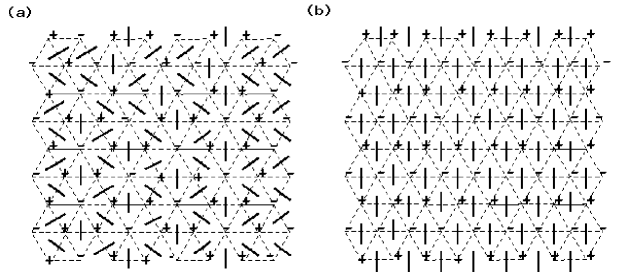
FIG. 1.: A dimer covering corresponding to a spin configuration can be obtained by putting dimers crossing the ferromagnetic bond connecting the centers of the two triangles sharing this bond. (a)the dimer covering for a random TIAFM ground state configuration (b) A special dimer covering which is mapped from the striped-order spin configuration and characterized by all vertical dimers. This dimer covering serves as a reference in defining the string picture.

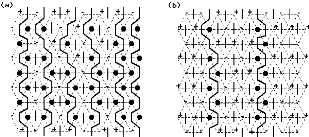
FIG. 2.: A string picture is obtained by overlapping a dimer covering with the reference dimer covering Fig.1b. The filled circles are free spins, the spins which have 3 satisfied and 3 unsatisfied bonds. As can be seen, the free spins are always tied to the strings. (a) the string mapping from the spin configuration Fig.1a (b) a string mapping which has a fewer number of strings.

FIG. 3.: (a) Entropy as a function of the string density from the work of Dhar e͡t al. [33] (b)The dimensionless free energy $f(p)$ for $\mu=0.18$. $T^{*}$ for this value of $\mu$ is 0.397. Temperature is measured in units of $1/k_{B}$.

FIG. 4.: Auto-correlation functions of string density at different temperatures. The curves have been fitted to exponentials $\exp(-\frac{t}{\tau})$.

FIG. 5.: String density correlation time $\tau$, extracted from the fitting in Fig. 4, shown as a function of temperature. Fits to a Vogel-fulcher law (solid line) and a power law (dashed line) are also shown.

FIG. 6.: Defect number auto-correlation functions and correlation times at different temperatures. (a) The auto-correlation functions can be fitted to stretched exponentials $\exp(-\frac{t}{{\tau}_{d}})^{\beta}$. The stretching exponent $\beta$ decrease with $T$ and (b) ${\tau}_{d}$ increases with $T$ in an Arrhenius fashion.

FIG. 7.: The energy auto-correlation functions, $C_{E}(t_{w},t)$, at different temperatures above $T_{g}$(top panel) and at different waiting times at a temperature $T=0.45$ which is below $T_{g}$ (bottom panel). In the top panel, the solid lines are the stretched exponential fits. The different curves at $T=0.45$ are obtained from the measurement of $C_{E}(t)$ over different ranges of $t_{w}$. From bottom to top, these ranges are $0<t_{0}<25000,18000<t_{0}<48000$ and $50000<t_{0}<80000$.

FIG. 8.: Spin auto-correlation functions at different temperatures above $T_{g}$. The curves have been fitted to power law decays with an exponential cutoff, $t^{\alpha}\exp(-\frac{t}{{\tau}_{s}})$.

FIG. 9.: The distribution functions of the string density deviation at various time differences $t$. The distribution is generated by choosing different time origins $t_{0}$. The areas under the curves have been normalized to unity. At T=0.55, a prominent non-Gaussian behavior of the distribution function is seen at $t=4000$, after which the distribution narrows back down to Gaussian. At T=0.47, the distribution becomes broader and broader with $t$, and the stationary distribution is not observed for times as long as 30,000.

FIG. 10.: The distribution functions of the magnetization deviation at various time difference $t$ measured in a square lattice Ising ferromagnet with system size $L=64$. The critical temperature $T_{c}(L)\simeq 2.27$. The areas under the curves have been normalized to unity. The relaxation behavior of the order parameter at the ferromagnetic critical point is seen to be different from that of the strings in CTIAFM.

FIG. 11.: Spin auto-correlation functions for different string density sectors, $p$. For $p\geq 0.25$, the relaxation can be described by a power law. For $p\leq 0.25$, the relaxation is best fit to a stretched exponential form.

FIG. 12.: The top panel shows the overlap, $Q(t_{w},t)$, versus the correlation function $C(t_{w},t)$. In the bottom panel $C(t_{w},t)$ and $Q(t_{w},t)$ are shown for different ranges of $t_{w}$.

FIG. 13.: (a)Time history of the string density after the CTIAFM is quenched to $T=0.35$. At each of the different times marked by arrows in (a), three copies of the system are made and evolved with independent noise realizations. The panels (b),(c) and (d) depict the history of string density of the three copies made at $t_{w}=2000,40000,$ and $76000$, respectively.

FIG. 14.: $Q(t_{w},t)$ and $C(t_{w},t)$ after quenching triangular ferromagnet to just above $T_{c}$. From the top panel, $Q(t_{w},t)$ is seen to reach a finite value for $t_{w}=50$ and vanish for $t_{w}=1000$ and $12000$ as $C(t_{w},t)$ decays to zero. In bottom three panels $Q(t_{w},t)$ and $C(t_{w},t)$ are shown as functions of time for different $t_{w}$. The behavior of $Q(t_{w},t)$ at small $t_{w}$ when the system is yet to reach equilibrium is seen to be different from that of the CTIAFM in the glass phase.

FIG. 15.: The temperature dependence of the energy $E$ for different cooling rates $\gamma$.

FIG. 16.: Defect density $\rho(t)$ as a function of $\beta=T^{-1}$ for different cooling rates, $\gamma$, compared to the equilibrium, Arrhenius form.

TABLE I.: Results from fitting the string auto-correlation functions and defect number auto-correlation functions. The first column is the temperature. The second and third are the correlation time of the string density and its associated error bars from the exponential fit. The next two columns are the values of $\beta$ and ${\tau}_{d}$ from the defect number auto-correlation functions fitted to a stretched exponential form. The last two columns are the values of ${\tau}_{E}$ and $\beta$ from the energy auto-correlation fitted to a stretched exponential form.

$T$	$\tau\ (string)$	$\Delta$$\tau$ (string)		$\beta\ (defect)$	$\tau_{d}\ (defect)$		$\tau_{E}\ (Energy)$	$\beta\ (Energy)$
0.6	457	45		0.44 $\pm$ 0.01	13.5		12.6	0.42 $\pm$ 0.004
0.57	1223	119		0.39 $\pm$ 0.01	15.3		13.4	0.38 $\pm$ 0.01
0.55	2161	505		0.38 $\pm$ 0.01	19.8		23.0	0.40 $\pm$ 0.04
0.52	2860	593		0.36 $\pm$ 0.02	23.8		29.8	0.38 $\pm$ 0.02
0.50	4124	378		0.37 $\pm$ 0.02	33.0		49.0	0.35 $\pm$ 0.01
0.48	7081	370		0.34 $\pm$ 0.02	45.8		67.9	0.34 $\pm$ 0.03
0.47	15472	2575		0.33 $\pm$ 0.01	54.5		87.2	0.32 $\pm$ 0.03

TABLE II.: The correlation time $\tau_{s}$ and exponent $\alpha$ extracted from the fitting of the spin auto-correlation function to the form $C\ t^{-\alpha}\exp(-\frac{t}{{\tau}_{s}})$ at different temperatures.

$T$	${\tau}_{s}\ (spin)$	$\alpha\ (spin)$	C (prefactor)
0.6	865	0.36	0.88
0.55	1140	0.32	0.78
0.52	1980	0.30	0.75
0.50	2170	0.28	0.72
0.47	4910	0.25	0.64

TABLE III.: Results obtained from fitting the spin auto-correlation functions in different string-density sectors to the stretched exponential form $\exp{(-(t/\tau_{s})^{\beta})}$

. $string\ density$ ${\tau}_{s}\ (spin)$ $\beta\ (spin)$ p=0.042 $1.9\times 10^{5}$ 0.28 p=0.083 7435 0.32 p=0.125 1522 0.33

REFERENCES

- [1] C. A. Angell, J. Phys. Chem. 49, 863 (1988), M. D. Ediger, C. A. Angell, and S. R. Nagel, J. Phys. Chem. 100, 13200 (1996) W. Götze and L. Sjogren, Rep. Prog. Phys. B 55, 241 (1992)
- [2] M. T. Cicerone and M. D. Ediger, J. Chem. Phys 103, 5684 (1995) and references therein.
- [3] M. Mezard, G. Parisi and M. A. Virasoro, Spin Glass Theory and Beyond, (World Scientific, Singapore, 1987).
- [4] H. Yin and B. Chakraborty, Phys. Rev. Lett. 86, 2058 (2001).
- [5] C. A. Angell, Science 267, 1924 (1995)
- [6] N. Goldenfeld, Lectures on Phase Transitions and the Renormalization Group,(Addison-Wesley, New York, 1992)
- [7] E. R. Weeks, J. C. Crocker, A. C. Levitt, A. Schofield, D. A. Weitz, Science 287, 627 (2000);W. K. Kegel, A. van Blaaderen, Science 287, 290 (2000).
- [8] E. Vidal Russel and N. E. Israeloff, Nature 408, 695 (2000)
- [9] C. Donati, J. F. Douglas, W. Kob, S. J. Plimpton, P. H. Poole and S. C. Glotzer, Phys. Rev. Lett. 80, 2338 (1998); W. Kob, C. Donati, S. J. Plimpton, P. H. Poole, and S. C. Glotzer, Phys. Rev. Lett. 79, 2827 (1997); C. Donati, S. C. Glotzer, P. H. Poole, W. Kob, and S. J. Plimpton,Phys. Rev. E 60, 3107 (1999).
- [10] G. Adam and J. H. Gibbs, J. Chem. Phys. 43, 139 (1965), J. H. Gibbs and E. A. DiMarzio, J. Chem. Phys. 28, 373 (1958).
- [11] M. Mezard and G. Parisi, preprint cond-mat/0002128, and references therein.
- [12] W. Kauzman, Chem. Rev. 43, 219 (1948)
- [13] R. Richert and C. A. Angell, J. Chem. Phys. 108, 9016 (1998).
- [14] D. J. Gross and M. Mezard, Nucl. Phys. B240, 431 (1984)
- [15] T. R. Kirkpatrick and P. G. Wolynes, Phys. Rev. A 34, 1045 (1986), Phys. Rev. A 35, 3072 (1987), T. R. Kirkpatrick and D. Thirumalai, Phys. Rev. Lett. 58, 2091 (1987), Phys. Rev. B 36, 5388 (1987), T. R. Kirpatrick, D. Thirumalai, and P. G. Wolynes, Phys. Rev. A 40, 1045 (1989)
- [16] J. P. Bouchaud and M. Mezard, J. Phys. I 4, 1109 (1994).
- [17] X. Xia, and P. G. Wolynes, preprint cond-mat/0008432
- [18] S. Sastry, P. G. Debenedetti and F. H. Stillinger, Nature 393, 554 (1998).
- [19] S. Sastry, preprint cond-mat/0101079.
- [20] J. P. Sethna, J. D. Shore and M. Huang, Phys. Rev. B 44, 4943 (1991)
- [21] D. S. Fisher, Phys. Rev. Lett. 56, 416 (1986).
- [22] A. Lipowski, J. Phys. A 30, 7365 (1997), A. Lipowski and D. A. Johnston, Phys. Rev. E 61, 6375 (2000), A. Lipowski, D. A. Johnston, and D. Espriu, Phys. Rev. E 62, 3404 (2000)
- [23] M. R. Swift, H. Bokil, R. D. M. Travasso, and A. J. Bray, preprint cond-Mat/0003384
- [24] J. D. Shore and J. P. Sethna, Phys. Rev. B 43, 3782 (1991), J. D. Shore, M. Holzer, and J. P. Sethna, Phys. Rev. B 46, 11376 (1992)
- [25] M. E. J. Newman, and C. Moore, Phys. Rev. E 60, 5068 (1999), J. P. Garrahan and M. E. J. Newman,Phys. Rev. E 62, 7670 (2000)
- [26] Lei Gu, Bulbul Chakraborty, P. L. Garrido, Mohan Phani and J. L. Lebowitz, Phys. Rev. B 53, 11985 (1996).
- [27] G. H. Wannier, Phys. Rev. 79, 357 (1950)
- [28] R. M. F. Houtappel, Physica 16, 425 (1950)
- [29] J. Stephenson, J. Math Phys. A 11, 413 (1970).
- [30] Henk W. J. Blöte and M. Peter Nightingale, Phys. Rev. B 47, 15046 (1993) and references therein.
- [31] C. Zeng and C. L. Henley, Phys. Rev. B 55, 14935 (1997)
- [32] H. W. J. Blöte, H. J. Hilhorst, J. Phys. A: Math. Gen. 15, L631 (1982).
- [33] A. Dhar, P. Choudhuri and C. Dasgupta, Phys. Rev. B 61, 6227 (2000).
- [34] Z. Y. Chen and M. Kardar, J. Phys. C 19, 6825 (1986)
- [35] Lei Gu and Bulbul Chakraborty, Mat. Res. Soc. Symp. Proc 455, 229 (1997), and cond-mat/9612103; Lei Gu, Ph. D. Thesis, Brandeis University, 1999.
- [36] C. Zeng, P. L. Leath and T. Hwa, Phys. Rev. Lett. 83, 4860 (1999).
- [37] J. Kondev, Phys. Rev. Lett. 78, 4320 (1997); J.L. Jacobsen and J. Kondev, Nucl. Phys. , 635 (1998).
- [38] B. Chakraborty, L. Gu and H. Yin, J. Phys. Condens. Mat. 12, 6487 (2000)
- [39] W. Klein and C. Unger, Phys. Rev. B 28, 445 (1983).
- [40] Hui Yin, Ph.D thesis, Brandeis University, 2001.
- [41] P. Jund, R. Jullien and I. Campbell, preprint cond-mat/0011494
- [42] H. Vogel, Phys. Z. 22, 645 (1921), G. S. Fulcher, J. Am. Ceram. Soc. 8, 339 (1925)
- [43] A. Barrat, R. Burioni, and M. Mezard, J. Phys. A 29, 1311 (1995)
- [44] It can be shown that for systems in equilibrium, , the overlap between two copies evolving independently for time , is equal to [43].