The multi-fractal structure of contrast changes in natural images: from sharp edges to textures.

Abstract

We present a formalism that leads very naturally to a hierarchical description of the different contrast structures in images, providing precise definitions of sharp edges and other texture components. Within this formalism, we achieve a decomposition of pixels of the image in sets, the fractal components of the image, such that each set only contains points characterized by a fixed stregth of the singularity of the contrast gradient in its neighborhood. A crucial role in this description of images is played by the behavior of contrast differences under changes in scale. Contrary to naive scaling ideas where the image is thought to have uniform transformation properties (?), each of these fractal components has its own transformation law and scaling exponents. A conjecture on their biological relevance is also given.

Neural Computation 12, 763-793 (2000)

1 Introduction

It has been frequently remarked that natural images contain redundant information. Two nearby points in a given image are very likely to have very similar values of light intensity, except when an edge lies between them. In this case, the sharp change in luminosity also represents a loss of predictability, because probably the two points belong to two different objects, with almost independent luminosities. Since they cannot be predicted easily, it is frequently said that edges are the most informative structures in the image and that they represent their independent features (?). Anyone´s subjective experience is consistent with this: most people would start drawing a scene by tracing the lines of the obvious contours in the scene. Even more, the picture can be understood by anyone observing that sketch. Only afterwards, one starts adding texture to the light-flat areas in the drawing. These textures represent the less informative data about the position and intensity of the light sources. It seems that different structures can be distinguished in every image, following a hierarchy defined according to their information content, from the sharpest edges to the softest textures.

Image processing techniques also emphasize the fact that edges are the most prominent structures in a scene. A large variety of methods for edge detection have been proposed, e.g. high pass filtering, zero-crossing, wavelet projections, … (?). But once the edges have been extracted from the image, these methods do not address the problem of how to describe and obtain the other structures. In order to detect these other sets and to extract them in the context of an organized hierarchy, it is necessary to provide a more general mathematical framework and, in particular, to define the variables suitable to perform this classification.

In this paper we present a more rigorous approach to these issues, proposing precise definitions of edges and other texture components of images. As we shall see, our formalism leads very naturally to a hierarchical description of the different structures in the images, achieving a decomposition of its pixels in sets, or components, ranging from the most to the less informative structures.

Another motivation to understand the role played by edges in natural images is related to the development of the early visual system. The brain has to solve the problem of how to represent and transmit efficiently the information it receives from the outside world. As it has been frequently pointed out (?, ?, ?, ?), cells located in the first stages of the visual pathway do this by trying to take advantage of statistical regularities in the image ensemble. The idea is that since natural images are highly redundant over space, they have to be represented in a compact and non-redundant way before being transmitted to inner areas in the brain. In order to do this, it is first necessary to know the regularities of the images, which then could be used to build more appropriate and efficient internal representations of the environment.

The statistical properties of natural images have been studied for many years, but the effort was mainly restricted to the second order statistics. The emphasis was put on the two-point correlation first because of the simplicity of the analysis, and secondly because its Fourier transform (i.e. the power spectrum) has a power law behavior that reflects the existence of scale invariant properties in natural images. This implies that the second order statistics does capture some of the regularities. However most of the underlying statistical structure remains unveiled. One can easily convince oneself that most of the correlations in the image are still present after whitening is performed: the contours of the objects in the whitened image are still easily recognizable (?). The conclusion is that non-gaussian statistical properties of edges are important to describe natural images, a fact that has also been recognized by (?, ?). However, no systematic studies of the statistical properties of edges had been done until very recently (?).

A complete characterization of the regularities of natural images is impossible, and probably useless. Some intuition is necessary to guide the search for regularities. The aim of this work is to exploit the basic idea that changes in contrast are relevant because they occur at the most informative pixels of the scene. Hence we focus our attention in the statistics of changes in luminosity. Since these changes are graded, the task could seem rather difficult and even hopeless, but the solution to this problem turns out to be quite simple and elegant. A single parameter is enough to describe a full hierarchy of differences in contrast and the hierarchy can be explicitly constructed. Moreover, it is intimately related to the scale invariance properties of the image, which are certainly more elaborated than those that have been used until now but are still simple enough and have plenty of structure to be detected by a network adapting to the statistics of the stimuli.

To understand these scale invariances we need first the basic concepts of multiscaling and multifractality (?), together with a simple explanation of their meaning for images. While in naive scaling there is a single transformation law throughout the image (which is then said to be a fractal), in the more general case there is no invariance under a global scale transformation but the space can be decomposed in sets with a different transformation law for each of them (the image is then said to be a multifractal).

To make this concept more precise, let us consider a simple situation where a set of images present a single type of changes in contrast: the luminosity suddenly changes from one (roughly) constant value to another. In this case, a natural description of the properties of changes in contrast would be to count the number of such changes that appear along a segment of size $r$, oriented in a given direction. The statistical distribution of the position and size of these jumps in contrast would give relevant information about an ensemble of such images. However, in real images this counting is not enough to describe well the properties of contrast changes. This is because these changes do not follow such a simple pattern: some of them can be sharp (the notion of sharp changes has to be given), but there will also be all types of softer textures that would be lost by just counting the most noticeable changes. It is then necessary to consider all of them as a whole. A natural way to deal with contrast changes is by defining a quantity that accumulates all of them, whatever their strength, contained inside a scale $r$, that is:

$$\epsilon_{r}(\vec{x})\>=\>\frac{1}{r^{2}}\int_{x_{1}-\frac{r}{2}}^{x_{1}+\frac{r}{2}}dx_{1}^{\prime}\int_{x_{2}-\frac{r}{2}}^{x_{2}+\frac{r}{2}}dx_{2}^{\prime}\;\;\mid\nabla C({\vec{x}^{\prime}})\mid\;\;.$$ (1)

Hereafter, the contrast $C(\vec{x})$ is taken as $C(\vec{x})=I(\vec{x})-\langle I\rangle$, where $I(\vec{x})$ is the field of luminosities and $\langle I\rangle$ its average value across the ensemble. The bidimensional integral on the right hand side, defined on the set of pixels contained in a square of linear size $r$, is a measure of that square . It is divided by the factor $r^{2}$, which is the usual Lebesgue measure (which we will denote $\lambda$) of a square of linear size $r$. The quantity $\epsilon_{r}(\vec{x})$ can then be regarded as the ratio between these two measures. More generally, we can define the measure $\mu$ of a subset $A$ of image pixels as

$$\mu(A)\>=\>\int_{A}d\vec{x}^{\prime}\;\mid\nabla C(\vec{x}^{\prime})\mid\;\;,$$ (2)

($\int_{A}d\vec{x}^{\prime}$ means bidimensional integration over the set $A$) what we will call the Edge Measure (EM) of the subset $A$. It is also possible to generalize the definition of $\epsilon_{r}$ for any subset $A$:

$$\epsilon_{A}\>=\>\frac{\mu(A)}{\lambda(A)}\hskip 28.45274pt.$$ (3)

$\epsilon_{A}$ is a density, a quantity that compares how much the distribution of $|\nabla C|$ deviates from being homogeneously distributed on $A$. We shall call it the Edge Content (EC) of the set $A$. Denoting $B_{r}(\vec{x})$ the “ball” of radius $r$ centered around $\vec{x}$, it is clear that $\epsilon_{r}(\vec{x})\equiv\epsilon_{B_{r}(\vec{x})}$, so this definition generalizes the previous one. We shall refer to $\epsilon_{r}(\vec{x})$ as the Edge Content of $\vec{x}$ at the scale $r$. Notice that $\epsilon_{dr}(\vec{x})$ is the $\mu$-density at $\vec{x}$, $|\nabla C|(\vec{x})$. Thus, eq. (2) can be symbolically expressed as

$$d\mu(\vec{x})=|\nabla C|(\vec{x})d\vec{x}\;\;.$$ (4)

The main point is that contrast changes are distributed over the image in such a way that the Edge Content has rather large contributions even from pixels that are very close together. As a consequence, the measure presents a rather irregular behavior. But it is precisely in its irregularity where the information about the contrast lies. Let us assume for instance that, as $r$ becomes very small, the measure behaves at every point $\vec{x}$ as

$$\mu\left(B_{r}(\vec{x})\right)\>\equiv\>\mu_{r}(\vec{x})\>=\>\alpha(\vec{x})\;r^{h(\vec{x})+d}\;\;,$$ (5)

where $d=2$ is the dimension of the images. For convience a shift in the definition of the exponent of $\mu_{r}(\vec{x})$ has been introduced. The Edge Content then verifies :

$$\epsilon_{r}(\vec{x})\>=\>\alpha(\vec{x})\;r^{h(\vec{x})}\;\;,$$ (6)

and this choice of $h(\vec{x})$ removes trivial dependencies on $r$. The exponent $h(\vec{x})$ is just the singularity exponent of $|\nabla C|(\vec{x})$. That is, $h<0$ indicates a divergence of $|\nabla C|(\vec{x})$ to infinity, while $h>0$ indicates finiteness and continuous behavior. The greater the exponent the smoother is the density around that point. In general, we will talk about “singularity” even for the positive $h$ cases.

Thus, the meaning of eq. (5) is that all the points are singular (in this wide sense), and that the singularity exponent is not uniform. This irregular behavior would allow us to classify the pixels in a given image: the set of pixels with a singularity exponent contained in the interval $[h-\Delta_{h},h+\Delta_{h}]$ (where $\Delta_{h}$ is a small positive number) define a class $F_{h}$. These classes are the fractal components of the image. The smaller the exponent the more singular is the class, and the most singular component is the one with the smallest value of $h$. A measure $\mu$ verifying eq. (5) in every point $\vec{x}$ is called a multifractal measure.

We will refer to these components of the images as fractal sets because it will be seen that they are of a very irregular nature. One way to characterize the odd arrangement of the points in fractal sets is by just counting the number of points contained inside a given ball of radius $r$; we will denote by $N_{r}(h,\Delta_{h})$ this number for the set $F_{h}$. As $r\rightarrow 0$ it is verified that

$$N_{r}(h,\Delta_{h})\>\sim\>r^{D(h)}.$$ (7)

This new exponent, $D(h)$, quantifies the size of the set of pixels with singularity $h$ as the image is covered with small balls of radius $r$. It is the fractal dimension of the associated fractal component $F_{h}$, and the function $D(h)$ is called the dimension spectrum (or the singularity spectrum) of the multifractal. It is also worth estimating the probability for a ball of radius $r$ to contain a pixel belonging to a given fractal component. Its behavior for small scales $r$ is:

$$Prob(h,\Delta h)\>\sim\>r^{d-D(h)}\;\;,$$ (8)

where $d=2$ as before. Notice that, since $r$ is small, this quantity increases as $D(h)$ approaches $d$.

The multifractal behavior also implies a multiscaling effect: as every fractal component possesses its own fractal dimension, each of them changes differently under changes in the scale. Thus, although every component has no definite scale and is invariant under the scale transformations, scale invariance is broken for a given image: the points in the image transform with different exponents, according to the fractal component to which they belong. This leads to the presence of intermittency effects: if the image were enlarged, its statistical properties would change. Self-similarity is lost. However, scale invariance is restored in the averages over an ensemble of such images.

At this point one may wonder if a multifractal behavior is actually realized in natural images. One way to check its validity is to verify that eq. (5) is indeed correct. This in turn leads us to the technical problem of how to obtain in practice the exponent $h(\vec{x})$ at a given pixel $\vec{x}$ of the image. This is a local analysis where the singularity is found by looking at the neighbourhood of the point $\vec{x}$. It has the advantage that it not only provides us with a tool to check the multifractal character of the measure but it also gives a way to decompose each image in its fractal components. These issues are addressed in the next Section. The multifractality of the measure can also be studied by means of statistical methods. In this case one looks for the effect of the singulaties on the moments of marginal distributions of, e.g., the Edge Content defined in eq. (1). This is done in Section 3, where the important notions of self-similarity, extended self-similarity and multiplicative processes are explained. Once the relevant mathematical tools are given, these are used in Section 4 to analyze natural images. First in subsection 4.2 we check that the measure introduced in eq. (2) is indeed multifractal. Examples of fractal components of natural images are also presented in the same section. After this we study the consistency between the singularity analysis and the statistical analysis of the measure (subsection 4.3). The results of the numerical study of self-similarity properties of the contrast $C(\vec{x})$ and of the measure density $|\nabla C|(\vec{x})$ are presented in subsection 4.4. The discussion of the results and perspectives for future work are given in the last section. Some technical aspects are included in the Appendix.

2 Singularity analysis: The wavelet transform

In this section we present the appropriate techniques to deal with multifractal measures, and especially with those adapted to natural images. To check if $\mu$ defines a multifractal measure and to obtain the local exponent $h(\vec{x})$, we need to analyze the dependence of $\mu(B_{r}(\vec{x}))$ on the scale $r$. Unfortunately, direct logarithmic regression performed on eq. (5) yields rather coarse results when it is applied on discretized images, allowing only the detection of very sharp, well isolated features. It is then necessary to use more sophisticated methods. A convenient technique for this purpose (?, ?, ?) is the wavelet transform (see e.g. (?)). Roughly speaking, the wavelet transform provides a way to interpolate the behavior of the measure $\mu$ over balls of radius $r$ when $r$ is a non-integer number of pixels. Besides, if the image is a discretization of a continuous signal, the wavelet analysis is the appropriate technique to retrieve the correct exponents, as it is explained later on.

The wavelet transform of a measure $\mu$ is a function that is not localized, neither in space nor in frequency. Its arguments are then the site $\vec{x}$ and the scale $r$. It also involves an appropriate, smooth interpolating function $\Psi(\vec{x})$. More precisely, the wavelet transform of $\mu$ is:

$$T^{r}_{\Psi}d\mu(\vec{x})\;\equiv\;\int d\mu(\vec{x}^{\prime})\>\Psi_{r}(\vec{x}-\vec{x}^{\prime})\;=\;\frac{d\mu}{d\vec{x}}\otimes\Psi_{r}(\vec{x})\;\;,$$ (9)

where $\Psi_{r}(\vec{x})\equiv\frac{1}{r^{d}}\Psi(\frac{\vec{x}}{r})$. The important point here is that for the case of a positive measure it can be proved that:

$$T^{r}_{\Psi}d\mu(\vec{x}_{0})\sim r^{h(\vec{x}_{0})}$$ (10)

if and only if $\mu$ verifies eq.(5) ($h$ being exactly the same) and $\Psi$ decreases fast enough (see (?) and references therein). In that way, this property allows us to extract the singularities directly from $T^{r}_{\Psi}d\mu$. It is very important to remark that $\Psi$ can be a positive function, what makes an essential difference with respect to the analysis of multiaffine functions (see section 3.4).

In general the ideal, continuous measure $d\mu(\vec{x})$ is unknown. In these cases the data is given by a discretized sampling, which in our case is a collection of pixels. One can reasonably argue that the pixel is the result of the convolution of an ideal signal with a compact support function $\chi_{a}(\vec{x})$ (describing, e.g., the resolution $\sim a$ of the optical device). In this case, under convenient hypothesis, the wavelet transform yields the correct projection of the ideal signal. Let us call $\vec{x}_{(n_{1},n_{2})}\equiv\vec{x}_{\vec{n}}$ the positions of the pixels in the discretized sample and $C_{\vec{n}}$ the values of the discretized version of the contrast; then

$$C_{\vec{n}}\;=\;T^{a}_{\chi}C(\vec{x}_{n})\,\equiv\,C\otimes\chi_{a}(\vec{x}_{\vec{n}})\;,$$ (11)

Taking the sample $\{\vec{x}_{\vec{n}}\}$ in such a way that the centers of adjacent pixels are at a distance larger than $a$, it is verified that:

$$\nabla C_{\vec{n}}\;\equiv\;\left(C_{(n_{1}+1,n_{2})}-C_{(n_{1},n2)}\>,\>C_{(n_{1},n_{2}+1)}-C_{(n_{1},n2)}\right)\;\sim\;\nabla C\otimes\chi_{a}(\vec{x}_{\vec{n}})$$ (12)

and so the discretized version $\mu^{(dis)}$ of the ideal measure $\mu$, can be considered as a wavelet coefficient of the continuous $\mu$ with the wavelet $\chi$ at the scale $a$, namely

$$d\mu^{(dis)}_{\vec{n}}\sim d\vec{x}\;\;|\nabla C|\otimes\chi_{a}(\vec{x}_{\vec{n}})\;=\;d\vec{x}\;\;T^{a}_{\chi}d\mu(\vec{x}_{\vec{n}})\;\;.$$ (13)

Taking into account that the convolution is associative, the discretized wavelet analysis of $d\mu_{\vec{n}}^{(dis)}$ with a wavelet $\Psi$ can be simply expressed as:

$$T^{r}_{\Psi}d\mu^{(dis)}(\vec{x}_{\vec{n}})\sim T^{r}_{\Psi\otimes\chi_{\frac{a}{r}}}d\mu(\vec{x}_{\vec{n}})$$ (14)

that is, analyzing the discretized measure $\mu^{(dis)}$ with a wavelet $\Psi$ is equivalent to analyze the continuous measure $\mu$ with a wavelet $\Psi\otimes\chi_{\frac{a}{r}}$. But if the scale $r$ is large enough compared to the photoreceptor extent $a$, $\chi_{\frac{a}{r}}(\vec{x})\sim\delta(\vec{x})$, which does not depend on $r$. Thus, if the internal size $a$ is small enough to allow fine detection, we can recover the correct exponent at the point $\vec{x}_{\vec{n}}$ by just analyzing the discretized measure. Conversely, the extent $a$ imposes a lower cut-off in the details that can be observed in any image constructed by pixels: as it is just the size of the pixel, the estimation of the singularity exponent at a given point requires to perform the analysis over scales containing several pixels.

This analysis is similar to that performed in (?, ?): any image is analyzed by means of its scaling properties under wavelet projection. There are however important differences between the study performed by these authors and the present work. The first difference concerns the basic scalar field to be analyzed: Mallat and Zhong considered $C(\vec{x})$ instead of $|\nabla C|(\vec{x})$, which we prefer because, as it will be shown later on, it is the $\mu$-density of a multifractal measure $\mu$ (see Section 4). Another difference is methodological: in this paper we intend to classify the points according its singularity exponent to form every fractal component, while the previous papers were devoted to obtain only the wavelet transform modulus maxima, a concept related but different from what we will call the most singular component, that is, only one (although the most important) of the fractal components. The third difference concerns motivation: we want to classify every point with respect to a hierarchical scheme, while these authors search a wavelet-based optimal codification algorithm, in the sense of providing an (almost) perfect reconstruction algorithm from the wavelet maxima.

3 Statistical self-similarity of natural images

In this section we introduce the basic concepts of the statistical approach, defining at the same time new variables which are closer to the wavelet analysis.

3.1 SS and ESS

From the statistical point of view, $\mu_{r}$ is a random variable, in the sense that given a random point $\vec{x}$ in an arbitrary image $\cal{I}$ the value of $\mu^{\cal{I}}_{r}(\vec{x})$ cannot be deterministically predicted.

By definition, the multifractal structure is a multiscaling effect. This multiscaling should be somehow apparent from the dependence of the probability density of $\mu_{r}$ on the scale parameter $r$. To determine the whole probability density function of $\mu_{r}$ requires a large dataset, especially for the rare events; besides its dependence on $r$ could mix multiscaling effects in a complicated way. On the contrary, the $p$-moments of $\mu_{r}$ (that is, the expectation values of $\mu_{r}$ raised to the $p$-th power) suffice to characterize completely the probability density, and given that they are averages of powers of $\mu_{r}$ they are likely to depend on $r$ in a simple way, somehow related to the behavior of the measure in eq. (5).

It is more convenient to deal with the $p$-moments of normalized versions of $\mu_{r}$ such as the Edge Content $\epsilon_{r}\equiv\frac{1}{r^{2}}\mu_{r}$ or the wavelet projections $|T^{r}_{\Psi}d\mu|$. They are normalized in such a way that the first order moments, $\langle\epsilon_{r}\rangle$ and $\langle|T^{r}_{\Psi}d\mu|\rangle$, do not depend on $r$: the trivial factor $r^{pd}$ is hence removed from the random variable.

As we will see later on, the moments $\langle\epsilon_{r}^{p}\rangle$ and $\langle|T^{r}_{\Psi}d\mu|^{p}\rangle$ exhibit the remarkable scaling properties of Self-Similarity (SS):

$$\langle\epsilon_{r}^{p}\rangle\;=\;\alpha_{p}\>r^{\tau_{p}}$$ (15)

(analogously for $|T^{r}_{\Psi}d\mu|$ with exponents $\tau_{p}^{\Psi}$) and of Extended Self-Similarity (ESS) (referred to the moment of order $2$) (?, ?, ?):

$$\langle\epsilon_{r}^{p}\rangle\;=\;A(p,2)\left[\langle\epsilon_{r}^{2}\rangle\right]^{\rho(p,2)}\;\;,$$ (16)

(and similarly for $|T^{r}_{\Psi}d\mu|$ with exponents $\rho^{\Psi}(p,2)$). ESS has been referred to the moment of order $2$, but eq (16) trivially implies that any moment can be expressed as a power of the moment of order $q$ with an exponent $\rho(p,q)=\frac{\rho(p,2)}{\rho(q,2)}$.

In this way, we have the sets of SS exponents $\tau_{p}$ and ESS exponents $\rho(p,2)$ for $\epsilon_{r}$ and similarly the exponents $\tau_{p}^{\Psi}$ and $\rho^{\Psi}(p,2)$ for $T^{r}_{\Psi}d\mu$. Notice that if SS holds also does ESS, in which case there is a simple relation between $\tau_{p}$ and $\rho(p,2)$:

$$\tau_{p}\;=\;\tau_{2}\>\rho(p,2)\;\;.$$ (17)

The actual dependence of $\tau_{p}$ and $\rho(p,2)$ on $p$ determines the fractal structure of the system. A trivial dependence $\tau_{p}\propto p$ would reveal a monofractal structure. A different dependence on $p$ indicates the existence of a more complicated (multifractal) geometrical structure.

3.2 The multiplicative process

A random variable subtending an area of linear size $r$ and which possesses SS (eq. (15)) and ESS (eq. (16)) can be described statistically by means of a multiplicative process (?, ?). The statistical formulation is rather simple: given two different scales $r$ and $L$ such that $r<L$, there is a simple stochastic relation between the Edge Contents at these two scales :

$$\epsilon_{r}\;\doteq\;\alpha_{rL}\>\epsilon_{L}$$ (18)

where $\alpha_{rL}$ is a random variable, independent of the Edge Content, which describes how the change between these two scales takes place. The symbol “$\doteq$” indicates that both sides of the equation are distributed in the same way, but this does not necessarily imply the validity of the relation at every pixel of a given image. The random variables $\alpha_{rL}$ between all possible pairs of scales $r$ and $L$ are said to define a multiplicative process.

Let us understand in a more intuitive way the meaning of this process. It is rather clear that given the distribution of $\epsilon_{L}$ at a fixed large scale $L$, to compute the distribution of the Edge Content $\epsilon_{r}$ it is enough to know the distribution of $\alpha_{rL}$. But let us now introduce an intermediate scale $r^{\prime}$. One could also obtain first $\epsilon_{r^{\prime}}$ using $\alpha_{r^{\prime}L}$ and then $\epsilon_{r}$ by means of $\alpha_{rr^{\prime}}$. Thus, the multiplicative process must verify the cascade relation:

$$\alpha_{rL}\;=\;\alpha_{rr^{\prime}}\>\alpha_{r^{\prime}L}\;\;,$$ (19)

that tells us that the variables $\alpha_{rL}$ are infinitely divisible. Infinitely divisible stochastic variables are then completely characterized by their behavior under infinitely small changes in the scale, that is, by $\alpha_{r,r+dr}$. The simplest example of an infinitely divisible random variable $\alpha_{rL}$ is the one having a binomial infinitesimal distribution, namely:

$$\alpha_{r,r+dr}\;=\;\left\{\begin{array}[]{ccc}\\ 1-\Delta\frac{dr}{r}&,&\mbox{with probability $1-[d-D_{\infty}]\frac{dr}{r}$}\\ \\ \beta(1-\Delta\frac{dr}{r})&,&\mbox{with probability $[d-D_{\infty}]\frac{dr}{r}$}\\ \\ \end{array}\right.$$ (20)

The form of this process is determined by its compatibility with eq. (19); see for instance (?, ?, ?) for a detailed study. Moreover, there are only two free parameters: it is verified that $d-D_{\infty}=\Delta/(1-\beta)$. They have also to satisfy the following bounds: $0<\beta<1$ and $0<\Delta<1$.

The infinitesimal process (20) can be easily interpreted in terms of the Edge Content and the measure density:

• Probability $\;=1-[d-D_{\infty}]\frac{dr}{r}$ : this is the most likely situation. In this case the Edge Content (and consequently the measure) changes smoothly under small changes in scale: $\alpha_{r,r+dr}$ is close to one and its variation is proportional to $d\ln r$.

• Probability $\;=[d-D_{\infty}]\frac{dr}{r}$ : in this unlikely case, under infinitesimal changes in scale the Edge Content undergoes finite variations, which is reflected in the fact that $\alpha_{r,r+dr}$ deviates from one by a factor $\beta$. The $\mu$-density $|\nabla C|$ must then be divergent somewhere along the boundary of the ball of radius $r$, and the parameter $\beta$ is a measure of how sharp this divergence is.

The process for non-infinitesimal changes in scale can be easily derived from the infinitesimal process presented in eq (20). In this case the random variable $\alpha_{rL}$ follows a Log-Poisson process (?); its probability distribution $\rho_{\alpha_{rL}}(\alpha_{rL})$ has the form:

$$\rho_{\alpha_{rL}}(\alpha_{rL})\;=\;\left[\frac{r}{L}\right]^{d-D_{\infty}}\>\sum_{n=0}^{\infty}\frac{(d-D_{\infty})^{n}}{n!}\>\left[\ln\frac{L}{r}\right]^{n}\>\delta(\alpha_{rL}-\beta^{n}\>\left(\frac{r}{L}\right)^{-\Delta})$$ (21)

If a multiplicative process is realised the Edge Content has the SS and the ESS properties, eqs. (15) and (16). Thus, knowledge of the ESS exponents $\rho(p,2)$ and of $\tau_{2}$ is enough to compute $\tau_{p}$ using eq. (17). For the Log-Poisson process the ESS exponents are:

$$\rho(p,2)\;=\;\frac{p}{1-\beta}\>-\>\frac{1-\beta^{p}}{(1-\beta)^{2}}$$ (22)

which depend only on $\beta$. This process was proposed in (?) for turbulent flows, so we will refer to it either as the She-Leveque (S-L) or as the Log-Poisson model. The SS exponents are:

$$\tau_{p}\;=\;-\Delta p\>+\>(d-D_{\infty})(1-\beta^{p})$$ (23)

which compared with eq. (17) gives the following set of relations :

$$\left\{\begin{array}[]{ccccc}\Delta&=&-\frac{\tau_{2}}{1-\beta}&&\\ d-D_{\infty}&=&-\frac{\tau_{2}}{(1-\beta)^{2}}&=&\frac{\Delta}{1-\beta}\end{array}\right.$$ (24)

This means that the model has only two free parameters, that can be chosen to be $\tau_{2}$ and $\beta$ or $\Delta$ and $D_{\infty}$, for instance. The geometrical interpretation of the last two is very interesting (?), and will be explained in the next subsection. For the time being let us notice that the maximum value of the EC, $\parallel\epsilon_{r}\parallel_{\infty}$, also follows a power law with exponent $-\Delta$,

$$\parallel\epsilon_{r}\parallel_{\infty}\;=\;\alpha_{\infty}\>r^{-\Delta}$$ (25)

and thus the parameter $\Delta$ characterizes the most divergent behavior present in natural images.

3.3 SS and multifractality

Let us now analyze in more detail the geometrical meaning of the model and its relation with the singularities described in Section 2. For a multifractal measure $\mu$ with singularity spectrum $D(h)$ there is an important relation between the SS exponents $\tau_{p}$ and $D(h)$. Let us denote by $\rho_{h}(h)$ the probability density of the distribution of the singularity exponents $h$ in the image. Then, partitioning the image pixels according to their values of $h$, eq. (6) can be expressed, for $r$ small enough, as:

$$\langle\epsilon_{r}^{p}\rangle\;\sim\;\int dh\>\rho_{h}(h)\langle\alpha^{p}\rangle_{{}_{F_{h}}}\>r^{hp+d-D(h)}\;\;.$$ (26)

The factor $r^{d-D(h)}$ comes from the probability of a randomly chosen pixel being in the fractal $F_{h}$ (see eq. (8)) and guarantees the correct normalization of $\langle\alpha^{p}\rangle_{{}_{F_{h}}}$ (see e.g. (?, ?) for details). For very small $r$ the application of the saddle point method to eq. (26) yields:

$$\langle\epsilon_{r}^{p}\rangle\;=\;\alpha_{p}r^{\tau_{p}}\;\propto\;r^{\mbox{\emph{min}${}_{{}_{{}_{h\hskip 6.0pt}}}\{ph+d-D(h)\}$}}$$ (27)

This gives a very interesting relation between $\tau_{p}$ and $D(h)$: $\tau_{p}$ is the Legendre transform of $D(h)$. The important point is that $D(h)$ is easily expressed in terms of $\tau_{p}$ by means of another Legendre transform, namely:

$$D(h)\;=\;\mbox{\emph{min}${}_{{}_{{}_{p\hskip 6.0pt}}}\{ph+d-\tau_{p}\}$}\;\;.$$ (28)

If one has a model for the $\tau_{p}$’s (the S-L model, eq. (23)) the dimension spectrum can be predicted:

$$D(h)\;=\;D_{\infty}-\frac{h+\Delta}{\ln\beta}\left[1-\ln\left(-\frac{h+\Delta}{(d-D_{\infty})\ln\beta}\right)\right]\;\;.$$ (29)

This is represented in Fig. 8. There are natural cut-offs for the dimension spectrum; in particular, there cannot be any exponent $h$ below the minimal value $h_{\infty}=-\Delta$. Thus, $\Delta$ defines the most singular of the fractal components, which has fractal dimension $D(h_{\infty})=D_{\infty}$. We could use these properties of the most singular fractal (its dimension and its associated exponent) to characterize the whole dimension spectrum, which is in agreement with the arguments given in section 3.2.

3.4 Multiaffinity

Related to multifractality there exists the simpler but more unstable property of multiaffinity (?). This is a characterization of chaotic, irregular scalar functions that somewhat generalizes the concepts of continuity and differentiability.

First, let us give the concept of Hölder exponent: A scalar function $F(\vec{x})$ is said to be Hölder of exponent $h_{F}(\vec{x}_{0})$ at a given point $\vec{x}_{0}$ if for any point $\vec{y}$ close enough to $\vec{x}$ the following inequality holds:

$$|F(\vec{y})-F(\vec{x}_{0})|\><\>A_{0}|\vec{y}-\vec{x}_{0}|^{h_{F}(\vec{x}_{0})}\;\;,$$ (30)

$A_{0}$ being a constant depending on the point $\vec{x}_{0}$. We define the Hölder exponent of $F(\vec{x})$ at $\vec{x}_{0}$ as the maximum of the exponents $h_{F}(\vec{x}_{0})$ verifying eq. (30). Defining the Linear Increment (LI) of $F(\vec{x})$ by a displacement vector $\vec{r}$ as $\delta_{\vec{r}}F(\vec{x})\equiv|F(\vec{x}+\vec{r})-F(\vec{x})|$, if the function $F$ has a Hölder exponent $h_{F}(\vec{x})$ at $\vec{x}$ then:

$$\delta_{\vec{r}}F(\vec{x})\;\sim\;\alpha_{F}(\vec{x})r^{h_{F}(\vec{x})}$$ (31)

which is similar to eq. (6). In the same spirit, we say that a function is multiaffine if for every point $\vec{x}$ eq. (31) is verified.

Multiaffinity is a more intuitive concept than multifractality, because the Hölder exponents are good characterizations of Taylor-like local expansions of the function $F(\vec{x})$. For instance, $h_{F}(\vec{x})>0$ means that the function is continuous at $\vec{x}$, $h_{F}(\vec{x})>1$ implies that the function has a continuous first derivative and so on. It also works in the other sense: a function having exponent $h_{F}=-1$ behaves as “bad” as a $\delta$-function (See the Appendix for a brief tutorial about Hölder exponents of simple functions). Even more: a function $F$ has Hölder exponent $h_{F}$ at a given point if and only if its first order derivatives have Hölder exponent $h_{F}-1$ at the same point.

Besides, multiaffinity implies multifractality in the following sense: given a measure $\mu$, if its density $\frac{d\mu}{d\vec{x}}$ is a multiaffine function then $\mu$ is a multifractal measure having exactly the same exponents as $\frac{d\mu}{d\vec{x}}$ at every point. For natural images and taking $F=|\nabla C|$, this fact can be expressed as:

$$\epsilon_{r}\;\sim\;T^{r}_{\Psi}d\mu\;\sim\;\delta_{\vec{r}}|\nabla C|$$ (32)

in the sense that the three variables have the same statistical dependence on $r$. This relation can be also expressed in terms of the SS exponents. Let us denote by $\tau_{p}$ the SS exponents of $\epsilon_{r}$, by $\tau_{p}^{\Psi}$ those of $T^{r}_{\Psi}d\mu$ and by $\tau_{p}^{\nabla C}$ those of $\delta_{\vec{r}}|\nabla C|$. Then the statistical relation in eq. (32) implies that:

$$\tau_{p}\;=\;\tau_{p}^{\Psi}\;=\;\tau_{p}^{\nabla C}$$ (33)

We are also interested in the relation between $\tau_{p}$ and the SS exponents $\tau_{p}^{C}$ of the moments of $\delta_{\vec{r}}C$. If $C$ exhibits the multiaffine behavior shown in eq. (31), recalling the meaning in terms of differentiability of the Hölder exponents, we have that $\delta_{\vec{r}}|\nabla C|(\vec{x})$ verifies:

$$\delta_{\vec{r}}|\nabla C|(\vec{x})\;\sim\;\alpha_{{}_{|\nabla C|}}(\vec{x})\;r^{h_{C}(\vec{x})-1}$$ (34)

This can be statistically interpreted as:

$$\epsilon_{r}\;\sim\;\delta_{\vec{r}}|\nabla C|\;\sim\;\frac{1}{r}\>\delta_{\vec{r}}C$$ (35)

which reflects the shift by -1 in the exponents of the derivative of $C$. In terms of the SS exponents, this implies that:

$$\tau_{p}^{C}\;=\;\tau_{p}^{\nabla C}+p\;=\;\tau_{p}+p$$ (36)

Let us remark that the singularity spectra associated to the variables $\delta_{\vec{r}}C$, $\delta_{\vec{r}}|\nabla C|$ and $T^{r}_{\Psi}d\mu$ are the Legendre transforms of the SS exponents $\tau_{p}^{C}$, $\tau_{p}^{\nabla C}$ and $\tau_{p}^{\Psi}$, respectively (a fact that can be derived in the same way as eq. (28)).

There still remains the converse question: if multifractality implies multiaffinity. Unfortunately, this is not true (see (?)). In fact, the $|F(\vec{y})-F(\vec{x}_{0})|$ term in eq. (30) suggests the existence of a pseudo-Taylor expansion, in the sense that:

$$F(\vec{y})\;\approx\;p_{n}(\vec{y}-\vec{x}_{0})\>+\>A_{0}\>|\vec{y}-\vec{x}_{0}|^{h_{F}(\vec{x}_{0})}$$ (37)

where $p_{n}(\vec{y}-\vec{x}_{0})$ is a polynomial of degree $n$ in the projection of the vector $\vec{y}-\vec{x}_{0}$ along its direction. We should thus generalize the concept of Hölder exponent: given a point $\vec{x}_{0}$, we will say that this point possesses a Hölder exponent $n\><\>h_{F}(\vec{x}_{0})\><\>n+1$ ($n$ integer) if there exists a polynomial $p_{n}(\vec{x})$ of degree $n$ and a constant $A_{0}$ such that

$$|F(\vec{y})-p_{n}(\vec{y}-\vec{x}_{0})|\;<\;A_{0}\>|\vec{y}-\vec{x}_{0}|^{h_{F}(\vec{x}_{0})}$$ (38)

and $h_{F}(\vec{x}_{0})$ is the maximum of the exponents verifying such relation.

Multifractal measures with no multiaffine densities (as defined in eq. (30)) have been studied in (?, ?). The problem can be explained by the masking presence of the regular, polynomial part which stands for global, non-localized effects in the signal field $F(\vec{y})$. To remove this part, those authors propose a generalization of the Linear Increment. Instead of Linear Increments of the function, wavelet transforms of the appropriate one-dimensional restriction are considered, taking the scalar field as a real-valued measure density. This wavelet transform of the function $F(\vec{x})$ is defined as

$$T^{\vec{r}}_{\Psi}F(\vec{x}_{0})\;\equiv\;\int ds\;F(\vec{x}_{0}+s\frac{\vec{r}}{r})\Psi_{r}(s)\;,$$ (39)

where $\Psi$ is a real, one-dimensional analyzing wavelet. Since the integral is one-dimensional the wavelet at the scale $r$ is $\Psi_{r}(s)\equiv\frac{1}{r}\Psi(\frac{s}{r})$. If the scale $r$ is small enough, the integral is dominated by the first terms in the pseudo-Taylor expansion of $F(\vec{x})$ around $\vec{x}_{0}$, eq. (37):

$$T^{\vec{r}}_{\Psi}F(\vec{x}_{0})\;\approx\;\int ds\;p_{n}(s)\Psi_{r}(s)\;+\;A_{0}\int ds\;|s|^{h_{F}(\vec{x}_{0})}\Psi_{r}(s)$$ (40)

If the analyzing wavelet is now required to vanish at least the first $n$ integer moments, the singular part appears as the main contribution to the wavelet transform. (For later reference, let us say now that a wavelet with a vanishing zero-th order moment – i.e., its integral is null – is called an admisible wavelet). Hence, changing variables $t=\frac{s}{r}$ and defining $A=A_{0}\>\int dt\;|t|^{h_{F}(\vec{x}_{0})}\Psi(t)$, one has:

$$T^{\vec{r}}_{\Psi}F(\vec{x}_{0})\;\approx\;A\>r^{h_{F}(\vec{x}_{0})}$$ (41)

where all the dependence on $r$ stands in the prefactor $r^{h_{F}(\vec{x}_{0})}$. In this way, the Hölder exponent (in the sense of eq. (38)) can be obtained by a wavelet projection, provided the wavelet has zero moments up to a large enough order. Since $h_{F}(\vec{x}_{0})$ is non-integer, this procedure cannot cancel the singular part even if the order $n$ of the largest vanishing moment of $\Psi$ is larger than $h_{F}(\vec{x}_{0})$. On the other hand, the wavelet could not be able to detect singularity exponents $h_{F}>n+1$. This is because a polynomial of order $n+1$ could still be present and dominate the contribution of the singular term. For this reason, it is important to determine the right order of the required zero moments of the wavelet.

This is then the appropriate scheme to detect the Hölder exponents of signals with a regular part. In cases in which the $\mu$-density $|\nabla C|$ and/or its primitive $C$ are not multiaffine, the concept of multiaffinity (eq. (30)) should be applied to their wavelet projections. It is then necessary to determine how many zero moments the wavelet should have, as it provides information on the global aspects of the signal. This generalization is straightforward, replacing in all the cases $\delta_{\vec{r}}C$ by $T^{\vec{r}}_{\Psi}C$ and $\delta_{\vec{r}}|\nabla C|$ by $T^{\vec{r}}_{\Psi}|\nabla C|$. For instance, if the wavelet transforms of $C$ and $|\nabla C|$ verify eq. (41) for certain $A$ and $h_{F}(\vec{x})$, the same arguments that led us to eqs. (35) and (36) can be used to derive that :

$$\epsilon_{r}\;\sim\;T^{\vec{r}}_{\Psi}|\nabla C|\;\sim\;\frac{1}{r}\>T^{\vec{r}}_{\Psi}C$$ (42)

which is expressed in terms of the SS exponents $\tau_{p}^{\Psi_{{}_{C}}}$ (of $T^{\vec{r}}_{\Psi}C$) and $\tau_{p}^{\Psi_{{}_{\nabla C}}}$ (of $T^{\vec{r}}_{\Psi}|\nabla C|$) as:

$$\tau_{p}^{\Psi_{{}_{C}}}\;=\;\tau_{p}^{\Psi_{{}_{\nabla C}}}+p\;=\;\tau_{p}+p$$ (43)

Let us make a final remark: it is possible that the wavelet projections of a given scalar function $F$ verifies the scaling in eq. (41) without verifying eq. (38). This can happen, for instance, for functions with such an irregualar behavior that the pseudo-Taylor expansion is not possible. In those cases, $T^{\vec{r}}_{\Psi}F$ can be used as a stronger generalization of the usual Linear Increment. As it will be shown in Section 4.4), this is the case for $|\nabla C|$.

4 Numerical analysis of images

4.1 Databases

We have used two different image datasets: one from Daniel Ruderman (see (?)), consisting in 45 B/W images of $256\times 256$ pixels with up to 13 bits in luminosity depth (from now on this set will be referred to as the first dataset); and another containing 25 images taken from Hans van Hateren’s database (see (?)), having $1536\times 1024$ pixels and 16 bits in luminosity depth (we will refer to these images as the second dataset). These 25 images are enumerated in table 1

imk00034.imc	imk00801.imc	imk01164.imc	imk02649.imc	imk03807.imc
imk00211.imc	imk00808.imc	imk01406.imc	imk03134.imc	imk03842.imc
imk00478.imc	imk00881.imc	imk02035.imc	imk03514.imc	imk03940.imc
imk00586.imc	imk01017.imc	imk02603.imc	imk03536.imc	imk04042.imc
imk00605.imc	imk01032.imc	imk02626.imc	imk03789.imc	imk04069.imc

Table 1: The 25 images from van Hateren’s database used in this study. They can be observed and downloaded from the URL address http://hlab.phys.rug.nl/archive.html

The first dataset has been used for the statistical analysis of the one-dimensional wavelet transform, eq. (39), while the second dataset was used for the more demanding task (from the statistics point of view) of computing the moments of the two-dimensional variable in eq. (1). No matter the ensemble considered, however, the studied properties seem to behave in essentially the same way.

4.2 Multifractality of the measure and singularity analysis

We first address the issue of the multifractality of the measure $\mu$ defined in eq. (2). Our numerical analysis gives an affirmative answer to this question: the wavelet transform $T^{r}_{\Psi}d\mu(\vec{x}_{0})$ is well fitted by $\sim r^{h(\vec{x}_{0})}$ in about $98\%$ of the pixels $\vec{x}_{0}$ in each image of our two datasets. The analysis was done using several wavelets, although the most convenient family of one parameter functions was $\Psi^{\gamma}(\vec{x})=\frac{1}{(1+|\vec{x}|^{2})^{\gamma}}$ ($\gamma\geq 1$). These are positive (non-admissible) wavelets. The singularity exponent of the measure at a given pixel, $h(\vec{x})$, was obtained from a regression on eq. (10). The value of the scale $r$ was typically taken in the range $(0.5,2.0)$ in pixel units. Notice that for scales smaller than $r\sim 0.5$ the method would detect an artificial “edge” that actually corresponds to the pixel boundaries, what corresponds to $h=-1$. Similarly, as the scale becomes large the wavelet can only discriminate between very sharp edges and, for $r$ of the order of the size of the image it would yield the value $h=0$ everywhere.

To obtain the fractal components $F_{h}$, the pixels of a given image were classified according to the value of their exponents. The exponents lie in the interval $(-0.5,1.4)$: only a negligible fraction of pixels have exponents less than $-0.5$ ( about $0.8\%$ of them ) and none with a singularity below $-1$. It is also observed that there are no exponents larger than $1.4$. This range of possible exponent values coincides exactly with that predicted in (?), and is in agreemente with the model explained in section 3.3.

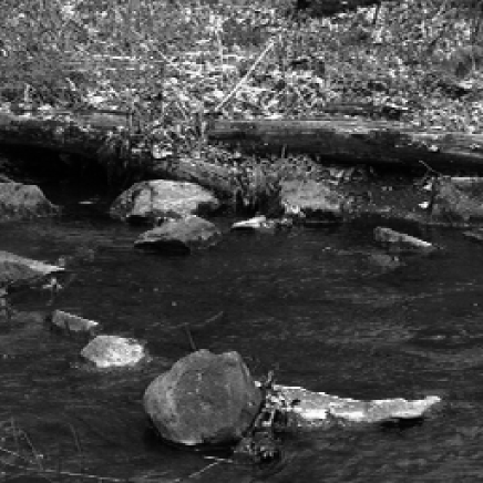
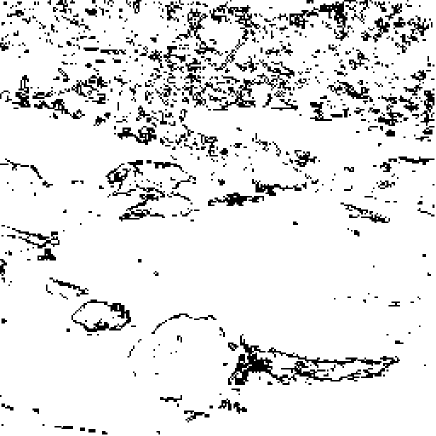
Figure 1: An image from Ruderman’s ensemble (?) and its most singular component (taken as the set of points having a singularity exponent in the interval $h=-0.5\pm 0.05$).

The most singular component is the one with $h=-0.5$, defined within a window of size $\Delta h$. The visualization of this set is very instructive (see Fig. 1). Clearly, the points appear to be associated with the contour of the objects present in the image. This is in agreement with our expectation that the behavior of the measure at these edges should be singular, and as much as possible. But there is something rather surprising: for a sharp, theta-like contrast, with independent values at both sides of the discontinuity, one would have expected an exponent $-1$, which appears as a Dirac $\delta$-function in the density measure $\nabla C$ (see example number 4 in the Appendix). Our interpretation of the minimal value of $h$, $h_{\infty}=-0.5$, is that it reflects the existence of correlations among different fractal components of the images that smoothen the singularities (in particular those of the sharpest edges).

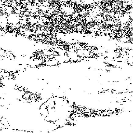
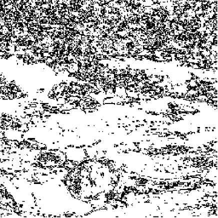
Figure 2: Fractal components with exponents $h=-0.4\pm 0.05$ (above) and $h=-0.3\pm 0.05$ (below) for the same image represented in Fig. 1. Notice the spatial correlations between components with similar singularities.

It is also interesting to observe the fractal components with exponents just above the most singular one. Fig. 2 shows the two next components, defined with $\Delta h=0.05$. A comparison with Fig. 1 shows that pixels in these components are close to pixels in the most singular one. It is also rather clear that the probability that a random ball of size $r$ contains a pixel from the component $F_{h}$ increases with $h$, at least for small values of this exponent. Since this probability scales as shown in eq. (8), this behavior reveals an increase with $h$ of the dimensionality of the fractal components. It is also observed (although not shown in the figures) that the dimensionality starts decreasing beyond $h\approx 0.2$. This is in agreement with the arguments of section 3.3: the singularity spectrum $D(h)$ of the S-L model, which is shown in Fig. 8, reflects this behavior of the fractal components.

The analysis done in this subsection justifies the arguments presented in Section 1. One cannot consider the sharpest edges of an image independently of the other texture structures (i.e. the other fractal components). Luminosity jumps from one roughly constant value to another (statistically independent) constant value are not typical in natural images. The sharpest edges appear correlated with smoother textures, an effect that tends to decrease the strentgh of their singularity exponent, reaching the value $h\sim-0.5$. Standard edge-detection tecniques (?) have not been designed to search for singularities of this strength. Good edge-detection algorithms should be specifically constructed to capture singularities close to $h_{\infty}$.

4.3 Statistical analysis of the measure

We computed the $p$-moments of three different variables related to the measure:

• Bidimensional Edge Content ($\epsilon_{r}$): Following the definition given in eq. (1). This analysis was done using the 25 images of the second dataset. As the variable itself is positive, we computed directly the quantities $\langle\epsilon_{r}^{p}\rangle$.

• Two one-dimensional restrictions of the wavelet projection of the measure ($T^{r}_{\Psi}d\mu$): We considered horizontal ($h$) and vertical ($v$) restrictions of the measure $d\mu$, that is $d\mu^{h}=dx|\frac{\partial\mu}{\partial x}|$ and $d\mu^{v}=dy|\frac{\partial\mu}{\partial y}|$. The appropriate wavelet transforms are denoted by $T^{r}_{\Psi}d\mu^{l}$ ($l=h,v$). As these coefficients need not to be positive (in general $\Psi$ is not positive), we computed the moments of their absolute values, $\langle|T^{r}_{\Psi}d\mu^{l}|^{p}\rangle$.

It is remarkable that the bi-dimensional Edge Content and the two one-dimensional wavelet projections exhibit the scaling properties of SS (eq. 15) and of ESS (eq. 16) (the ESS tests for the three variables are presented in Fig. 3 and 4). This was also observed in (?), although for somewhat different variables: the one-dimensional horizontal and vertical restrictions of the local edge variance. Surprisingly, no matter the particular variable, the exponents $\tau_{p}$ and $\rho(p,2)$ obtained are very similar (see Fig. 5 and those in (?)). Therefore, they should refer to very essential, robust aspects of images.

The S-L model fits very well the experimental exponents (see Fig. 5). It seems then that the multifractal structure underlying the statistical description could be described with the Log-Poisson process, which means that under infinitesimal changes in the scale there are only two possible different types of transformations.

It is really remarkable that for our datasets $\Delta\approx 0.5$ and $D_{\infty}\approx 1$. This means that the most singular component is a collection of lines (the sharp edges present in the image) which can be characterized by their common exponent $-\Delta=-0.5$. But this is precisely the smallest value we observed previously in our wavelet analysis. The statistical approach confirms the result obtained by a local singularity analysis.

The non-linear dependence of $\rho(p,2)$ on $p$ again indicates that the Edge Measure is multifractal. This has to be contrasted with the results by (?, ?) who find that the log-contrast distribution follows a simple classical scaling. It also holds for any derived variable as the gradient (see (?) for details). This particular scaling is related, in that context, with general properties of scale invariance of natural images: the averaging of the contrast does not keep track of the details (e.g., the edges completely contained into the averaging block) and produces a statistically equivalent image. The Edge Content and the wavelet projections, being local averages of a gradient, are able to keep the information about the more complex underlying multifractal structure.

The same authors have also designed an iterative procedure that tends to decompose the image into a gaussian-like piece (local fluctuations of the log-contrast) and an image-like piece (local variances). Such a decomposition would suggest the existence of a multiplicative process for the log-contrast itself where the random variable relating the image at two different levels of the hierarchy is given by the local fluctuations. A closer look to the iterative procedure indicates that this is not the case: independence between the two factors of the process is not guaranteed and also the process is not infinitely divisible.

4.4 Multiaffinity properties of $C$ and $|\nabla C|$

In this section we study the scaling properties for the Linear Increments of the contrast $C(\vec{x})$ and of the measure density $|\nabla C|(\vec{x})$. Our aim is then to check if $C$ and $|\nabla C|$ satisfy the scaling defined in eq. (31). Recalling the connection (the analog of eq. (26) for these two quantities) between local scaling (described by the singularity exponents) and statistical scaling (characterized by the SS exponents), one concludes that the validity of SS implies that multiaffinity holds. We have then done a statistical analysis of the Linear Increments of the contrast and the measure density.

We first computed the $p$-moments of the Linear Increments of both variables, looking for SS and ESS scalings. Let us notice that there is no a priori argument to expect that $\delta_{\vec{r}}C(\vec{x})$ shows SS. On the other hand, since the measure $\mu$ is multifractal (as it was shown in section 4.2) it would be reasonable to expect that $|\nabla C|(\vec{x})$ has a multiaffine behavior. However, this has to be verified explicitly because the multifractality of the measure does not guarantee the multiaffinity of its density, as it was discussed in section 3.4. In fact, our numerical analysis showed that neither $C(\vec{x})$ nor $|\nabla C|(\vec{x})$ have SS. The same is true for ESS, as it is shown in Figs. 6a and  7, where the moments exhibit a rather erratic behavior.

It seems that the failure of SS for $C(\vec{x})$ and $|\nabla C|(\vec{x})$ has to be explained in different terms. In the case of $|\nabla C|(\vec{x})$, this quantity is the measure density and, as it was stated in eq. (10), its convolution with a non-admissible (i.e. positive) wavelet has the same singularities as the measure, eq. (2). This implies that the lack of SS cannot be explained in terms of a polynomial part as described in eq. (37). In fact, a positive wavelet cannot alter the contribution from this polynomial while one observes that the data for $\delta_{\vec{r}}|\nabla C|(\vec{x})$ (Fig. 7) are different from those of $T^{r}_{\Psi}d\mu^{h}$ and $T^{r}_{\Psi}d\mu^{v}$ (Fig. 4).

On the other hand it is plausible that the failure of SS of $\delta_{\vec{r}}C(\vec{x})$ can be attributed to the presence of a polynomial part in $C(\vec{x})$. Differently to what happened with $|\nabla C|(\vec{x})$, when the contrast is convolved with a non-admissible wavelet, SS and ESS are still not present (that is, one observes a similar erratic behavior as in Fig. 6a). The same behavior is observed when $C(\vec{x})$ is convolved with an admissible wavelet with a zero mean. The situation changes drastically when a wavelet with vanishing zero- and first-order moments is used. The result obtained using the second derivative of a gaussian is presented in Fig. 6b, which clearly shows ESS (it also exhibits SS). This can be understood recalling that the possible values of the Hölder exponent of $C(\vec{x})$ are contained in the interval $(0.5,2.4)$ (see eq. (34) and section 4.2). A non-admissible wavelet truncates the detected singularities at the value $h=0$, an admissible one truncates them at $h=1$. The third wavelet considered, with two vanishing moments, truncates the singularities only from $h=2$ and then it covers almost the whole interval (In theory a wavelet with another vanishing moment would be more appropriate, however in practice it is numerically more unstable because the resolution of the wavelet is smaller).

Finally, we also checked that the experimental values of $\tau_{p}$, $\tau_{p}^{\Psi_{{}_{C}}}$ and $\tau_{p}^{\Psi_{{}_{\nabla C}}}$ satisfy the relation given in eq. (43).

5 Discussion

We have shown that in natural scenes pixels are arranged in non-overlapping classes, the fractal components of the image, characterized by the behavior of the contrast gradient under changes in the scale. In each of these classes this quantity exhibits a distinct power law behavior under scale transformations, what indicates that there is no a well-defined scale for the isolated components but that at the same time the scene is not scale invariant globally.

This result implies that a given image is composed of many different spatial structures of the contrast associated to the fractal components, which can be arranged in a hierarchical way. In fact, how sharp or soft a change in contrast is at a given point can be quantified in terms of the value of the scaling exponent at that site. The smaller the exponent the sharper the local change in contrast is.

More precisely, we have dealt with two basic quantities: the contrast $C(\vec{x})$ and the edge measure $\mu$, which density is the modulus of the contrast gradient $|\nabla C|(\vec{x})$ (see eq. (2)). Closely related to the measure, we can define the edge content of a region $A$ of the image (eq. (3)), which quantifies how much the contrast gradient deviates from being uniformly distributed inside the region $A$. This is a suitable definition to study the local behavior of the contrast gradient. As the size of $A$ is reduced, some contributions of the contrast gradient to the edge content are left outside this region. Under an infinitesimal change in the scale very often these contributions are small, but sometimes it does happen that a small change in the scale produces a large change in the edge content. This is due to singularities in the contrast gradient. As a consequence of this, the edge content (and the measure) exhibits large spatial fluctuations. The edge content can have different singularities at neighbouring points, characterized by a power-law behavior with exponents $h(\vec{x})$ which depend on the site, eq. (6). This means that the measure is multifractal, as it has been explicitly verified in this work.

The set of pixels with the same value of $h(\vec{x})$ defines a particular spatial structure of contrast: the fractal component $F_{h}$. The smallest $h(\vec{x})$ is the sharpest the contrast gradient at the pixel $\vec{x}$ is. Its minimal value was, for our dataset, $h_{\infty}=-0.5$. Another question refers to the fractal dimension $D_{\infty}$ of this component. One finds $D_{\infty}=1$ (?), and when this component is extracted from the image one checks that it corresponds to the boundaries of the objects in the scene. The associated contrast structure is made of the sharpest edges of the image. The other, less singular components represent softer contrast structures inside the objects. It is also observed that there are strong spatial correlations between fractal components with similar exponents.

We have also shown how to extract the fractal components from the image. To do this one needs a suitable technique to compute the scale behavior at a given pixel. A wavelet projection (?, ?) seems to be the correct way to perform this analysis, since it provides a way of interpolating scale values which are not an integer number of pixels. Our approach differs from the one followed in those references in several aspects, but in particular in that we have been here interested in the characterization of the whole set of fractal components.

We remark the important fact that the multifractal can be explained by a model with only two parameters (e.g. $\beta$ and $\Delta$). This had been noticed before in terms of a variable that integrates the square of the derivative of the contrast along a segment of size $r$, both taken either in the horizontal or in the vertical direction (?) . This quantity admits the interpretation of a local linear edge variance. We have seen that the same model is valid for many other quantities, some of them more general and natural.

The basic idea of the model is that the contrast gradient has singularities that under an infinitesimal change in the size of $A$ produce a substantial change in the edge content inside that region. The simplest stochastic process to assign a value to this change is a binomial distribution, eq (20): its more likely value is very small, but with small probability this change is given by the parameter $\beta$, which for our dataset is about $0.5$. The other parameter of the model, $\Delta$, measures the strength of the singularity. The geometrical locus of these singularities is the most singular fractal component. For a finite scale transformation this process becomes Log-Poisson. The model appeared before in other problems (?).

In a sense, the most singular component conveys a lot of information about the whole image. The two model parameters can be obtained by analyzing properties of this particular class of pixels: its dimension ($D_{\infty}$) and the scale exponent of the edge content ($\Delta=-h_{\infty}$). In turn, these two parameters completely define the whole dimension spectrum in the Log-Poisson model. It is then very plausible that other components have a great deal of redundancy with respect to the most singular one.

This hierarchical representation of spatial structure can be used to predict specific feature detectors in the visual pathways. We conjecture that the most singular component contains highly informative pixels of the images that are responsible for the epigenetic development leading to the adaptation of receptive fields. Learning of the statistical regularities (?) present in this portion of visual scenes (using for instance the algorithm in (?)), would give relevant predictions about the structure of receptive fields of cells in the early visual system.

Appendix A Characterization of the singularities of simple functions

It is instructive to compute the singularity exponents defined in eq. (30) for several simple functions.

1. Continuous functions: If a function $f(\vec{x})$ is continuous at a given point $\vec{x}$, the value of $f$ at $\vec{y}$ should be rather close to $f(\vec{x})$ provided $\vec{y}$ is close to $\vec{x}$; then $|f(\vec{y})|<|f(\vec{x})|+\epsilon$ so $|f(\vec{x})-f(\vec{y})|<2|f(\vec{x})|+\epsilon=A$. That is, $f$ is Hölder of exponent $0$ at $\vec{x}$.

2. Smooth functions with continuous, non-vanishing first derivative: Using the Taylor expansion, $f(\vec{x})-f(\vec{y})=\nabla f(\vec{y}_{0})\cdot(\vec{x}-\vec{y})$ with $\vec{y}_{0}$ a point between $\vec{x}$ and $\vec{y}$. Let us call $A=\max|\nabla f(\vec{y}_{0})|>0$, so $|f(\vec{x})-f(\vec{y})|<A|\vec{x}-\vec{y}|$. That is, $f$ is Hölder of exponent $1$ at $\vec{x}$.

   Analogously, any function $f$ having $n-1$ vanishing derivatives at a point $\vec{x}$ and a non-vanishing continuous $n$-th derivative, is Hölder of exponent $n$ at $\vec{x}$.

3. $\theta$-function: The $\theta(x)$ function is given by

   $$\theta(x)\;=\;\left\{\begin{array}[]{cc}0&x<0\\ 1&x>0\\ \mbox{undefined}&x=0\end{array}\right.$$

   Since for $x\neq 0$ the increments are zero (for small enough displacement) it is Hölder of any order. For $x=0$ we make use of the property that $f$ is Hölder of exponent $h$ at a given point if and only if its primitive $F$ is Hölder of exponent $h+1$ at the same point.

   One possible primitive $F(x)$ of $\theta(x)$ is the following:

   $$F(x)\;=\;\left\{\begin{array}[]{cc}0&x<0\\ x&x\geq 0\\ \end{array}\right.$$

   which is a continuous function. The increments $|F(0)-F(r)|=|F(r)|=F(r)$ are thus immediate, and obviously $F(r)<|r|$. Moreover, it is also clear that the maximal $h$ such that $|F(0)-F(r)|<A|r|^{h}$ is $h=1$. Thus, $F$ has Hölder exponent 1 at $x=0$ and therefore $\theta(x)$ has Hölder exponent 0 at $x=0$.

4. $\delta$-function: The Dirac’s $\delta$-function is in fact a distribution. Anyway, it is possible to define the Hölder exponent of distributions attending to the fact that any distribution can be expressed as a finite order derivative of a bounded function. So, if the $n$-th order primitive of a distribution is a Hölder function of exponent $h$ at a given point, the distribution is Hölder of exponent $h-n$ at the same point.

   Since the $\delta(x)$ distribution vanishes in $x\neq 0$ the only non-trivial point is $x=0$. Since the $\delta$ is the derivative of $\theta(x)$ and this has Hölder exponent $0$ at $x=0$, one concludes that the $\delta(x)$ has Hölder exponent $-1$ at $x=0$

Figure 3: Test of ESS for the bidimensional edge content $\epsilon_{r}$. The graphs represent the logarithm of its moments of order 3, 5 and 7 versus the logarithm of the second order moment, for distances $r=4$ to $r=64$ pixels, that is, about an order of magnitude smaller than the image size. This upper bound is needed both to consider values of $r$ small enough compared to the size of the images and to be able to use moments of high order as $p=7$. The data corresponds to the second image ensemble. According to eq. (16) these graphs should be straight lines; the best linear fits are also represented. Except for lower cut-off effects at very small distances, the scaling law is well verified.

Figure 4: Test of ESS for a) $T^{r}_{\Psi}d\mu^{h}$ and b) $T^{r}_{\Psi}d\mu^{v}$. The graphs represent the logarithm of the moments of order 3, 5 and 7 for both variables versus the logarithm of the corresponding second order moment. The scales range from $r=4$ to $r=64$ pixels. The first dataset was used in this computation. The corresponding best linear fits are also represented. Except for lower and upper cut-off effects at small and large distances, the scaling law verifies well. Although the test is not shown here, SS also holds for these variables.

$\rho(p,2)$    $a$                                $b$                                $c$

   $p$                                $p$                                $p$

Figure 5: ESS exponents $\rho(p,2)$ for a) the bidimensional edge content $\epsilon_{r}$ , b) the horizontal wavelet transform $T^{r}_{\Psi}d\mu^{h}$ and c) the vertical one, $T^{r}_{\Psi}d\mu^{h}$. The convolution function $\Psi$ was taken to be a gaussian function. Each value of $\rho(p,2)$ was obtained by linear regression of the logarithm of the $p$-th moment versus the logarithm of the second moment, for $r$ between 8 and 32. The solid line represents the fit with the Log-Poisson process. The best fit is obtained with a) $\beta=0.52\pm 0.05$ b) $\beta=0.55\pm 0.06$ and c) $\beta=0.5\pm 0.07$ The SS parameters $\tau_{2}$ were also calculated; they turned out to be a) $\tau_{2}=-0.26\pm 0.06$ , b) $\tau_{2}=-0.25\pm 0.06$ and c) $\tau_{2}=-0.25\pm 0.08$.

Figure 6: Test of ESS for a) the horizontal linear increment of the contrast, $\delta_{r\vec{i}}C$ and b) the horizontal wavelet coefficient $|T^{r}_{\Psi}C^{h}|$ ($\Psi$ was taken as the second derivative of a gaussian); the first dataset was used and the range of scales was from $r=4$ to $r=64$. ESS is not present for $\delta_{r\vec{i}}C$, but it is clearly observed for the wavelet transform (notice the presence of the cut-offs due to numerical effects). Note that the scale of the axes in a) and b) is different.

Figure 7: Test of ESS for a) horizontal linear increment of $|\nabla C|$, $\delta_{r\vec{i}}|\nabla C|$ and b) vertical linear increment of the same function, $\delta_{r\vec{j}}|\nabla C|$. The first dataset was used and the scales were taken ranging from $r=4$ to $r=64$ pixels. Again, these variables do not have ESS. The corresponding wavelet projections are shown in Fig. 4 where one can see that ESS holds.

Figure 8: Singularity spectrum of the Log-Poisson model for $\beta=0.5$ and $\tau_{2}=-0.25$. For these values $D_{\infty}=1.$ and $\Delta=0.5$ (see text)