Unconventional antiferromagnetic correlations of the
doped Haldane gap system Y₂BaNi_1-xZn_xO₅

Abstract

We make a new proposal to describe the very low temperature susceptibility of the doped Haldane gap compound Y₂BaNi_1-xZn_xO₅. We propose a new mean field model relevant for this compound. The ground state of this mean field model is unconventional because antiferromagnetism coexists with random dimers. We present new susceptibility experiments at very low temperature. We obtain a Curie-Weiss susceptibility $\chi(T)\sim C/(\Theta+T)$ as expected for antiferromagnetic correlations but we do not obtain a direct signature of antiferromagnetic long range order. We explain how to obtain the “impurity” susceptibility $\chi_{\rm imp}(T)$ by subtracting the Haldane gap contribution to the total susceptibility. In the temperature range [1 K, 300 K] the experimental data are well fitted by $T\chi_{\rm imp}(T)=C_{\rm imp}\left(1+T_{\rm imp}/T\right)^{-\gamma}$. In the temperature range [100 mK, 1 K] the experimental data are well fitted by $T\chi_{\rm imp}(T)=A\ln{(T/T_{c})}$, where $T_{c}$ increases with $x$. This fit suggests the existence of a finite Néel temperature which is however too small to be probed directly in our experiments. We also obtain a maximum in the temperature dependence of the ac-susceptibility $\chi^{\prime}(T)$ which suggests the existence of antiferromagnetic correlations at very low temperature.

I Introduction

Disordered low dimensional spin systems are currently the focus of both experimental and theoretical interest. A very powerful theoretical technique used to describe these systems consists in iterating a real space renormalization group (RG) in which high energy degrees of freedom are progressively frozen out. The cluster RG was initially proposed by Dasgupta an Ma in the early 80’s [1] and applied soon after by Bhatt and Lee to a three dimensional (3D) model intended to describe Si:P [2]. In a series of articles, Fisher applied the cluster RG to disordered 1D antiferromagnets, including the random Ising chain in a transverse magnetic field and the random antiferromagnetic spin-$1/2$ chain [3]. In these models, the cluster RG is so powerful that it allows to obtain exact results regarding two aspects of the problem: (i) the correlation functions associated with the approach of a random singlet fixed point; and (ii) the approach of a quantum critical point. It is fair to say that there exists now a detailed theoretical understanding of all random spin models in one dimension [4, 5, 6, 7], and even in higher dimensions [8]. Some models do not have a quantum critical point [3, 7] while other models have a zero temperature phase transition which is controlled by the strength of disorder [3, 4, 5, 6]. In particular, weak disorder is irrelevant in the random spin-$1$ chain but there is a quantum critical point at a critical disorder $d_{c}$. For $d>d_{c}$, the random spin-$1$ chain behaves like a random singlet [5, 6], namely, the strength of disorder increases indefinitely as the temperature is scaled down, which is known as an “infinite randomness” behavior [8].

On the experimental side, it has become possible to fabricate low dimensional oxides in the last five years, and dope them in a well controlled fashion. As a consequence, these systems give the unique opportunity of exploring the introduction of disorder in a spin gap state. It would be erroneous however to think that there exists a straightforward relation between these experiments on quasi one dimensional oxides and the 1D models that have been widely studied by theoreticians in which the disorder is introduced in the form of random bonds. In fact, the 1D models with random bonds are not directly applicable to experiments. The reason is that the relevant models should incorporate the following realistic constraints:

• Doping in quasi one dimensional oxides is introduced by substitutions, and not in the form of random exchanges. The usual random bond models are not the most relevant ones.

• The temperature is finite in the experiments, even though often very small.

• The realistic systems are not 1D. Interchain couplings become relevant at low temperature and can change the physics drastically.

The problem is then to determine to what extent realistic models incorporating these three constraints still behave like the original 1D random bond models.

One of the recently discovered low dimensional oxides is CuGeO₃ [9] which has a spin-Peierls transition at $T_{SP}\simeq 14$ K below which the CuO₂ chains dimerize with the appearance of a gap in the spin excitation spectrum. Soon after the discovery experimentalists began to study the effects of various substitutions on this inorganic compound. For instance, it is possible to substitute a small fraction of the Cu sites (being a spin-$1/2$ ion) by Ni (being a spin-$1$ ion) [10] or Co (being a spin-$3/2$ ion) [11]. It is possible to substitute Cu by the non magnetic ions Zn [12, 13, 14] or Mg [15]. It is also possible to substitute some Ge sites (being outside the CuO₂ chains) with Si [16]. The general feature emerging from the detailed experimental studies of the various substitutions is the existence of antiferromagnetism at low temperature. It has even been shown experimentally by Manabe et al. that at low doping concentrations, the Néel temperature behaves like $\ln{T_{N}}\sim 1/x$ [17], therefore suggesting that there is no critical concentration associated with the onset of antiferromagnetism.

The Haldane gap is another example of a spin gap in a low dimensional antiferromagnet [18]. Two inorganic Haldane gap antiferromagnets have been discovered recently: PbNi₂V₂O₈ which has a spin gap $\Delta\simeq 28$ K [19], and Y₂BaNiO₅ which has a spin gap $\Delta\simeq 100$ K [20]. The substitution of the spin-$1$ Ni sites of PbNi₂V₂O₈ with Mg (a non magnetic ion) generates long range antiferromagnetism at low temperature. The situation with Y₂BaNiO₅ is not so well established. Previous works have failed to find long range antiferromagnetic order at low temperature [21, 22, 23, 24]. In particular $\mu$SR experiments at $50$ mK in Ref. [23] have reported a paramagnetic relaxation with a Mg doping of $1.7\%$ and $4.1\%$. We report here a study of the effect of Zn substitutions in Y₂BaNiO₅. In agreement with Ref. [23], we do not find antiferromagnetic long range order down to $100$ mK. But from the analysis of the experimental ac- and dc-susceptibility we deduce the existence of 3D antiferromagnetic correlations which rule out the “1D quantum criticality” scenario represented on Fig. 1-(a).

FIG. 1.: Two possible scenarii for Y₂BaNi_1-xZn_xO₅. In (a) there are no interchain couplings ($J_{\perp}=0$) and the physics is governed by the approach to the quantum critical point of the disordered Haldane gap chain. A power-law susceptibility is expected in this situation at low temperature (Griffiths behavior). In (b) interchain couplings play a relevant role and generate an unconventional phase in which antiferromagnetism coexists with random dimers. The approach to the Néel transition is controlled by the establishment of antiferromagnetic correlations. The purpose of the article is to show that the situation (b) can apply to Y₂BaNi_1-xZn_xO₅.

There have been several attempts to find a theoretical description of doped spin-Peierls systems. Fukuyama, Tanimoto and Saito have made the first proposal [25]. Another route has been followed by Fabrizio, Mélin and Souletie. In a series of article [26, 27, 28], these authors have provided a detailed scenario for disordered antiferromagnetism. Appealing aspects of their approach is that the doped spin-Peierls and the doped Haldane gap systems can be described in the same framework [28], and the model appears to be fully compatible with experiments. The relevant physics is determined by comparing two energy scales:

• The coherence temperature $T^{*}=\Delta\exp{[-1/(x\xi)]}$ which controls the formation of singlet correlations.

• The Stoner temperature $T_{\rm Stoner}=J_{\perp}x\xi$ which controls the formation of 3D antiferromagnetic correlations.

In these expressions, $x$ is the doping concentration, $\Delta$ is the spin gap, $\xi$ is the correlation length of the pure gaped system, and $J_{\perp}$ is the interchain coupling. The specificity of Y₂BaNi_1-xZn_xO₅ is that $T^{*}>T_{\rm Stoner}$ while $T^{*}\ll T_{\rm Stoner}$ in Cu_1-xZn_xGeO₃ and Pb(Ni_1-xMg_x)V₂O₈ (see Refs. [26, 28]). As a consequence in Y₂BaNi_1-xZn_xO₅, 3D antiferromagnetic correlations coexist with non magnetic random dimer correlations (see Fig. 1–(b)). Based on the calculation of the exchange coupling two spin-$1/2$ moments associated to the same impurity presented in Ref. [29], we propose a mean field model relevant for Y₂BaNi_1-xZn_xO₅. From this mean field model we can obtain new insights in the nature of the low temperature phase, and compare the model to very low temperature susceptibility experiments.

The article is organized as follows. The model is presented in section II. Section III is devoted to calculate the susceptibility and discuss the nature of the low temperature phase. In section IV we present and analyze the very low temperature susceptibility experiments. Concluding remarks are given in section V.

II The model

A Defects in spin-Peierls and Haldane gap systems

FIG. 2.: Schematic representation of two non magnetic impurities inserted in a spin-$1$ chain. The thick arrows are the spin-$1$ moments. The thin arrows are the “edge” spin-$1/2$ moments. The exchange coupling the two spins ${\bf S}_{1}$ and ${\bf S}_{2}$ is given by (1) and (2). We have represented an even segment. The exchange between ${\bf S_{1}}$ and ${\bf S}_{2}$ is therefore antiferromagnetic.

FIG. 3.: Schematic representation of two non magnetic impurities inserted in a spin-Peierls chain. (a) corresponds an even segment with two spin-$1/2$ moments. In this case the exchange (1), (2) between ${\bf S}_{1}$ and ${\bf S}_{2}$ is the same as for the Haldane gap chain. (b) corresponds to an odd segment with one spin-$1/2$ moment. (c) corresponds to an even segment with no spin-$1/2$ moment.

The model that should be used to describe doped Haldane gap compounds is well established. The introduction of a non-magnetic impurity in a spin-$1$ chain generates a pair of “edge” spin-$1/2$ moments on either side of the impurity [30, 31, 32, 33] (see Fig. 2). The spin-$1/2$ moments associated with two neighboring impurities interact with the Hamiltonian

$${\cal H}=J(l){\bf S}_{1}.{\bf S}_{2},$$ (1)

where the exchange is ferromagnetic for odd segments (${\bf S}_{1}$ and ${\bf S}_{2}$ are in the same sublattice), and antiferromagnetic for even segments (${\bf S}_{1}$ and ${\bf S}_{2}$ are in a different sublattice):

$$J(l)=(-)^{l}\Delta\exp{\left(-\frac{l}{\xi}\right)},$$ (2)

where $\xi$ is the correlation length associated to the Haldane gap. We note $J_{2}$ the ferromagnetic exchange coupling between two spins associated with the same impurity. Quantum chemistry calculations indicate that $J_{2}$ is smaller than the interchain coupling $J_{\perp}$ in Y₂BaNi_1-xZn_xO₅ [29]. The authors of Ref. [29] have obtained $J_{\perp}\simeq 0.2-0.9$ K and $J_{2}<0.1$ K. This means that there is no temperature range in which the effective low energy model can be considered as one dimensional. On the contrary, when $T$ is above $J_{2}\sim J_{\perp}$ the system can be represented by a model having $J_{2}=J_{\perp}=0$. When $T$ is below $J_{2}\sim J_{\perp}$ the system develops directly three-dimensional correlations. As a consequence we will use a model with $J_{2}=0$ but with finite interchain correlations that will be treated in mean field. We note that the role of interchain correlations was already pointed out in Ref. [24]. On the basis of DMRG calculations for open segments, the authors of Ref. [24] could obtain a good agreement between the model and the experiments on Y₂BaNi_1-xZn_xO₅ above 4 K. The deviations occurring in the temperature range [2 K, 4 K] have been attributed to interchain correlations which play a central role in the model developed here.

It will be fruitful to make a qualitative comparison with doped spin-Peierls systems, which are closely related to the doped Haldane gap systems [26]. Non magnetic impurities introduced in a spin-Peierls system generate unpaired spin-$1/2$ moments (see Fig. 3). Depending on the parity of the length of the segment and on the dimerization pattern, there can be zero, one or two spin-$1/2$ moments. If there are two spin-$1/2$ moments (see Fig. 3-(a)) the exchange (1) and (2) is the same as for the Haldane gap chain. To discuss the qualitative physics, we will make the approximation of including only the segments on Fig. 3-(a) that give rise to two spin-$1/2$ moments and neglect the other segments.

B Role of interchain interactions

Interchain interactions can be described by introducing a correlation length $\xi_{\perp}$ in the transverse direction. In two dimensions, the effective low energy Hamiltonian is a sum over all pairs of spins [26]:

$${\cal H}=\sum_{\langle i,j\rangle}J_{i,j}{\bf S}_{i}.{\bf S}_{j},$$ (3)

where the exchange between the spin ${\bf S}_{i}$ at coordinates $(x_{i},y_{i})$ and the spin ${\bf S}_{j}$ at coordinates $(x_{j},y_{j})$ is given by

$$J_{i,j}=(-)^{r_{x}+r_{y}}\Delta\exp{\left(-\sqrt{\left(\frac{r_{x}}{\xi}\right)^{2}+\left(\frac{r_{y}}{\xi_{\perp}}\right)^{2}}\right)},$$ (4)

where $r_{x}=x_{i}-x_{j}$ and $r_{y}=y_{i}-y_{j}$. It has been shown from the RG approach in 2D that the Hamiltonian defined by (3) and (4) in two dimensions has a finite randomness behavior [26]. This indicates the existence of long range antiferromagnetism. In the present work, we do not address directly the model defined by (3) and (4) in 2D. Instead we propose that Y₂BaNi_1-xZn_xO₅ can be described by a mean field model in which we introduce a coupling to a molecular field $-h_{s}\sum_{i}S_{i}^{z}$. The value of the molecular field is equal to the strength of antiferromagnetic correlations, which can be obtained from the susceptibility experiments in section IV. Since we use a mean field model, we cannot make the distinction between “antiferromagnetic long range order” and “antiferromagnetic correlations with a finite (but possibly large) correlation length”. For the sake of simplicity we assume that the staggered molecular field is uniform. But our approach can be extended to incorporate a distribution of molecular fields. The distribution of molecular fields can be calculated in a self-consistent way by imposing that the exchange field distribution is identical to the staggered moment distribution, up to a proportionality factor related to the strength of interchain correlations.

C Summary of the article

FIG. 4.: Schematic representation of the ground state obtained from the mean field approach. The even segments are coupled into non magnetic random dimers. The other spins give rise to antiferromagnetic long range order.

Our strategy will be to solve the cluster RG in the presence of a molecular field for a model having $J_{2}=0$ (see Fig. 2). Because this model reduces to a sum of independent two-spin Hamiltonians, we call this model a “two-spin model”. The Hamiltonian is given in Appendix A (see Eqs. A1, A5).

The mean field model shows that antiferromagnetism coexists with random dimers at low temperature (see section III) which are due to the even segments coupled antiferromagnetically. This coexistence can be understood on a simple basis: at low temperature the even segments are coupled into non magnetic dimers while the odd segments are coupled into spin-$1$ objects. Interchain interactions generate antiferromagnetic correlations among the spin-$1$ moments. The spin-$1$ moments can eventually order antiferromagnetically (see Fig. 4).

III Nature of the low temperature phase: coexistence between antiferromagnetism and random dimers

A Susceptibility of the two-spin model

FIG. 5.: Temperature dependence of the susceptibility of the two-spin model, with the parameters relevant for Y₂BaNiO₅: $\xi=6$, $\Delta=100$ K, $h_{s}=0.3$ K, $x=8\%$. We have also shown separately the contribution of even segments (coupled antiferromagnetically) and odd segments (coupled ferromagnetically).

FIG. 6.: Temperature dependence of $T\chi(T)$ for the two-spin model coupled to a molecular field. The parameters are identical to Fig. 5. For each doping concentration we have shown by a dashed line the temperature dependence of the RG susceptibility (11) which does not contain a coupling to the molecular field.

The exact treatment of the two-spin model is briefly given in Appendix A. The total susceptibility is obtained by averaging Eq. A4 over all possible realizations of disorder, i.e. over all possible bond lengths:

$$\langle\langle\chi(T)\rangle\rangle=\sum_{l=1}^{+\infty}{\cal P}(l)\chi(l,T).$$

The bond length distribution is ${\cal P}(l)=x(1-x)^{l-1}\simeq x\exp{(-xl)}$, with $x$ the impurity concentration. The temperature dependence of the susceptibility is shown on Fig. 5. A maximum occurs in the susceptibility when the temperature is of the order of interchain interactions, below which the susceptibility decreases to zero. As it can be seen in Fig. 5, the contribution of even segments (being coupled antiferromagnetically) is much smaller than the contribution of odd segments (being coupled ferromagnetically). The reason is that even segments tend to form dimers which do not couple to a uniform magnetic field. Both types of segments couple to the staggered molecular field, which is why the susceptibility on Fig. 5 has a maximum when $T\simeq h_{s}$ and decreases to zero at lower temperature.

The temperature dependence of $T\chi(T)$ is shown on Fig. 6 for three doping concentrations corresponding to the experiments in section IV. At high temperature we recover the Curie constant of free spin-$1/2$ moments with a concentration $2x$:

$$\left[T\chi(T)\right]_{T=\Delta}=2x\frac{S(S+1)}{3}={x\over 2}.$$

At low temperature, $T\chi(T)$ is exponentially small because of the coupling to the staggered molecular field.

B Renormalization of the two-spin model

FIG. 7.: Temperature dependence of the two order parameters $\varphi_{\rm AF}(T)$ and $\varphi_{\rm dim}(T)$ with the parameters relevant for Y₂BaNiO₅ (see Fig. 5). The energy scale corresponding to random dimer formation is larger than the energy scale at which antiferromagnetism appears. The calculation corresponds to the RG procedure presented in section III B. The parameters are given on Fig. 5.

FIG. 8.: Temperature dependence of the two order parameters $\varphi_{\rm AF}(T)$ and $\varphi_{\rm dim}(T)$ with the parameters relevant for CuGeO₃ (see Fig. 10). Dimer formation plays little role here. The calculation corresponds to the RG procedure presented in section III B. The parameters are $\Delta=44.7$ K, $\xi=10$, $h_{s}=0.03$ and $x=0.001$. The values of $h_{s}$ and $x$ are deduced from the low doping experiments in Ref. [17].

FIG. 9.: Antiferromagnetic and dimer order parameters with the parameters relevant for Y₂BaNiO₅ (see Fig. 5). The calculation corresponds to a direct diagonalization of the two-spin Hamiltonian, subject to a temperature-independent staggered molecular field.

FIG. 10.: Antiferromagnetic and dimer order parameters with the parameters relevant for CuGeO₃. The parameters are shown on Fig. 8.

Now we implement RG transformations for the two-spin model coupled to a molecular field $h_{s}$ and having $J_{2}=0$. At low temperature ($T<h_{s}$) the spins are either frozen into dimers, or align antiferromagnetically. The coexistence between the two orders is therefore very natural in this framework. The detailed calculation in presented in Appendix B.

1 Order parameters

The temperature dependence of the two order parameters is shown in Fig 7 for Y₂BaNiO₅ and in Fig. 8 for CuGeO₃. It is clear that dimer formation is not important in CuGeO₃ while it plays a crucial role in Y₂BaNiO₅. To check that this coexistence is not an artifact of the cluster RG, we have made a similar analysis with the direct diagonalization of the two-spin model (see Appendix A). Considering and eigenstate of the form $x|+,-\rangle+y|-,+\rangle$, we define

$$\varphi_{\rm AF} = x^{2}-y^{2}$$ (5)

$$\varphi_{\rm dim} = {1\over 2}(x-y)^{2}\$$ (6)

as the order parameters associated to antiferromagnetism and dimer formation. In the presence of a pure dimer ordering, one has $x=-y=1/\sqrt{2}$, leading to $\varphi_{\rm AF}=0$ and $\varphi_{\rm dim}=1$. In the presence of a pure antiferromagnetic ordering, one has $x=1$ and $y=0$, leading to $\varphi_{\rm AF}=1$ and $\varphi_{\rm dim}=1/2$. The qualitative behavior is similar to the RG treatment (see Figs. 9 and 10), therefore supporting our proposal that random dimers coexist with antiferromagnetism in the mean field model relevant for Y₂BaNiO₅.

2 RG Susceptibility

The RG susceptibility in the temperature range $2h_{s}<T<\Delta$ is obtained as the sum of the contribution of the spin-$1/2$ and spin-$1$ moments that have not been decimated. We note $n_{S}(T)$ the density of spin-$S$ moments (number of spin-$S$ moments per unit length). The total susceptibility reads

$$\chi(T)=\sum_{S}n_{S}(T)\frac{S(S+1)}{3T}.$$ (7)

As far as even segments are concerned, we find (see Appendix B) $n_{1/2}^{({\rm even})}(T)=x\left(T/\Delta\right)^{x\xi}$, from what we obtain the susceptibility of even segments:

$$\chi_{\rm even}(T)=\frac{x}{4T}\left(\frac{T}{\Delta}\right)^{x\xi}.$$ (8)

As far as odd segments are concerned, we obtain from Appendix B: $n_{1/2}^{({\rm odd})}(T)=x\left(T/\Delta\right)^{x\xi}$, and $n_{1}^{({\rm odd})}(T)={x\over 2}\left[1-\left(T/\Delta\right)^{x\xi}\right]$, from what we deduce

$$\chi_{\rm odd,1/2}(T) = \frac{x}{4T}\left(\frac{T}{\Delta}\right)^{x\xi}$$ (9)

$$\chi_{\rm odd,1}(T) = \frac{x}{3T}\left[1-\left(\frac{T}{\Delta}\right)^{x\xi}\right].$$ (10)

The total susceptibility is $\chi_{\rm tot}(T)=\chi_{\rm even}(T)+\chi_{\rm odd,1/2}(T)+\chi_{\rm odd,1}(T)$:

$$\chi_{\rm tot}(T)={x\over 3T}\left[1+{1\over 2}\left({T\over\Delta}\right)^{x\xi}\right],$$ (11)

where the temperature $T$ is such that $2h_{s}<T<\Delta$.

We have presented on Fig. 6 a comparison between the direct diagonalizations and the RG susceptibility of the two-spin model. We see from this figure that the value of $T\chi(T)$ obtained from the cluster-RG is very close to the exact diagonalizations in the temperature range $2h_{s}<T<\Delta$. We can make the following remarks:

• In the absence of the staggered molecular field (i.e. in the absence of interchain couplings) $T\chi(T)$ tends to a constant when $T\rightarrow 0$. This constant is equal to the Curie constant of spin-$1$ moments with a concentration $x/2$:

  $$\left[T\chi(T)\right]_{T=0}={x\over 2}{S(S+1)\over 3}={x\over 3}.$$ (12)

• In the presence of a uniform staggered molecular field, the susceptibility is exponentially small at low temperature:

  $$T\chi_{\parallel}(T)\sim\exp{\left(-{h_{s}\over T}\right)}.$$ (13)

  if the applied magnetic field is parallel to the molecular field. If the applied magnetic field is perpendicular to the molecular field, the susceptibility tends to a constant:

  $$T\chi(T)\sim\chi_{0}T.$$ (14)

  If the sample is a powder as in the experiments presented in section IV, the susceptibility given by Eqs.(13), (14) should be averaged over all directions and we obtain

  $$T\chi_{\rm av}(T)\sim\lambda\chi_{0}T,$$ (15)

  where $\lambda$ is smaller than unity.

Therefore a relevant question for experiments is to determine whether $T\chi(T)$ tends to a constant (like in Eq. (12)) or tends to zero (like in Eq. (15)) in the limit of zero temperature. From the answer to this question we can determine whether 3D antiferromagnetic correlations are important in Y₂BaNi_1-xZn_xO₅.

IV Experiments

$x$	$\Theta$	$C$	$T_{\rm imp}$	$C_{\rm imp}$	$\Delta_{1}$	$C_{1}$	$\Delta_{2}$	$C_{2}$	$T_{c}$	$A$
	(K)	($10^{-3}$ eum.K	(K)	(eum.K	(K)	(eum.K	(K)	(eum.K	(K)	($10^{-3}$eum
		/Ba.mol)		/Ba.mol)		/Ba.mol)		/Ba.mol)		/Ba.mol)
0.00	0.222	6.44	71.6	0.017	534	1.07	138	0.267	0.021	3.20
0.04	0.498	26.0	3.25	0.032	451	0.995	116	0.19	0.046	13.2
0.06	0.677	34.4	3.13	0.040	494	1.01	122	0.207	0.052	15.9
0.08	0.922	41.6	3.71	0.046	486	0.965	120	0.19	0.054	17.2

TABLE I.: Parameters of the best fits of the susceptibility data. $\Theta$ and $C$ are the parameters of the Curie-Weiss fit (16) in the temperature range [1 K, 10 K]. $T_{\rm imp}$ and $C_{\rm imp}$ are the parameters of the power-law fit (20) of the “impurity” contribution to the susceptibility in the temperature range [1 K, 300 K]. $\Delta_{1}$, $C_{1}$, $\Delta_{2}$ and $C_{2}$ are the parameters of the two-exponential fit of the Haldane gap susceptibility (see Eq. (18)). $T_{c}$ and $A$ are the parameters of the fit given by Eq. (21) in the temperature range [100 mK, 1 K].

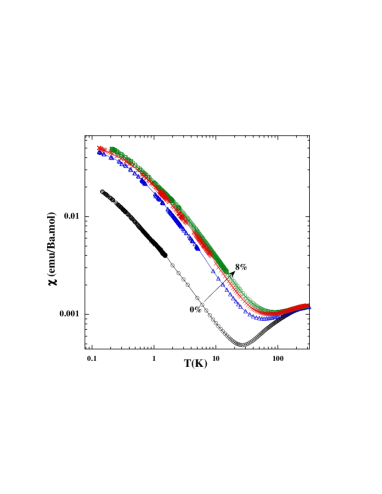
FIG. 11.: Temperature dependence of the dc-susceptibility of the four samples ($x=0.00$, $x=0.04$, $x=0.06$, $x=0.08$) with a magnetic field $H=0.1$ T. This is a log-log plot.

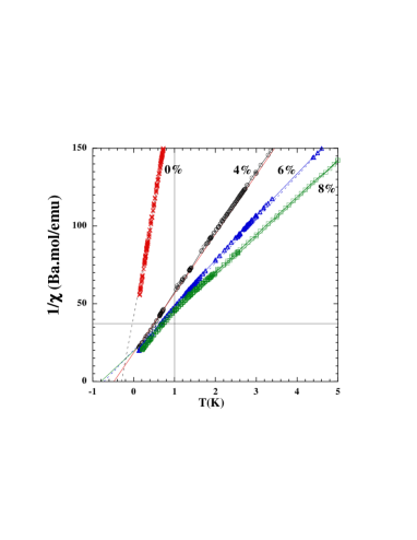
FIG. 12.: $1/\chi$ versus $T$ for $x=0.00$, $x=0.04$, $x=0.06$ and $x=0.08$. The dashed line are linear fits valid in the temperature range [1 K, 10 K]. The fits intercept the $T$ axis at a negative temperature which is a signature of antiferromagnetic correlations.

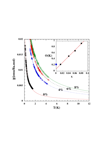
FIG. 13.: Magnetic susceptibility versus temperature at low temperature for $x=0.00$, $x=0.04$, $x=0.06$ and $x=0.08$. The curves have been fitted to the Curie-Weiss law (16) over the temperature range [1 K, 10 K]. The insert shows how $\Theta$ depends on the doping concentration $x$. To incorporate the existence of a finite level of disorder in the undoped sample, we made the replacement $x=0.00\rightarrow x=0.014$.

We investigated the very low temperature susceptibility of the doped Haldane gap compound Y₂BaNi_1-xZn_xO₅. We have performed ac- and dc-susceptibility measurements with a SQUID magnetometer equipped with a dilution refrigerator capable of measuring down to $100$ mK and in magnetic fields up to $8$ Tesla. The samples are the same as those used in Ref. [24]. In particular, there is one undoped sample with $x=0.00$ and three samples with a Zn doping of $x=0.04$, $x=0.06$ and $x=0.08$.

Fig. 11 shows the temperature dependence of the dc-susceptibility in a log-log plot for the four samples where the low temperature data from $100$ mK to $6$ K are new, and the high temperature data from 2.4 K to 300 K correspond to Ref. [24]. Both measurements were taken in a static field of $0.1$ Tesla. As can be seen, the data agree very well and no adjustments have been made in the overlap temperature interval.

From Fig. 12 showing $1/\chi(T)$ versus $T$, we conclude that our experiments suggest the existence of antiferromagnetic correlations at very low temperature because the fits intercept the $T$ axis at a negative temperature $\Theta$.

The susceptibility in the temperature interval [1 K, 10 K] can be more or less described by a Curie-Weiss law

$$\chi(T)=\frac{C}{T+\Theta}.$$ (16)

From the insert of Fig. 13 showing $\Theta$ versus $x$, we deduce the following:

• $\Theta$ does not extrapolate to $0$ when $x=0.00$. This is due to the fact that the pure sample contains already a certain level of disorder (see Ref. [24]). We can use $x=0.014$ to describe the pure sample (see Fig. 13).

• $\Theta$ increases with $x$ which means that the strength of antiferromagnetic correlations increases with the doping concentration.

• The $\Theta$ versus $x$ variation is similar to Cu_1-xZn_xGeO₃ (see Refs. [17, 26]). The similitude between Cu_1-xZn_xGeO₃ and Y₂BaNi_1-xZn_xO₅ is another indication in favor of the establishment of 3D antiferromagnetic correlations in Y₂BaNi_1-xZn_xO₅.

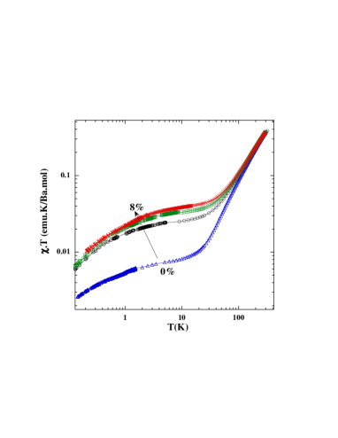
FIG. 14.: Fit of the experimental susceptibility in the temperature range [100 mK, 300 K]. We have shown $T\chi(T)$ versus T in a log-log plot. The susceptibility in the temperature range [100 mK, 1 K] has been fitted to an exponential term $C_{3}\exp{\left(-\frac{\Delta_{3}}{T}\right)}$.

The Haldane gap contribution (18) is extremely weak at low temperature. For instance one has $T\chi_{\rm Hald}(T)=1.2\times 10^{-6}$emu.K/Ba.mol if $T=10$ K.

Let us now improve the analysis of the low temperature susceptibility. We found that the experimental data in the temperature range [100 mK, 300 K] can be well described by a sum of two contributions (see Fig. 14):

$$T\chi(T)=T\chi_{\rm imp}(T)+T\chi_{\rm Hald}(T),$$ (17)

where $\chi_{\rm Hald}(T)$ is independent of doping concentration and describes the susceptibility associated with the formation of the Haldane gap at high temperature. $\chi_{\rm imp}(T)$ describes the low temperature susceptibility associated with the introduction of doping. Following a suggestion by Souletie et al. [34] we have attempted to represent $T\chi_{\rm Hald}(T)$ by the sum of two exponential contributions

$$T\chi_{\rm Hald}(T)=C_{1}\exp(-\frac{\Delta_{1}}{T})+C_{2}\exp(-\frac{\Delta_{2}}{T}),$$ (18)

rather than the usual activated behavior

$$\chi_{\rm Hald}(T)=AT^{-1/2}\exp{\left(-\Delta_{\rm Hald}/T\right)}$$ (19)

based on a quadratic expansion of the magnon dispersion relation around the minimum at $q=\pi$ [35]. The form (19) of the susceptibility is a good description of Haldane gap chains at temperatures smaller than $\Delta_{\rm Hald}/2$ [36, 37]. At higher temperatures, Souletie et al. [34] have found that (18) accounts extremely well for the results of exact diagonalizations and DMRG calculations on finite rings with an even number $N$ of spin-$1$ Heisenberg spins, extrapolated to the limit $N\rightarrow+\infty$. The agreement between these numerical calculations and Y₂BaNi_1-xZn_xO₅ is even quantitative since we found $\Delta_{2}/\Delta_{1}\simeq 3.8$ in Y₂BaNi_1-xZn_xO₅, instead of $\Delta_{2}/\Delta_{1}\simeq 3.86$ from the numerical calculations, and $C_{2}/C_{1}\simeq 0.25$ instead of $C_{2}/C_{1}\simeq 0.32$. Unlike Eq. (19), the expression (18) tends to the Curie law in the high temperature limit. It is particularly interesting that the expression (18) reaches a physically sound high temperature limit because this is in this limit that the Haldane term constitutes most of the magnetic signal. We took advantage of this situation to evaluate the Haldane gap term with the data above $1$ K and subtracted the corresponding contribution to extract an improved estimate of the impurity contribution.

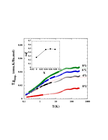
FIG. 15.: Temperature dependence of $T\chi_{\rm imp}(T)$. The fits correspond to (20). The insert show how $\gamma$ depends on the doping concentration $x$.

The difference $\chi_{\rm imp}(T)=\chi(T)-\chi_{\rm Hald}(T)$ can be interpreted as the susceptibility of the spin-$1/2$ moments generated by the Zn ions. We have shown on Fig. 15 the temperature dependence of $T\chi_{\rm imp}(T)$. We verified that the high temperature limit of $T\chi_{\rm imp}(T)$ corresponds approximately to a concentration $2x$ of spin-$1/2$ moments.

To describe the variation of $T\chi_{\rm imp}(T)$ we use two different expressions in the two temperature intervals [100 mK, 1 K] and [1 K, 300 K]. The impurity contribution shown in Fig. 15 has been fitted by a power law in the temperature range [1 K, 300 K] :

$$T\chi_{\rm imp}(T)=C_{\rm imp}\left(1+\frac{T_{\rm imp}}{T}\right)^{-\gamma},$$ (20)

where $C_{\rm imp}$ and $T_{\rm imp}$ are given in Table I, and $\gamma$ is shown on the insert in Fig. 15. We have found for the temperature range [100 mK, 1 K] that the experimental data are better described by a logarithmic temperature dependence (see Fig. 16):

$$T\chi_{\rm imp}(T)=A\log_{10}{\left({T\over T_{c}}\right)},$$ (21)

where $A$ and $T_{c}$ are given in Table I. Note that in this temperature range the contribution from the Haldane gap susceptibility (18) is negligible.

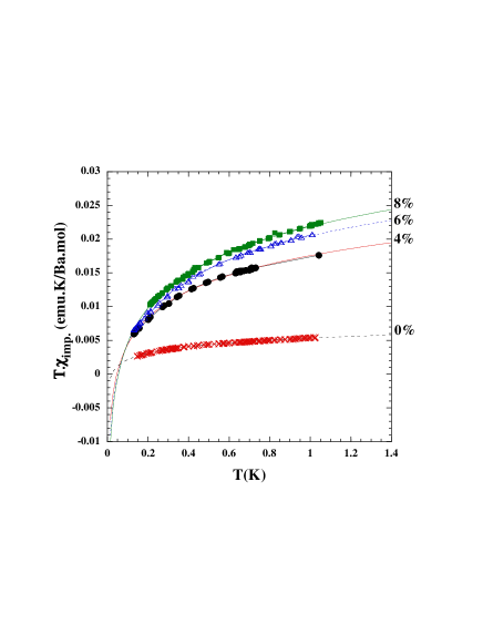
FIG. 16.: Fit of $T\chi_{\rm imp}(T)$ to the form (21) in the temperature range [100 mK, 1 K].

From the two fits given by (20) and (21) we deduce that $T\chi(T)$ tends to zero in the limit $T\rightarrow 0$. Regarding the discussion in section III B 2 we deduce that interchain interactions play an important role at low temperature. This validates the molecular field approach used in our theoretical description. Moreover the fit (20) suggests the existence of a finite Néel temperature $T_{c}$. We notice that

• The value of $T_{c}$ (see Table I) is too small to be probed directly in experiments.

• $T_{c}$ deduced from the fit (21) is one order of magnitude smaller than $\Theta$ deduced from the Curie-Weiss fit (16).

• $T_{c}$ increases with $x$, which is compatible with an interpretation in terms of a Néel temperature.

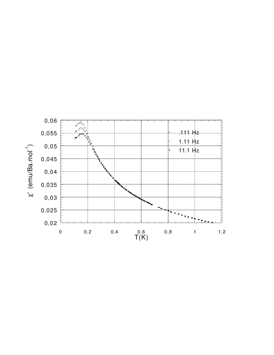
FIG. 17.: Temperature dependence of the ac-susceptibility $\chi^{\prime}(T)$ with $x=0.08$ for frequencies $f=0.11$ Hz, $f=1.1$ Hz, $f=11.1$ Hz. The temperature of the maximum of $\chi^{\prime}(T)$ is almost frequency-independent.

Finally we also performed ac-susceptibility measurements which are shown on Fig. 17 for three different frequencies. We have obtained a maximum in $\chi^{\prime}(T)$ at a temperature $T\simeq 160$ mK. The temperature of the maximum in the real part of the susceptibility is frequency-independent. This indicates that in spite of a slowing down of the dynamics at very low temperature, Y₂BaNi_1-xZn_xO₅ is not a spin glass at very low temperature. This may be contrasted with the hole doped compound Y_2-xCa_xBaNiO₅ [38] (with $0\leq x\leq 0.2$) in which a spin glass thermodynamic transition has been reported at $T_{g}=2-3$ K. The very low temperature ac-susceptibility of Y₂BaNi_1-xZn_xO₅ represented on Fig. 17 is reminiscent of the dc-susceptibility of the mean field model (see Fig. 5). We suggest that the very low temperature ac- and dc-susceptibilities (see Figs. 16 and 17) can be interpreted in terms of antiferromagnetic correlations at low temperature.

V Conclusion

To conclude, we have presented a detailed study of antiferromagnetic correlations in Y₂BaNi_1-xZn_xO₅. Based on the quantum chemistry calculation in Ref. [29], we have proposed that Y₂BaNi_1-xZn_xO₅ can be well described by a model in which interchain couplings are treated in mean field. The ground state of this model shows a coexistence between random dimers and antiferromagnetism. In the presence of the staggered molecular field, the product $T\chi(T)$ goes to zero in the limit of zero temperature.

We have presented very low susceptibility experiments and shown how to subtract from the total susceptibility the high energy contribution corresponding to the formation of the Haldane gap. The product $T\chi_{\rm imp}(T)$ tends to zero at low temperature. In view of the model, we conclude that this behavior is due to interchain correlations. At very low temperature the product $T\chi_{\rm imp}(T)$ has a logarithmic temperature dependence in the temperature interval [100 mK, 1 K]: $T\chi_{\rm imp}(T)\simeq A\log_{10}{(T/T_{c})}$. If we take for granted that this scaling is valid at lower temperatures we deduce the existence of a finite Néel transition temperature, which is in agreement with the assumption made in the mean field model. We have also obtained a maximum in the temperature dependence of the ac-susceptibility $\chi^{\prime}(T)$ which is an indication of the presence of antiferromagnetic correlations at very low temperature.

An important question left open is to clarify the behavior of 2D and 3D models and determine whether there is an antiferromagnetic phase transition at a finite temperature. Using a mean field model we have shown here that there is a coexistence between dimer formation (being due mainly to the even segments coupled antiferromagnetically) and antiferromagnetism (being due mainly to odd segments coupled ferromagnetically). If interchain interactions are very small, it is possible that singlets can be formed also among neighboring chains. These singlets would compete with 3D antiferromagnetism. An open question is to determine whether 3D antiferromagnetism is stable against dimer formation even with very small interchain interactions. Answering this question may clarify why $T_{c}$ (obtained from the fit (21) in the temperature range [100 mK, 1 K]) is one order of magnitude smaller than $\Theta$ (obtained from the Curie-Weiss fit (16) in the temperature range [1 K, 10 K]).

A Exact treatment of the two-spin model

1 Even segments

The Hamiltonian of even segments coupled antiferromagnetically reads

$${\cal H}=J(l){\bf S}_{1}.{\bf S}_{2}-h_{1}S_{1}^{z}+h_{2}S_{2}^{z},$$ (A1)

where we included a staggered molecular field $h_{s}=(h_{1}+h_{2})/2$ and a uniform field $h_{u}=(h_{1}-h_{2})/2$. The uniform field is used to calculate the uniform susceptibility. There are two eigenstates $|+,+\rangle$ and $|-,-\rangle$ with an energy $E_{|+,+\rangle}=J/4-h_{u}$, and $E_{|-,-\rangle}=J/4+h_{u}$. There are two other eigenstates $|\psi_{\epsilon}\rangle=x_{\epsilon}|+,-\rangle+y_{\epsilon}|-,+\rangle$ corresponding to $\epsilon=\pm 1$, with an energy

$$E_{\epsilon}=-\frac{J}{4}+\frac{\epsilon}{2}\sqrt{J^{2}+4h_{s}^{2}},$$

and

$$x_{\epsilon} = \sqrt{\frac{1}{2}-\epsilon\frac{h_{s}/J}{\sqrt{1+4h_{s}^{2}/J^{2}}}},$$ (A2)

$$y_{\epsilon} = \epsilon\sqrt{\frac{1}{2}+\epsilon\frac{h_{s}/J}{\sqrt{1+4h_{s}^{2}/J^{2}}}}.$$ (A3)

The magnetization is given by the thermal average

$$M(l,T)=\frac{e^{-\beta E_{|+,+\rangle}}-e^{-\beta E_{|-,-\rangle}}}{Z(T)},$$ (A4)

where the partition function is $Z(T)=\mbox{Tr}\exp{(-\beta{\cal H})}$, with $\beta=1/T$ the inverse temperature.

2 Odd segments

The odd segments are coupled ferromagnetically:

$${\cal H}=-|J(l)|{\bf S}_{1}.{\bf S}_{2}-h_{1}S_{1}^{z}-h_{2}S_{2}^{z},$$ (A5)

where $h_{1}=h_{2}=h_{s}+h_{u}$ in sublattice A and $h_{1}=h_{2}=-h_{s}+h_{u}$ in sublattice B. The solution of (A5) is straightforward.

B Renormalization of the two-spin model

We should distinguish between odd segments and even segments. We use the RG transformations given in Appendices C and D.

1 Even segments

We start from the Hamiltonian given by Eq. A1 in which the exchange is antiferromagnetic, and where we assume that there is no uniform magnetic field. There are three energy scales in the problem:

• The temperature $T$.

• The exchange gap $\Delta_{J}=J=\Delta\exp{(-l/\xi)}$.

• The staggered molecular field gap $\Delta_{h}=h_{s}$.

There are two relevant length scales:

• The thermal length $\xi_{T}$ for which $\Delta_{J}=T$. One has $\xi_{T}=\xi\ln{(\Delta/T)}$.

• The staggered molecular field length for which $\Delta_{J}=\Delta_{h}$. One has $\xi_{h}=\xi\ln{(\Delta/h_{s})}$.

We start the RG at high temperature, i.e. $T\sim\Delta$, and decrease the temperature until $\xi_{T}$ becomes equal to $\xi_{h}$. All the pairs of spins such that $l<\xi_{T}$ are frozen into dimers. Hence, the dimer order parameter $\varphi_{\rm dim}$ is given by

$$\varphi_{\rm dim}(T)=\int_{0}^{\xi_{T}}\frac{1}{2}{\cal P}(l)dl=\frac{1}{2}\left[1-\left(\frac{T}{\Delta}\right)^{x\xi}\right]\mbox{, where $T>h_{s}$}.$$

When the temperature becomes smaller than the staggered molecular field $h_{s}$, the spins that have not yet been decimated (i.e. having $l>\xi_{h}$) contribute to the antiferromagnetic order parameter:

$$\varphi_{\rm AF}(T)=\int_{\xi_{h}}^{+\infty}\frac{1}{2}{\cal P}(l)dl=\frac{1}{2}\left(\frac{h_{s}}{\Delta}\right)^{x\xi}\mbox{, where $T<h_{s}$}.$$

2 Odd segments

The odd segments are coupled ferromagnetically, with the Hamiltonian Eq. A5. At high temperature, the RG transforms the pairs of spin-$1/2$ moments having $l<\xi_{T}$ into spin-$1$ moments, having a renormalized staggered molecular field equal to $\tilde{h}_{s}=(h_{1}+h_{2})/2=h_{s}$. The density of spin-$1$ moment reads

$$\varphi_{1}(T)=\int_{0}^{\xi_{T}}\frac{1}{2}{\cal P}(l)dl=\frac{1}{2}\left[1-\left(\frac{T}{\Delta}\right)^{x\xi}\right]\mbox{, where $T>2h_{s}$}.$$

These spin-$1$ moments have a gap $\Delta_{h}=2h_{s}$. When $T=2h_{s}$, all of the spin-$1$ moments are frozen antiferromagnetically. The antiferromagnetic order parameter jumps from $\varphi_{\rm AF}(2h_{s}+0^{+})=0$ to

$$\varphi_{\rm AF}(2h_{s}-0^{+})=\frac{1}{2}\left[1-\left(\frac{2h_{s}}{\Delta}\right)^{x\xi}\right].$$

When $h_{s}<T<2h_{s}$, the pairs of spin-$1/2$ moments having a length $\xi_{2h_{s}}<l<\xi_{T}$ are transformed into spin-$1$ objects, which are immediately frozen antiferromagnetically. The antiferromagnetic order parameter is

$$\varphi_{\rm AF}(T)=\varphi_{\rm AF}(2h_{s}-0^{+})+\int_{\xi_{2h_{s}}}^{\xi_{T}}\frac{1}{2}{\cal P}(l)dl=\frac{1}{2}\left[1-\left(\frac{T}{\Delta}\right)^{x\xi}\right]\mbox{, where $h_{s}<T<2h_{s}$}.$$

When $T=h_{s}$, the survival spin-$1/2$ moments are directly frozen antiferromagnetically. The resulting antiferromagnetic order parameter is

$$\varphi_{\rm AF}(T)=\varphi_{\rm AF}(h_{s})+\int_{\xi_{h_{s}}}^{+\infty}\frac{1}{2}{\cal P}(l)dl=\frac{1}{2}\mbox{, where $T<h_{s}$}.$$

C RG transformations of ferromagnetic bonds

Let us consider the Hamiltonian

$${\cal H}=-J_{1,2}{\bf S}_{1}.{\bf S}_{2}-h_{1}S_{1}^{z}-h_{2}S_{2}^{z}.$$ (C1)

in which the spins $S_{1}$ and $S_{2}$ are coupled ferromagnetically. We replace the two spins $S_{1}$ and $S_{2}$ by an effective spin $S=S_{1}+S_{2}$ with a Hamiltonian ${\cal H}=-\tilde{h}S^{z}$, and need to calculate the renormalized field $\tilde{h}$. We use two different methods giving the same answer in the ferromagnetic case: (i) a semi-classical calculation using Holstein-Primakov bosons; (ii) a quantum mechanical calculation using Clebsch-Gordon coefficients.

1 Holstein-Primakov bosons

We replace the spin operators by their bosonic representation $S_{1}^{z}=S_{1}-a^{+}a$, $S_{1}^{+}=\sqrt{2S_{1}}a$, $S_{1}^{-}=\sqrt{2S_{1}}a^{+}$, and $S_{2}^{z}=S_{2}-b^{+}b$, $S_{2}^{+}=\sqrt{2S_{2}}b$, $S_{2}^{-}=\sqrt{2S_{2}}b^{+}$. The Hamiltonian Eq. C1 becomes

$${\cal H}=\left(-JS_{2}+h_{1}\right)a^{+}a+\left(-JS_{1}+h_{2}\right)b^{+}b+J\sqrt{S_{1}S_{2}}\left(ab^{+}+a^{+}b\right),$$ (C2)

where we discarded the classical energy contribution. The Hamiltonian Eq. C2 is diagonalized by the unitary transformation $a=c\cos{\theta}+d\sin{\theta}$, and $b=-c\sin{\theta}+d\cos{\theta}$, where

$$\tan{(2\theta)}=-\frac{2J\sqrt{S_{1}S_{2}}}{J(S_{1}-S_{2})+h_{1}-h_{2}}.$$

Expanding the low energy Hamiltonian to lowest order in $h_{1}$ and $h_{2}$ leads to

$$\tilde{h}(S_{1}+S_{2})=h_{1}S_{1}+h_{2}S_{2}.$$ (C3)

2 Clebsch-Gordan coefficients

We combine the two spins $S_{1}$ and $S_{2}$ to form a state of the type $|S_{1},S_{2}|S_{1}^{z},S_{2}^{z}\rangle$. The highest weight state is $|S,S\rangle=|S_{1},S_{2}|S_{1},S_{2}\rangle$, and we need to determine the states $|S,M\rangle$ to calculate $\langle S,M|-h_{1}S_{1}^{z}-h_{2}S_{2}^{z}|S,M\rangle$.

It is straightforward to show that

$$\langle S,S|-h_{1}S_{1}^{z}-h_{2}S_{2}^{z}|S,S\rangle=-h_{1}S_{1}-h_{2}S_{2}.$$ (C4)

Identifying this with $-\tilde{h}S$, we obtain the renormalized magnetic field Eq. C3. One can check that Eq. C3 is also valid for spin-$S$ states having lower values of $S^{z}$. For instance, one finds

$$|S,S-1\rangle=\sqrt{\frac{S_{1}}{S}}|S_{1},S-2|S_{1}-1,S_{2}\rangle+\sqrt{\frac{S_{2}}{S}}|S_{1},S_{2}|S_{1},S_{2}-1\rangle,$$

leading to

$$\langle S,S-1|-h_{1}S_{1}^{z}-h_{2}S_{2}^{z}|S,S-1\rangle=-\frac{S-1}{S}\left(h_{1}S_{1}+h_{2}S_{2}\right).$$ (C5)

Eq. C5 implies directly Eq. C3.

It can also be shown that

$$|S,S-2\rangle = \sqrt{\frac{S_{1}(2S_{1}-1)}{S(2S-1)}}|S_{1},S_{2}|S_{1}-1,S_{2}\rangle$$ (C6)

$$+ 2\sqrt{\frac{S_{1}S_{2}}{S(2S-1)}}|S_{1},S_{2}|S_{1}-1,S_{2}-1\rangle$$ (C7)

$$+ \sqrt{\frac{S_{2}(2S_{2}-1)}{S(2S-1)}}|S_{1},S_{2}|S_{1},S_{2}-2\rangle.$$ (C8)

We deduce

$$\langle S,S-2|-h_{1}S_{1}^{z}-h_{2}S_{2}^{z}|S,S-2\rangle=-\frac{S-2}{S}\left(h_{1}S_{1}+h_{2}S_{2}\right),$$ (C9)

leading again to Eq. C3.

We are lead to conjecture that

$$\langle S,M|-h_{1}S_{1}^{z}-h_{2}S_{2}^{z}|S,M\rangle=-\frac{M}{S}\left(h_{1}S_{1}+h_{2}S_{2}\right)$$ (C10)

for any value of $M$.

D RG transformations of antiferromagnetic bonds

Let us consider the Hamiltonian

$${\cal H}=J_{1,2}{\bf S}_{1}.{\bf S}_{2}-h_{1}S_{1}^{z}-h_{2}S_{2}^{z}$$ (D1)

in which the spins $S_{1}$ and $S_{2}$ are coupled antiferromagnetically. We assume that $S_{1}>S_{2}$ and look for the effective Hamiltonian under the form $-\tilde{h}S^{z}$, with $S=S_{1}-S_{2}$.

1 Holstein-Primakov bosons

To obtain the RG equation in the semiclassical limit, we represent the two spins by Holstein-Primokov bosons: $S_{1}^{z}=S_{1}-a^{+}a$, $S_{1}^{+}=\sqrt{2S_{1}}a$, $S_{1}^{-}=\sqrt{2S_{1}}a^{+}$, and $S_{2}^{z}=-S_{2}+b^{+}b$, $S_{2}^{+}=\sqrt{2S_{2}}b^{+}$, $S_{2}^{-}=\sqrt{2S_{2}}b$. The Hamiltonian Eq. D1 becomes

$${\cal H}=(JS_{2}+h_{1})a^{+}a+(JS_{1}-h_{2})b^{+}b+J\sqrt{S_{1}S_{2}}(ab+a^{+}b^{+}),$$ (D2)

where we retained only the quadratic contributions, and discarded the classical energy term. The bosonic Hamiltonian Eq. D2 is readily diagonalized by the Bogoliubov rotation $a=c\cosh{\theta}+d^{+}\sinh{\theta}$, with

$$\tanh{(2\theta)}=-\frac{2J\sqrt{S_{1}S_{2}}}{J(S_{1}+S_{2})+h_{1}-h_{2}}.$$

Expanding the low energy Hamiltonian to lowest order in $h_{1}$ and $h_{2}$ leads to

$$\tilde{h}(S_{1}-S_{2})=h_{1}S_{1}-h_{2}S_{2},$$ (D3)

which constitutes the classical renormalization equation. As we show in sections D 2 and D 3, the quantum renormalization equation does not coincide exactly with the classical equation.

2 Clebsch-Gordan coefficients: coupling of a spin-$s$ to a spin-$1/2$

Considering $S_{1}=s>1/2$ and $S_{2}=1/2$, we find

$$|s-1/2,M\rangle=\sqrt{\frac{s+M+1/2}{2s+1}}|s,1/2|M+1/2,-1/2\rangle-\sqrt{\frac{s-M+1/2}{2s+1}}|s,1/2|M-1/2,1/2\rangle,$$

from what we deduce $\langle s-1/2,M|-h_{1}S_{1}^{z}-h_{2}S_{2}^{z}|s-1/2,M\rangle=-\tilde{h}M$, with

$$\tilde{h}\left(s+\frac{1}{2}\right)=h_{1}(s+1)-\frac{1}{2}h_{2}.$$ (D4)

This RG equation is clearly not identical to Eq. D3.

3 Clebsch-Gordan coefficients: coupling of a spin-$s$ to a spin-$1$

Now let us consider $S_{1}=s>1$ and $S_{2}=1$. Using standard orthonormalization and recursion techniques, we obtain

$$|s-1,M\rangle = -\sqrt{\frac{(s-M)(s-M+1)}{2s(2s+1)}}|s,1|M-1,1\rangle$$ (D5)

$$+ \sqrt{\frac{(s+M)(s-M)}{s(2s+1)}}|s,1|M,0\rangle$$ (D6)

$$- \sqrt{\frac{(s+M+1)(s+M)}{2s(2s+1)}}|s,1|M+1,-1\rangle,$$ (D7)

form what we deduce $\langle s-1,M|-h_{1}S_{1}^{z}-h_{2}S_{2}^{z}|s-1,M\rangle=-\tilde{h}M,$ with the renormalized magnetic field

$$\tilde{h}s=h_{1}(s+1)-h_{2}.$$ (D8)

Comparing Eqs. D4 and Eq. D8, we are lead to conjecture that the general renormalization equation is

$$\tilde{h}(S_{1}-S_{2}+1)=h_{1}(S_{1}+1)-h_{2}S_{2}\mbox{ (with $S_{1}>S_{2}$)}.$$ (D9)

The quantum RG equation Eq. D9 does not coincide exactly with the classical one (see Eq. D3). Nevertheless, the large-$S$ limit of the quantum RG equation Eq. D9 does coincide with the classical equation Eq. D3.

REFERENCES

- [1] S.K. Ma, C. Dasgupta and C.K. Hu, Phys. Rev. Lett. 43, 1434 (1979); C. Dasgupta and S.K. Ma, Phys. Rev. B 22, 1305 (1980).
- [2] R.N. Bhatt and P.A. Lee, Phys. Rev. Lett. 48, 344 (1982).
- [3] D.S. Fisher, Phys. Rev. Lett. 69, 534 (1992); D.S. Fisher, Phys. Rev. B 50, 3799 (1994); D.S. Fisher, Phys. Rev. B 51, 6411 (1995).
- [4] R.A. Hyman, K. Yang, R.N. Bhatt, S.M. Girvin, Phys. Rev. Lett. 76, 839 (1996).
- [5] R.A. Hyman and K. Yang, Phys. Rev. Lett. 78, 1783 (1997).
- [6] C. Monthus, O. Golinelli, and Th. Jolicoeur, Phys. Rev. Lett. 79, 3254 (1997).
- [7] E. Westerberg, A. Furusaki, M. Sigrist, and P.A. Lee, Phys. Rev. B 55, 12578 (1997).
- [8] O. Motrunich, S.C. Mau, D.A. Huse, D.S. Fisher, Phys. Rev. B 61, 1160 (2000).
- [9] M. Hase, I. Terasaki and K. Uchinokura, Phys. Rev. Lett. 70, 3651 (1993); J.P. Pouget, L.P. Regnault, M. Ain, B. Hennion, J.P. Renard, P. Veillet, G. Dhalenne and A. Revcolevschi, Phys. Rev. Lett. 72, 4037 (1994).
- [10] J.-G. Lussier, S.M. Coad, D.F. McMorrow and D. McK Paul, J. Phys. Condens. Matter 7, L325 (1995).
- [11] P.E. Anderson, J.Z. Liu and R.N. Shelton, Phys. Rev. B 56 (1997), 11014.
- [12] M. Hase, N. Koide, K. Manabe, Y. Sasago, K. Uchinokura and A. Sawa, Physica B 215, 164 (1995).
- [13] M. Hase, K. Uchinokura, R.J. Birgeneau, K. Hirota and G. Shirane, J. Phys. Soc. Jpn. 65, 1392 (1996).
- [14] M.C. Martin, M. Hase, K. Hirota and G. Shirane, Phys. Rev. B 56, 3173 (1997).
- [15] T. Masuda, A. Fujioka, Y. Uchiyama, I. Tsukada, and K. Uchinokura, Phys. Rev. Lett. 80, 4566 (1998).
- [16] J.-P. Renard, K. Le Dang, P. Veillet, G. Dhalenne, A. Revcolevschi and L.P. Regnault, Europhys. Lett. 30, 475 (1995); L.P. Regnault, J.P. Renard, G. Dhalenne and A. Revcolevschi, Europhys. Lett. 32, 579 (1995).
- [17] K. Manabe, H. Ishimoto, N. Koide, Y. Sasago, and K. Uchinokura, Phys. Rev. B 58, R575 (1998).
- [18] F.D.M. Haldane, Phys. Lett. 93 a, 464 (1983); Phys. Rev. Lett. 50, 1153 (1983).
- [19] Y. Ichiyama, Y. Sasago, I. Tsukuda, K. Uchinokura, A. Zheludev, T. Hayashi, N. Miura, and P. Boni, Phys. Rev. Lett. 83, 632 (1999).
- [20] D.J. Buttrey, J.D. Sullivan, and A.L. Rheingold, J. Solid. State Chem. 88, 291 (1990).
- [21] B. Batlogg, S.W. Cheong, and L.W. Rupp Jr, Physica B 194-196, 173 (1994).
- [22] J.F. DiTusa, S.W. Cheong, J.H. Park, G. Aeppli, C. Broholm, and C.T. Chen, Phys. Rev. Lett. 73, 1857 (1994).
- [23] K. Kojima, A. Keren, L.P. Lee, G.M. Luke, B. Nachumi, W.D. Wu, Y.J. Uemura, K. Kiyono, S. Miyasaka, H. Takagi, and S. Uchida, Phys. Rev. Lett. 74, 3471 (1995).
- [24] C. Payen, E. Janod, K. Schoumacker, C.D. Batista, K. Hallberg, and A.A. Aligia, Phys. Rev. B 62, 2998 (2000).
- [25] H. Fukuyama, T. Tanimoto, and M. Saito, J. Phys. Soc. Jpn. 65, 1182, 1996.
- [26] M. Fabrizio and R. Mélin, Phys. Rev. Lett. 78, 3382 (1997); M. Fabrizio and R. Mélin, Phys. Rev. B 56, 5996 (1997); M. Fabrizio, R. Mélin, and J. Souletie, Eur. Phys. J. B 10, 607 (1999); R. Mélin, Eur. Phys. J. B 16, 261 (2000);
- [27] M. Fabrizio and R. Mélin, J. Phys.:Condens. Matter 9, 10429 (1997).
- [28] R. Mélin, Eur. Phys. J. B 18, 263 (2000).
- [29] C.D. Batista, A.A. Aligia, and J. Eroles, Europhys. Lett. 43, 71 (1998); C.D. Batista, Phys. Rev. B 58, 9248 (1998).
- [30] T. Kennedy, J. Phys.:Condens. Matter 2, 5737 (1990).
- [31] M. Hagiwara, K. Katsumata, I. Affleck, B.I. Halperin, and J.P. Renard, Phys. Rev. Lett. 65, 3181 (1990).
- [32] E. S. Sørensen and I. Affleck, Phys. Rev. B 51, 16115-16127 (1995)
- [33] S. Yamamoto and S. Miyashita, Phys. Rev. 50, 6277 (1994).
- [34] J. Souletie, M. Drillon, P. Rabu, and S.K. Pati, in preparation (2001).
- [35] L.P. Regnault, I.A. Zaliznyak, and S.V. Meskov, J. Phys.: Condens. Matter 5, L677 (1993).
- [36] M. Takigawa, T. Asano, Y. Ajiro, and M. Mekata, Phys. Rev. B 52, R13087 (1995).
- [37] Y.J. Kim, M. Greven, U.J. Wiese, and R.J. Birgeneau, Eur. Phys. J. B 4, 291 (1998).
- [38] E. Janod, C. Payen, F.X. Lannuzel, and K. Schoumacker, Phys. Rev. B 63, 212406 (2001).