Scaling in the growth of geographically subdivided populations: invariant patterns from a continent-wide biological survey

Abstract

We consider statistical patterns of variation in growth rates for over 400 species of breeding birds across North America surveyed from 1966 to 1998. We report two results. First, the standard deviation of population growth rates decays as a power-law function of total population size with an exponent $\beta=0.36\pm 0.02$. Second, the number of subpopulations, measured as the number of survey locations with non-zero counts, scales to the 3/4-power of total number of birds counted in a given species. We show how these patterns may be related, and discuss a simple stochastic growth model for a geographically subdivided population that formalizes the relationship. We also examine reasons that may explain why some species deviate from these scaling-laws.

1 Introduction

Perhaps one of the most intriguing patterns in ecology is Taylor’s law (Anderson et al., 1982; Soberón and Loevinsohn, 1987; Routledge and Swartz, 1991; Leps̆, 1993; Curnutt et al., 1996; Maurer, 1999). Taylor (1961) was the first to notice that when the mean $\langle S\rangle$ of a population survey is plotted versus its variance $\sigma^{2}(S)$, either in space or time, the relationship is typically a power-law with a fractional exponent

$$\sigma^{2}(S)\sim\langle S\rangle^{\gamma}\,.$$ (1)

Taylor was originally interested in the slope of the power-law relationship as a scale-free measure of spatial contagion or dispersion — values greater (less) than one indicate spatial clustering (over-dispersion). Later, Taylor used both spatial and temporal scaling as a basis for comparative studies of, in his words, “synoptic population dynamics” across taxonomic groups (Taylor and Woiwod, 1982; Taylor, 1984).

Taylor’s synoptic approach is, in many respects, a precursor to the recent development of “macroecology,” (Brown, 1995), a sub-discipline of ecology and biogeography (MacArthur and Wilson, 1967) that seeks to identify broad patterns in species’ abundance and distribution. Macroecology has largely focussed on static patterns, such as spatial relationships between abundance and environmental factors (Brown et al., 1995) and relationships between metabolic energy use and geographic distribution (Brown and Maurer, 1987). Thus, relatively few continental-scale macroecological studies (Maurer, 1994, 1999) have explored interactions between spatial distribution and population variability through time.

In this paper, we adopt Taylor’s synoptic approach and analyze one of the most comprehensive macroecological data sets available, the North American Breeding Bird Survey (Peterjohn, 1994). The data are estimates of local abundance (counts) for over 600 bird species recorded at 2–3 thousand sites (routes) across North America for the years 1966 to 1998. Unlike many previous macroecological studies, our focus is on linking geographic distribution to population dynamics. We report two new scaling laws, closely related to Taylor’s power-law, for these data: one relating variability of population time series to their mean, and another relating number of sites occupied to total population size. In addition, we show how these patterns may be related, and discuss a simple stochastic growth model for a geographically subdivided population that formalizes the relationship.

2 Scaling of species growth rates

Our goal is to understand temporal variation in abundance at the entire population level. We therefore compute time series of total counts for each species by summing over all routes surveyed in a given year (Fig, 1a). (We have previously analyzed these data at the individual route level, see Keitt and Stanley, 1998.) The aggregated time series should be relatively robust to observer errors inherent in the route-level data (Kendall et al., 1996) since random under-counts and over-counts will cancel in the summation. After performing a bias correction (see Appendix for details), the resulting time series are relatively free of systematic trends, particularly in the early years of the survey when the number of routes was increasing rapidly (compare dashed to solid lines in Fig. 1a).

We choose as our measure of the magnitude of time-series fluctuations, the logarithm of the ratio of successive counts,

$$g(t)\equiv\log\left(\frac{S(t+1)}{S(t)}\right)\,,$$ (2)

where $S(t)$ and $S(t+1)$ are the total number of birds of a given species counted in years $t$ and $t+1$, respectively. This measure has several nice properties. First, any multiplicative, time-independent sample bias cancels in the ratio. Second, the measure has a natural interpretation in terms of population demography since, in a closed population, $\exp[g(t)]\approx 1$ + (per capita birth rate - per capita death rate).

As shown in Fig. 1b, the standard deviation $\sigma(g)$ of population growth rates is strongly related to the average total population size. The relationship follows a power-law

$$\sigma(g)\sim\langle S\rangle^{-\beta}\,$$ (3)

for over four orders of magnitude in $\langle{S}\rangle$, the total count averaged across years. For these analyses, we are not interested in predicting a “dependent” variable from an “independent” variable. Rather, we are interested in modeling the functional form of the interdependence among variables. We therefore use major-axis regression (Sokal and Rohlf, 1995) to estimate model parameters. Major-axis regression is based on computing the leading eigenvector of the covariance matrix, and minimizes squared errors measured perpendicular to the trend line. We also restrict our analysis to non-zero time series of at least 25 years in length and with a minimum average total count of no fewer than 5 birds per year. Using major-axis regression with bootstrap precision estimates, we find $\beta=0.36\pm 0.02$. Taylor’s exponent (replicated across species) is simply $\gamma=2(1-\beta)=1.44\pm 0.04$.

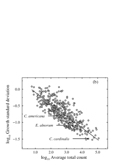
Figure 1: Scaling of ecological time series. (a) Time series of total counts for three species of birds (Northern Cardinal, Alder Flycatcher and Brown Creeper). Dashed lines show the uncorrected total number of birds counted in a given year. Solid lines are bias-corrected totals (see text for explanation). (b) Standard deviations of empirically observed population growth rates plotted against average annual total counts for 428 species of North American breeding birds. Results for the time series plotted in panel (a) are highlighted. Notice that the highlighted time series are less variable than other species in the data set with similar total population size.

We also study the scaling properties of population growth rates by examining changes in the distribution of growth rates with increasing population size, a technique familiar to statistical physicists. First, we separate the observed growth rates into three bins according to the total count $S(t)$ and then construct a histogram to estimate the conditional probabilities $p(g|S)$. The resulting distributions are roughly triangular in shape with the width depending on $S$ (Fig. 1a). (The triangular shape may result from summing over a large number of time series with different local variances, see Amaral et al., 1998). If the distributions are “self-similar” (i.e., exhibit scaling), then we should be able to identify a function $f$ that rescales the distributions so that they “collapse” onto each other (Stanley, 1971). We plot the scaled quantities:

$$\sigma(S)~{}p\left(\left.\frac{g}{\sigma(S)}\right|S\right)~{}~{}~{}{vs.}~{}~{}~{}\frac{g}{\sigma(S)}\,,$$ (4)

(Fig. 2a) and find that indeed the three curves do collapse onto each other (Fig. 2b), suggesting that $p(g|S)$ follows a universal scaling form

$$p(g|S)\sim\frac{1}{\sigma(S)}~{}~{}f\left(\frac{g}{\sigma(S)}\right)\,.$$ (5)

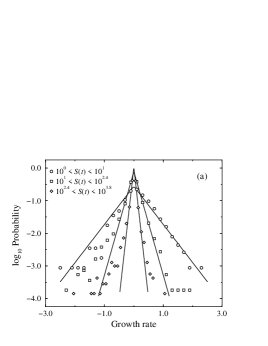
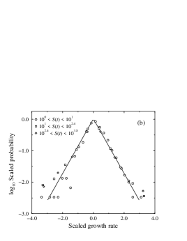
Figure 2: Distribution of growth rates for different population size classes. (a) Probability density $p(g|S)$ of the growth rate $g$ for all bird species in the North American Breeding Bird Survey database. The distribution represents all annual growth rates observed in the 31-year period 1966–1996. We show the data for three different bins of initial sizes. The solid lines are exponential fits to the empirical data close to the peak. The approximately triangular shape of the distribution may be the result of mixing Gaussians with different widths (Amaral et al., 1998). (b) Scaled probability density $p_{\mbox{\scriptsize scal}}\equiv\sigma p(g|S)$ as a function of the scaled growth rate $g_{\mbox{\scriptsize scal}}\equiv[g-\bar{g}]/\sigma$ for all species and years in the survey. The values were rescaled using the measured values of $\bar{g}$ and $\sigma$. All the data collapse upon the universal curve $p_{\mbox{\scriptsize scal}}=f(-|g_{\mbox{\scriptsize scal}}|)$.

These results are interesting for a number of reasons. In statistical physics, the presence of non-trivial scaling is usually taken to mean that the dynamics are largely governed by simple geometric properties of the system and do not depend strongly on detailed properties of the system subcomponents (Wilson, 1983). Thus, it is remarkable that we should find strong evidence for scaling across such a taxonomically and ecologically diverse set of species as found in the North American Breeding Bird Survey. These results suggest that the dynamics of North American Breeding Birds are unexpectedly “simple” and depend primarily on common patterns of internal population structure across species ranges, rather than details of individual species life-histories.

3 Spatial structure of subpopulations

Another reason the growth-scaling results are interesting is the large variability of highly abundant species. Imagine the null model that each population is subdivided into $n$ equally sized, independent subpopulations, and that the number of these subpopulations depends linearly on $S$. The expectation, according to the central limit theorem, is that the standard deviation in growth rates should decay as the -1/2 power of $S$. The observed decrease in fluctuations is considerably slower (i.e., $\beta<1/2$), such that highly abundant species are considerably more variable than expected under the null model.

To account for the increased variability for highly abundant species, we require that the number of subpopulations does not scale in a simple, linear fashion with increasing $S$, but instead takes the form:

$$n\sim S^{1-\alpha}\,,$$ (6)

with $\alpha\neq 0$. Values of $\alpha>0$ will be found, for example, when the “typical” size of the subpopulations also scales with total abundance, i.e., there is a positive relationship between regional and local abundance, a well documented pattern in macroecology (Gaston and Lawton, 1988; Gaston, 1996). The positive correlation between local and regional abundance results in fewer subpopulations for a given total population size as each subpopulation accounts for more individuals. Again appealing to our observation that, under the central limit theorem, $\sigma(g)\sim n^{-1/2}$, and in combination with equations (3) and (6), it is strait forward to show that for roughly equal-sized subpopulations, the estimated exponents must obey

$$\beta=\frac{1-\alpha}{2}\,.$$ (7)

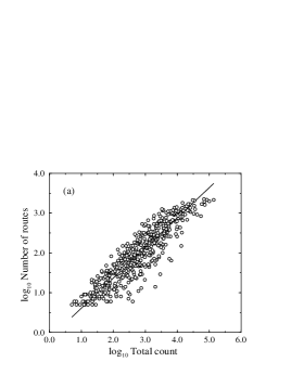
Figure 3: Statistical analysis of the number of routes populated by a given bird species. (a) Double logarithmic plot of the number of routes with non-zero counts $\tilde{n}(t)$ versus total number of birds counted $S(t)$ for each species observed in 1997. The bias correction applied to the time series in Fig. 1 is unnecessary in this case as all data come from a single year. The data for all species follow closely a straight line the log-log plot suggesting a power law dependence. From the slope of the line, we estimate $1-\alpha=0.75\pm 0.03$. (b) We perform a similar analysis for all 31 years in the database and plot the exponent estimates for each of the years. Our results show that the power law dependence remains remarkably stable during the 31 survey year, clustering around $\alpha=0.25$. Error bars are bootstrap 95% confidence intervals.

We do not have access to a precise estimate of the number of subpopulations for each species in the survey. However, we can use as a proxy the number of survey routes where a species had a non-zero count in a given year. To test the assertion in Eq. 7, we plot number of survey routes with non-zero counts $\tilde{n}(t)$ versus the (uncorrected) total count $S(t)$ for all bird species recorded in the survey in 1997, excluding species seen at fewer than 5 routes or with fewer than 5 total individuals counted. The data follow closely the power law dependence predicted by Eq. (6) with an exponent $\alpha=0.25\pm 0.03$, again using major-axis regression with bootstrap precision estimates (Fig. 3a). Remarkably, the estimate of $\alpha$ predicts a value of $\beta=0.38\pm 0.02$, very close to the estimate ($\beta=0.36\pm 0.02$) obtained by measuring the standard deviation in growth rates directly (Fig. 1b). Even more striking is the consistency of our estimate of $\alpha$ across years, despite large changes in the number and spatial distribution of sampling locations through time (Fig. 3b). These results directly imply that average local abundance $\langle s\rangle=S(t)/\tilde{n}(t)$, scales with total (regional) abundance according to $\langle s\rangle\sim S(t)^{\alpha}$.

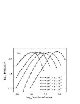
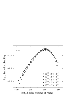
Figure 4: Statistical analysis of the number of routes populated by a given bird species. (a) Conditional probability density function $\rho(\tilde{n}|S)$ of finding $\tilde{n}$ non-zero count routes for a bird species with $S$ total counts. To improve the statistics, we partition the bird species into four groups according to size. (b) To illustrate the scaling relation (8), we plot the scaled probability density $S^{1-\alpha}~{}\rho(\tilde{n}/S^{1-\alpha}|S)$ versus the scaled number of non-zero routes $\tilde{n}/S^{1-\alpha}$, combining data from all years. In agreement with (8), we find that the scaled data fall onto a single curve.

We can gain further insight into the organization of a species population in different routes by considering how the distribution of number of routes with non-zero counts depends on total counts. That is, we may quantify the organization of the subpopulations through the conditional probability density $\rho(\tilde{n}|S)$, which measures the probability to find a bird species with S total counts having non-zero counts in $\tilde{n}$ distinct routes. Fig. 3 suggests that $\rho(\tilde{n}|S)$ will have a peak that increases as a power law with $S$. As shown in Fig. 4a this is indeed the case. If the data exhibit scaling, we should be able to identify a universal scaling function $h$ such that

$$\rho(\tilde{n}|S)\sim\frac{1}{S^{\alpha}}~{}~{}h\left(\frac{\tilde{n}}{S^{\alpha}}\right)\,,$$ (8)

We test the scaling hypothesis in Eq. (8) by plotting the scaled variables:

$$S^{\alpha}~{}\rho\left(\left.\frac{\tilde{n}}{S^{\alpha}}\right|S\right)~{}~{}~{}{vs.}~{}~{}~{}\frac{\tilde{n}}{S^{\alpha}}\,.$$ (9)

Fig. 4b shows that all curves collapse onto a single curve, which yields the scaling function $h(u)$.

4 Discussion

Our analysis differs from Taylor’s original studies  (Taylor, 1961; Taylor and Woiwod, 1982; Taylor, 1984) in an important way. Taylor was interested in comparative analysis and so calculated a separate exponent for each species. He did this by analyzing multiple samples, replicated across time or space, for each species. Here, we calculate exponents replicating across species. One advantage of this approach is that we analyze the time series of total counts, summed over the entire survey. These total counts are considerably more robust estimates of abundance than local counts taken at individual routes.

Another advantage of analyzing scaling across species is that is allows us separate general patterns or “laws” that are invariant across taxonomic groups from general rules that may explain deviations from these laws. Our reasoning is that when the physical dimensions of a problem, such as energy or material flows, or spatial population structure, predominate, we should observe scaling laws that do not depend strongly on the biological differences among species, but that species-specific differences should appear as residual variation after the common scaling laws are factored out. That so many species fall along a single scaling relationship describing variability as a function of population size (Fig. 1–2) suggests that there may be universal features to the way in which North American breeding bird populations are subdivided spatially. We find exactly these features in the invariant, 3/4-power scaling of number of occupied survey routes versus total population size (Fig. 3–4).

However, not all of the variability in the data is accounted for by these scaling laws. For example, species with average total counts of approximately 250 individuals exhibit more than two orders of magnitude range in growth rate standard deviation (Fig. 1b). We believe that this residual variation does reflect important aspects of the ecology of individual species. There is a strong correlation between the residuals in Fig. 1b and the area of the corresponding species ranges, measure in terms of the average number of non-zero routes (T. Keitt, unpublished results). A likely explanation for this pattern is that fluctuations in the abundances of broadly distributed species will tend to average out spatially because different regions are influenced by geographically distinct climate regimes. Thus, it appears that species whose life histories tend to produce strongly aggregated distributions (i.e., species that are locally common, but regionally rare) are the ones that fluctuate the most relative to their total abundance. Species that have broad spatial distributions (i.e., locally rare, but regionally common) are therefore expected to fluctuate less than similar species with more restricted geographic ranges.

Ranking species in terms of their residual deviation from the growth-scale law (Fig. 1b) supports our hypothesis that locally common, but regionally rare species fluctuate more than expected, and vise versa. Large positive residuals correspond to species with restricted geographic ranges, such as Golden-cheeked Warbler (Dendroica chrysoparia; 2.5 times more variable), species that are habitat specialists and nest in large colonies, such as Tricolored Blackbird (Agelaius tricolor; 13.7 times more variable), species that breed in large groups called “leks”, such as Greater Prairie Chicken (Tympanuchus cupido; 3 times more variable), and species that show strong local migration patterns in response to changes in resource availability, such as White-winged Crossbill (Loxia leucoptera, 3.5 times more variable) and Red Crossbill (Loxia pytyopsittacus; 3.7 times more variable). Species that show low variability in relation to the scaling-law are typically solitary, territorial breeders such as Yellow-throated Warbler (Dendroica dominica; 2.8 times less variable), Prairie Falcon (Falco mexicanus; 2.6 times less variable), Swamp Sparrow (Melospiza georgiana; 2.5 times less variable), Kentucky Warbler (Oporornis formosus; 2.4 times less variable), and Chuck-will’s-widow (Caprimulgus carolinensis; 2.3 times less variable). The important point is that had we started from a purely autecological standpoint and ignored the important physical dimensions of the problem (e.g., structure of geographic ranges), we could easily have missed key pattern in terms of deviations from general scaling laws.

We should however mention several caveats. We do not as of yet know whether our results can be generalized to include other, non-avain taxonomic groups, or to other continents and climate regimes. Also, despite our use of highly aggregated, and therefore more robust time series, we suspect that there remain sources of variation in our analysis unrelated to actual population fluctuations. One vexing problem is repeated local migration between sampled and unsampled locations (we call this “sloshing”). Even if there is no variation in the true abundance across years, sloshing will lead to a given individual being counted in some years and not others, leading to measurement errors in the time series. We suspect this effect is not a significant component of variation in most of our time series, but may be substantial in a few cases. (Sloshing may contribute to the extreme variability of Tricolored Blackbird, for example.) Additional data, such as mark-recapture, may be need to resolve this issue.

There are two additional mechanisms related to our model for geographically subdivided populations that we have not discussed. We have shown how a non-linear dependency of the number of subpopulations versus total population size may explain the observed deviation from 1/2-power scaling of population fluctuations. Our basic hypothesis depends on the average local abundance scaling with total abundance in independently fluctuating subpopulations of roughly equal size. However, there are other patterns that may influence the “effective” number of independently fluctuating subpopulations and thus partially amount for the observed exponent in the growth-scaling law. First, large spatial variation in local abundance (Brown et al., 1995) could cause wide-spread species to fluctuate with greater magnitude than if all subpopulations have the same local abundance, since most of the variation would be driven by a few, high abundance sites. Second, strong spatial autocorrelation in population growth increments or “spatial synchrony” among fluctuating subpopulations (Grenfell et al., 1998; Bjørnstad et al., 1999; Kendall et al., 2000; Lundberg et al., 2000) may also cause a reduction in the effective number of independent subpopulations, and thus account for the increased magnitude of fluctuation in broadly distributed species. Temporal autocorrelation may act similarly to increase or decrease variability relative to our model. The consequences of these mechanisms need further exploration.

A surprising result of our analysis is the, to our knowledge, previously unreported 3/4-power scaling of spatial distribution as a function of total population size (Fig. 3). This result is closely related to, but not the same as, the “Distribution-Abundance” curve of Hanski and Gyllenberg (1997) that describes the fraction of regional habitats occupied as a function of average local abundance. We do not as of yet have an explanation for why the exponent should take this particular value, nor why it is so consistent through years. Recently, there has been considerable interest in explanations for the apparent 3/4-power scaling law relating body mass to metabolic output (Enquist et al., 1998; West et al., 1999; Dodds et al., 2001; Niklas and Enquist, 2001). One explanation posited to explain 3/4-power scaling is optimal structuring of a fractal transport network, such as the vascular system of plants and animals (West et al., 1999). This suggests an interesting hypothesis to explain 3/4-power scaling in our analysis: if the geographic ranges of species are subdivided in according to a particular fractal pattern, perhaps because of the fractal nature of the physical environment (e.g., Rinaldo et al., 1995), then it might lead to our observed scaling laws. Testing this hypothesis will require additional study.

It is interesting to note that our results are in striking qualitative agreement with similar studies from a broad range of social systems, ranging from growth of companies in the U.S. economy to the GDP of countries (Stanley et al., 1996; Lee et al., 1998; Plerou et al., 1999), suggesting that our simple model of growth may apply quite broadly (Amaral et al., 1998). Our observation that more “specialized” birds (in terms of smaller number of subpopulations) fluctuate more in total number than those that average fluctuations over many subpopulations may have an interesting parallel in social organizations: those that specialize on a few economic activities, e.g., countries with a single export product, may fluctuate considerably more than similarly sized organization with diverse economic activities, e.g., countries that produce a range of products. Putting all of one’s eggs in a single basket, as the saying goes, some times leads to catastrophes, and, it appears, greater variability as well.

5 Acknowledgements

T. Keitt thanks the Santa Fe Institute and the National Center for Ecological Analysis and Synthesis for support during the initial phase of this research. This research was made possible by the efforts by thousands of U.S. and Canadian BBS participants in the field, as well as, USGS and CWS researchers and managers.

Appendix: Corrections applied to time series

Let $s_{tuv}$ be the number of birds of species $u$ counted at route $v$ in year $t$. The raw total counts $R_{tu}=\sum_{v}^{N_{t}}s_{tuv}$ contain information about the abundance of species $u$ in year $t$ as well as information about the number $N_{t}$ and distribution of routes surveyed in year $t$. The goal is to remove the bias in the counts $R_{tu}$ introduced by variation in the number and distribution of survey routes through time. We do this by replacing each count $s_{tuv}$ for a given species at a given route with the time average $\mu_{uv}=T_{v}^{-1}\sum_{t}s_{tuv}$ for that route and species, where $T_{v}$ is the number of years that route $v$ was surveyed. We then construct new, surrogate time series $M_{tu}=\sum_{v}^{N_{t}}\mu_{uv}$ whose variation only reflects changes in the number and distribution of survey routes through time (because the same $\mu_{uv}$ is used in each year), and not any real change abundance. We can then generate a bias corrected time series by subtracting these new time series from the raw totals:

$$S_{tu}=R_{tu}-M_{tu}+\bar{M}_{u}$$ (10)

where $\bar{M}_{u}$ is the time average of $M_{tu}$ for species $u$. The advantage of this approach is that survey routes added or removed outside a species range will not influence the corrected total, because these routes will have $\mu_{uv}=0$.

References

- Amaral et al. (1998) Amaral, L. A. N., Buldyrev, S. V., Havlin, S., Salinger, M. A., and Stanley, H. E. (1998). Power law scaling for a system of interacting units with complex internal structure. Physical Review Letters, 80, 1385–1388.
- Anderson et al. (1982) Anderson, R. M., Gordon, D. M., Crawley, M. J., and Hassel, M. P. (1982). Variability in the abudance of animal and plant species. Nature, 296, 245–248.
- Bjørnstad et al. (1999) Bjørnstad, O. N., Ims, R. A., and Lambin, X. (1999). Spatial population dynamics: Analyzing patterns and processes of spatial synchrony. Trends in Ecology and Evolution, 14(11), 427–432.
- Brown (1995) Brown, J. H. (1995). Macroecology. The University of Chicago Press, Chicago.
- Brown and Maurer (1987) Brown, J. H. and Maurer, B. A. (1987). Evolution of species assemblages: Effects of energetic constraints and species dynamics on the diversification of the North American avifauna. The American Naturalist, 130(1), 1–17.
- Brown et al. (1995) Brown, J. H., Mehlman, D. W., and Stevens, G. C. (1995). Spatial variation in abundance. Ecology, 76(7), 2028–2043.
- Curnutt et al. (1996) Curnutt, J. L., Pimm, S. L., and Maurer, B. A. (1996). Population variablity of sparrows in space and time. OIKOS, 76, 131–144.
- Dodds et al. (2001) Dodds, P. S., Rothman, D. H., and Weitz, J. S. (2001). Re-examination of the ”3/4-law” of metabolism. Journal of Theoretical Biology, 209, 9–27.
- Enquist et al. (1998) Enquist, B. J., Brown, J. H., and West, G. B. (1998). Allometric scaling of plant energetics and population density. Nature, 395, 163–165.
- Gaston (1996) Gaston, K. J. (1996). Species-range-size distributions: Patterns, mechanisms and implications. TREE, 11, 197–201.
- Gaston and Lawton (1988) Gaston, K. J. and Lawton, J. H. (1988). Patterns in the distribution and abundance of insect populations. Nature, 331, 709–712.
- Grenfell et al. (1998) Grenfell, B. T., Wilson, K., Finkenstädt, B. F., Coulson, T. N., Murray, S., Albon, S. D., Pemberton, J. M., Clutton-Brock, T. H., and Crawley, M. J. (1998). Noise and determinism in sychronized sheep dynamics. Nature, 394, 674–677.
- Hanski and Gyllenberg (1997) Hanski, I. and Gyllenberg, M. (1997). Uniting two general patterns in the distribution of species. Science, 275, 397–400.
- Keitt and Stanley (1998) Keitt, T. H. and Stanley, H. E. (1998). Dynamics of North American breeding bird populations. Nature, 393, 257–260.
- Kendall et al. (2000) Kendall, B. E., Bjørnstad, O. N., Bascompte, J., Keitt, T. H., and Fagan, W. F. (2000). Dispersal, environmental correlation, and spatial synchrony in population dynamics. The American Naturalist, 155, 628–636.
- Kendall et al. (1996) Kendall, W. L., Peterjohn, B. G., and Sauer, J. R. (1996). First-time observer effect in the North American breeding bird survey. The Auk, 113(4), 823–829.
- Lee et al. (1998) Lee, Y., Amaral, L. A. N., Canning, D., Meyer, M., and Stanley, H. E. (1998). —. Physical Review Letters, 81, 3275–.
- Leps̆ (1993) Leps̆, J. (1993). Talor’s power law and the measurement of variation in the size of populations in space and time. OIKOS, 68(2), 349–356.
- Lundberg et al. (2000) Lundberg, P., Ranta, E., Ripa, J., and Kaitala, V. (2000). Population variability in space and time. Trends in Ecology and Evolution, 15(11), 460–464.
- MacArthur and Wilson (1967) MacArthur, R. H. and Wilson, E. O. (1967). Island Biogeography. Princeton University Press, Princeton, New Jersey.
- Maurer (1994) Maurer, B. A. (1994). Geographical Population Analysis: Tools for the Analysis of Biodiversity. Blackwell Scientific Publications, Oxford.
- Maurer (1999) Maurer, B. A. (1999). Untangling Ecological Complexity: The Macroscopic Perspective. The University of Chicago Press.
- Niklas and Enquist (2001) Niklas, K. J. and Enquist, B. J. (2001). Invariant scaling relationships for interspecific plant biomass production rates and body size. Proceeding of the National Academy of Sciences, 98, 2922–2927.
- Peterjohn (1994) Peterjohn, B. G. (1994). The North American breeding bird survey. Birding, Journal of the American Birding Assocation, 26(6).
- Plerou et al. (1999) Plerou, V., Amaral, L. A. N., Gopikrishnan, P., Meyer, M., and Stanley, H. E. (1999). Similarities between the growth dynamics of university research and of competitive economic activities. Nature, 400, 433–437.
- Rinaldo et al. (1995) Rinaldo, A., Dietrich, W. E., Rigon, R., Vogel, G. K., and Rodrigueziturbe, I. (1995). Geomorphological signatures of varying climate. Nature, 374, 632–635.
- Routledge and Swartz (1991) Routledge, R. D. and Swartz, T. B. (1991). Taylor’s power law re-examined. OIKOS, 60(1), 107–112.
- Soberón and Loevinsohn (1987) Soberón, J. and Loevinsohn, M. (1987). Patterns of variations in the number of animal populations and the biological foundations of Taylor’s law of the mean. OIKOS, 48(3), 249–252.
- Sokal and Rohlf (1995) Sokal, R. R. and Rohlf, F. J. (1995). Biometry; the principles and practice of statistics in biological research. W. H. Freeman, San Francisco, 3 edition.
- Stanley (1971) Stanley, H. E. (1971). Introduction to Phase Transitions and Critical Phenomena. Oxford University Press, Oxford.
- Stanley et al. (1996) Stanley, M. H. R., Amaral, L. A. N., Buldyrev, S. V., Havlin, S., Leschhorn, H., Maass, P., Salinger, M. A., and Stanley, H. E. (1996). Scaling behavior in the growth of companies. Nature, 379, 804–806.
- Taylor (1961) Taylor, L. R. (1961). Aggregation, variance and the mean. Nature, 189, 732–735.
- Taylor (1984) Taylor, L. R. (1984). Synoptic dynamics, migration and the Rothhamsted insect survey. Journal of Animal Ecology, 55, 1–38.
- Taylor and Woiwod (1982) Taylor, L. R. and Woiwod, I. P. (1982). Comparative synoptic dynamics. I. Relationships between inter- and intra-specific spatial and temporal variance/mean population parameters. Journal of Animal Ecology, 51, 879–906.
- West et al. (1999) West, G. B., Brown, J. H., and Enquist, B. J. (1999). The fourth dimension of life: Fractal geometry and allometric scaling of organisms. Science, 284(5420), 1677–1679.
- Wilson (1983) Wilson, K. G. (1983). The renormalization group and critical phenomena. Review of Modern Physics, 55, 583–600.