PHYSICAL REVIEW B Volume 65, Number 19-20 15 May 2002 Activation energy in a quantum Hall ferromagnet and non-Hartree-Fock Skyrmions

I. INTRODUCTION

 

Up to now, in two-dimensional (2D) electron gas (EG) the quantum Hall effect (QHE) at the Landau-level (LL) filling factor of $\nu=1$, has attracted much theoretical[1, 2, 3, 4, 5, 6, 7, 8] and experimental[9, 10, 11, 12, 13, 14, 15, 16] attention. The interest is explained by the fact that in this regime at vanishing (or considerably reduced) Zeeman coupling peculiar Fermionic excitations exist: namely, these are skyrmions, characterized by a large spin, $|\delta S_{z}|\gg 1$, and by a topological invariant (or topological charge) in terms of a field theory of the classical 2D ferromagnet.[17, 18] The first mapping of the spin-polarized quantum Hall system to an appropriate nonlinear $O(3)$ model, of the 2D ferromagnet, was used in the work of Sondhi et al  [1] to calculate the skyrmion energy. Within the context of the phenomenological approach employed the creation gap (i.e, the combined energy of a skyrmion-antiskyrmion pair) was found in the ideal 2D case to be exactly equal to half the gap in creating an electron-hole pair. (The latter is considered as an extreme case of a spin exciton with $\delta S_{z}=-1$.) Due to this result, at once the theory became by factor of 2 closer to the data found experimentally for the QHE activation gap. However, this and all later calculations, still remain in striking discrepancy with measurements. There is growing experimental evidence [13, 14, 15, 16] that at zero Landé factor, the energy required for activation of a dissipative current in a quantum Hall ferromagnet, is approximately a factor of 0.1 smaller than the calculated skyrmion-activation energy (the latter is one-half the creation gap).

Justification for the application of the nonlinear $O(3)$ model to the quantum Hall ferromagnet (QHF) is confirmed by a microscopical theory based on the Hartree-Fock (HF) Hamiltonian for the Coulomb interaction and on the approximation of wave functions projected (WFP) onto a single LL.[4, 5, 6] In these works, the energy of isolated skyrmionic excitations is recalculated and the minimum creation gap becomes the same as in Ref. [1]. Another approach, developed by Iordanskii et al  [7] does not use the approximation of WFP. The authors describe a skyrmion excitation as a smooth nonuniform rotation in real three-dimensional spin space. Due to the fact that the Coulomb Hamiltonian is invariant with respect to such a rotation, this approach has an evident advantage. The authors calculate the energy of skyrmionic excitations with the help of the perturbation theory technique. This theory uses for a bare Green function (GF) the appropriate mean-field one-electron GF. In doing so, the HF approximation is employed and the results (after a small correction[8]) turn out to be in agreement with earlier results.[4, 5] (See below in the Appendix II.) Naturally, any effects of LL mixing are neglected there, and the results reported in Refs. [4, 5, 6, 7, 8], as well as in Ref. [1], represent the energy of skyrmions only in terms of a linear approximation of the Coulomb interaction; i.e. only in the framework of the first-order approximation in the parameter $r_{\mbox{C}}$ which is supposed to be small.

In our work the energy of skyrmions is calculated analytically with the help of the modified perturbation-theory technique. This technique is based on the excitonic representation (ER) which is suitable when a 2D EG is in a dielectric state, i.e. in the absence of free electrons and holes (see Refs. [19, 20, 21, 22, 23, 24, 25, 26]). Neither the HF nor WFP approximations are used. As in the case of Ref. [7], a skyrmion excitation is considered as a rotation in 3D space:

$${\vec{\psi}}({\bf r})={\hat{U}}({\bf r}){\vec{\chi}}({\bf r}),\quad{\bf r}=(x,y)\,.$$

Here ${\vec{\psi}}$ is a spinor given in the stationary coordinate system and ${\vec{\chi}}$ is a new spinor in the local coordinate system accompanying this rotation. The rotation matrix of ${\hat{U}}({\bf r})\quad$ ($U^{{\dagger}}U=1$) is parametrized by three Eulerian angles.[27] In the zero approximation in terms of ${\hat{U}}({\bf r})$ gradients[28], we get ${\vec{\chi}}\propto{1\choose 0}$. Generally, in the limit of a vanishing Landé $g$ factor, the results obtained may be presented as an exact expansion in terms of the parameter $r_{\mbox{C}}$. Virtually two first terms of this expansion have been calculated exactly.

As a first step, we ignore the Coulomb-interaction processes responsible for any decay of a one-exciton state due to the transformation into two-exciton states. Specifically, the part of the Coulomb Hamiltonian kept involves: first, the terms responsible for the direct Coulomb interaction without any LL mixing; second, the terms providing the shift of the exchange self-energy if an electron is transferred from one LL to another; and finally, the random-phase-approximation terms in which an exciton transforms into another one at a different point of conjugate space, but with the same spin state and the same cyclotron part of energy. In other words, such a reduced Hamiltomian corresponds to a proper mean-field approach formulated in relation to excitons, but not to a quasiparticle excitation (as it would be in the case of the HF approximation). This Hamiltonian is “excitonically diagonalized” (ED) and all one-exciton states (spin waves, magnetoplasmons and spin-flip magnetoplasmons) present a full basic set for its exact diagonalization.[29] The main idea of the present work is to employ a basic set of one-exciton states for the perturbation-theory formalism, instead of the basic set of one-particle states. If we restrict our study to the terms of the excitonically diagonalized Hamiltonian (EDH), then the energies of skyrmion excitations may be found in a very simple way for any magnitude of $r_{\mbox{C}}$. In the QHF, at $\nu=1$, and in the strict 2D limit we obtain the energy of the hole-like skyrmion $E_{\mbox{ED}+}=\frac{3}{4}\sqrt{\pi/2}r_{\mbox{C}}\hbar\omega_{c}$, and the energy of the electron-like anti-skyrmion $E_{\mbox{ED}-}=\Delta_{\mbox{ED}}-E_{\mbox{ED}+}$, where $\Delta_{\mbox{ED}}$ is the skyrmion creation gap:

$$\Delta_{\mbox{ED}}=\hbar\omega_{c}{\sqrt{\frac{\pi}{2}}r_{\mbox{C}}}\left/\left({2+\sqrt{\frac{\pi}{2}}r_{\mbox{C}}}\right)\right.$$

$$\equiv\frac{\hbar\omega_{c}(e^{2}/\varepsilon l_{B})}{\sqrt{8/\pi}\hbar\omega_{c}+e^{2}/\varepsilon l_{B}}\,.$$

In the EDH model the gap thereby is determined by the smallest value among the cyclotron and Coulomb energies. At the same time, the EDH approach gives exact results of the first order in the expansion in terms of $r_{\mbox{C}}$. In the limit of $r_{\mbox{C}}\to 0$ they are curiously in agreement with the results obtained within the HF and WFP approximations[4, 5] when the gap is $\frac{1}{2}\sqrt{\pi/2}r_{\mbox{C}}\hbar\omega_{c}$. This coincidence of the $r_{\mbox{C}}\!\to 0\!$ results seems to be connected only with a special symmetry of the system studied (see the discussion in Appendix II).

The rest of the terms of the total Coulomb Hamiltonian are responsible for other various LL mixing processes and provide additional corrections of the second and higher degrees of $r_{\mbox{C}}$. The calculation carried out in Sec. IV (at $\nu=1$) yields the exact second-order corrections $E^{(2)}_{+}=-0.008r_{\mbox{C}}^{2}\hbar\omega_{c}$ for the skyrmion and $\Delta E^{(2)}=-0.382r_{\mbox{C}}^{2}\hbar\omega_{c}$ for the creation gap. These corrections are independent of the magnetic field.

It is interesting that in the opposite case, when $r_{\mbox{C}}\gg 1$, the Coulomb terms not involved in the EDH give again only small corrections of the order of $\hbar\omega_{c}/r_{\mbox{C}}$ to the fermion creation gap (see the end of Sec. IV). Therefore, if we formally consider the $r_{\mbox{C}}\to\infty$ limit (by keeping the magnetic field constant we can study the $\varepsilon\to 0$ limit), then for an ideally clean sample the EDH formula (1.2) represents also the correct result $\Delta_{\mbox{ED}}\to\hbar\omega_{c}$. This has to take place for skyrmions which are characterized by a smooth spatial function on the length scale of $l_{B}$. The reasoning explaining this outcome may be as follows. Indeed, at a fixed $\nu=1$ the parameter $r_{\mbox{C}}$ has one more meaning: it is the average inter-particle separation in units of the effective Bohr radius $a_{B}=\hbar^{2}\varepsilon/m_{e}^{*}e^{2}$. When $r_{\mbox{C}}\gg 1$, the average Coulomb interaction is weak as compared to the effective Bohr atomic energy $E_{B}=m_{e}^{*}e^{4}/\hbar^{2}\varepsilon^{2}$, and it ceases being responsible for the gap determined by lowest-energy spatial excitations. [30] However, in accordance with the Kohn theorem, [31] the cyclotron frequency remains always a relevant parameter of the clean system. If $r_{\mbox{C}}\gg 1$, then $\hbar\omega_{c}$ is the smallest quantity in the energy scale, $\hbar\omega_{c}\ll e^{2}/\varepsilon l_{B}\ll E_{B}$, and the fermionic gap has to approach $\hbar\omega_{c}$ or zero. Since the $\nu=1$ condition seems always to provide an insulator phase of the system studied, the result $\Delta\to\hbar\omega_{c}$ is natural in the considered limit.

Of course, these simple speculations ignore a disorder which turns out to be the main factor, and it really governs the spectrum of the system just at $r_{\mbox{C}}\gg 1$. This case is practically realized at comparatively low magnetic field. Then the picture at large $r_{\mbox{C}}$ is determined by the competition between disorder and magnetic field or between disorder and interaction, and it turns out to be rather diverse (e.g. see Refs. [32, 33] and the works cited therein).

Meanwhile, in the clean limit just the situation when $r_{\mbox{C}}\sim 1$ becomes experimentally relevant. Then our calculations within the EDH framework (Sec. III) as well as beyond of it (Sec. IV) demonstrate that the skyrmion-creation gap is substantially reduced in comparison with the HF and WFP calculations. In extrapolating to the region $r_{\mbox{C}}\sim 1$, we can compare our results with the experimental data (Sec. V), if only for the highest magnetic fields attainable.

We note that a mean field study of the $r_{\mbox{C}}\sim 1$ ferromagnet was carried out numerically in the recent work. [34] The statement of the problem used there seems to correspond to the EDH model, and the dependences found of the skyrmion energy on $r_{\mbox{C}}$ reveal qualitatively the same trend as in the present paper. Unfortunately, a direct quantitative comparison with our results is impossible because in Ref. [34] the authors report only the results for finite 2D gas thickness or finite skyrmion spin.

To conclude the Introduction, we comment shortly on the ER method used in the present paper. The ER technique implies a change-over from the Fermi creation operators, which generate one-electron eigen states of an ideal electron gas, to new exciton operators generating one-exciton states in the 2D electron system. When acting on the ground state, these exciton operators produce a basic set of excitonic eigen states. An essential part of the Coulomb interaction Hamiltonian (precisely the EDH) may be diagonalized in this basis. We extend in this work the range of the ER method and consider the basic set of two-exciton states. By using a special commutation algebra of the exciton operators  [21, 22, 23] (see also Sec. IV.A of the present paper), ER provides a simple way to calculate matrix elements corresponding to various types of interactions. These may be not only the Coulomb terms (which are not involved in the EDH) but also e.g. electron-phonon or electron-impurity interactions. In terms of the ER, they are renormalized respectively into inter-exciton[23, 24], exciton-phonon[22, 25, 26] or exciton-impurity interactions. In some particular cases the ER operators were used even in Ref. [19] when studying a two-component Fermi system with the symmetric model of interaction. Then it was found that this model corresponds to “inter-valley” waves in the 2D semiconductor at $\nu=1$ in a high magnetic field  [21] or to spin waves under the same conditions.[22, 24]

 

II. VARIATIONAL PRINCIPLE

 

We follow the general variational principle of $E=\mathop{\rm min}\nolimits\limits_{\Psi}\left\{\left.{\left\langle\Psi|{\hat{H}}|\Psi\right\rangle}\right/{\left\langle{\vphantom{\left\langle\Psi|{\hat{H}}|\Psi\right\rangle}}\Psi|\Psi\right\rangle}\right\}\,.$ The averaging is carried out over the sample area. If we study an almost ferromagnetic state; i.e. the number of electrons ${\cal N}$ in the highest occupied LL differs from the number ${\cal N}_{\phi}$ of magnetic flux quanta by several units, $|{\cal N}-{\cal N}_{\phi}|\,\raise 1.72218pt\hbox{$<$}\kern-8.00003pt\lower 3.01385pt\hbox{$\sim$}\,1$, then we can reformulate the variational principle. The desired excitation presents a smooth non-uniform texture determined by the rotation matrix in Eq. (1.1). We divide the QHF area by the great number of $G_{i}$ parts, which are much smaller than the total QHF area, but still remain much larger than the quantum of magnetic flux area $2\pi{}l_{B}^{2}$. The energy of excitations of this type (including the ground state) may be found on the basis of the minimization procedure as follows:

$$E=\mathop{\rm min}\nolimits\limits_{U}\left[\sum_{i}\mathop{\rm min}\nolimits\limits_{\psi}\left(\frac{\left\langle\psi|H|\psi\right\rangle_{G_{i}}}{\left\langle\psi|\psi\right\rangle_{G_{i}}}\right)\right],$$

Here, the averaging is performed over a $G_{i}$ area. All $G_{i}$ areas add up to the total QHF area. The wave function $\psi$ should be substituted from Eq. (1.1).

As to the outer minimization in Eq. (2.1), the only result required for its realization is the Belavin-Polyakov theorem.[17] Let us chose a unit vector ${\vec{n}}$ in the direction of the ${\hat{z}}^{\prime}$ axis of the local system accompanying the rotation. Evidently, $n_{x}=\sin{\theta}\cos{\varphi}$, $n_{y}=\sin{\theta}\sin{\varphi}$, and $n_{z}=\cos{\theta}$, where $\varphi$ and $\theta$ are two first Eulerian angles. The minimum of the gradient energy in the $O(3)$ non-linear $\sigma$-model is[17]

$$\mathop{\rm min}\nolimits\limits_{\vec{n}}\left\{\frac{1}{2}\int d^{2}{\bf r}\,\left[\left(\partial_{x}{\vec{n}}\right)^{2}\,+\,\left(\partial_{y}{\vec{n}}\right)^{2}\right]\right\}\;=\;4\pi|q_{\mbox{T}}|\,,$$

where the topological “charge” is

$$q_{\mbox{T}}=\frac{1}{4\pi}\int d^{2}{\bf r}\,{\vec{n}}\cdot\left(\partial_{x}{\vec{n}}\right)\times\left(\partial_{y}{\vec{n}}\right)\,.$$

This corresponds to the degree of mapping of the 2D plane onto a unit sphere of ${\vec{n}}$ directions and therefore, it is equal to integer number: $q_{\mbox{T}}=0,\;\pm 1,\;\pm 2,...$.

The procedure of the inner minimization in Eq. (2.1) is equivalent to the solution of the Schrödinger equation within the area $\Delta x\Delta y=G_{i}$, where the rotation is almost homogeneous,

$$|\partial_{\mu}U|^{2}\Delta x\Delta y\ll 1,\quad|\partial^{2}_{\mu}U|\Delta x\Delta y\ll 1,\quad\mu=x,y\,.$$

At the same time, in zero approximation in terms of gradients, the “regional” state is a ferromagnetic with a great number of electrons corresponding to a local magnetic flux number

$$N_{\phi}({\bf r})={\Delta x\Delta y}/{2\pi{}l_{B}^{2}}\gg 1\,.$$

For every region $G_{i}$ the first and second derivatives $\partial_{\mu}U$ and $\partial^{2}_{\mu\nu}U$ should be considered as external parameters which depend only on the position of $G_{i}$ (e.g. r is the position of the center of $G_{i}$).

The substitution (1.1) into the Hamiltonian is reduced to a trivial replacement of $\psi$ with $\chi$ in its Coulomb part, but the one-electron part becomes of the form: [7]

$${\hat{H}}_{1}=\frac{1}{2m_{e}^{*}}\int\,d^{2}{\bf r}\,{\vec{\chi}}^{+}({\bf r})\left(-i\nabla+{\bf A}+{\vec{\Omega}}^{l}\sigma_{l}\right)^{2}{\vec{\chi}}({\bf r}){}\qquad{}$$

$${}\qquad{}(\hbar=e/c=1,\quad l=x,y,z)\,,$$

where $\sigma_{x,y,z}$ stands for Pauli matrices, and the parameters ${\vec{\Omega}}^{x,y,z}({\bf r})$ are proportional to small gradients: [35]

$$\Omega^{z}_{\mu}=\frac{1}{2}\left(1+\cos{\theta}\right)\,\partial_{\mu}\varphi\,,$$

$$\Omega^{x}_{\mu}=\frac{1}{2}\left(\sin{\theta}\cos{\varphi}\,\partial_{\mu}\varphi-\sin{\varphi}\,\partial_{\mu}\theta\right)\,,$$

$$\Omega^{y}_{\mu}=\frac{1}{2}\left(\sin{\theta}\sin{\varphi}\,\partial_{\mu}\varphi+\cos{\varphi}\partial_{\mu}\theta\right)\,.$$

If we were to restrict our study to the one-particle approximation and neglect the Zeeman coupling, then the additional gauge field in Eq. (2.5) will not give any corrections to the one-electron energy. (Indeed, in this case one can turn every spin in any way without any change of energy.) However, this field changes effectively the “compactness” of the one-electron state at a certain LL, because an additional “magnetic field” $\nabla\times\left({\vec{\Omega}}^{l}\sigma_{l}\right)$ appears. For electrons belonging to the upper occupied LL (at the filling $\nu=2m+1$ it has the index $m$) this additional field is

$$\delta{\tilde{B}}=\left\langle{\vec{\chi}}\left|\nabla\times\left({\vec{\Omega}}^{l}\sigma_{l}\right)\right|{\vec{\chi}}\right\rangle_{G_{i}}=\nabla\times{\vec{\Omega}}^{z}\,,$$

and using Eqs. (2.6) we find also that it is equivalent to

$$\delta{\tilde{B}}=-\frac{1}{2}{\vec{n}}\cdot\left(\partial_{x}{\vec{n}}\right)\times\left(\partial_{y}{\vec{n}}\right)\,.$$

The number of states within a LL is determined exactly in terms of one-electron wave functions. This value is changed by $\delta N_{\phi}=\Delta x\Delta y\delta{\tilde{B}}/2\pi$ for the level $m$ and the total number of states is changed by $\int d^{2}{\bf r}\delta{\tilde{B}}/2\pi$. Finally, due to the principle of maximum filling, the topological invariant (2.3) takes on a new meaning microscopically:[1, 2, 5, 7] $q_{\mbox{T}}$ is the number of deficient ($q_{\mbox{T}}>0$) or excessive ($q_{\mbox{T}}<0$) electrons, i.e.,

$${\cal N}={\cal N}_{\phi}-q_{\mbox{T}}\,,\quad\mbox{where}\quad{\cal N}_{\phi}=\sum_{\bf r}N_{\phi}({\bf r})\,.$$

 

III. MODEL OF THE “EXCITONICALLY

DIAGONALIZED” COULOMB

HAMILTONIAN AND THE FIRST ORDER

APPROXIMATION IN $r_{\mbox{C}}$ FOR

THE FILLING FACTOR $\nu=2m+1$

 

The additional field in the Hamiltonian (2.5) determines a certain perturbation operator ${\hat{V}}_{\Omega}$, and we can present the full Hamiltonian of the $G_{i}$ region in the following form:

$${\hat{\cal H}}_{G}={\hat{H}}_{01}+{\hat{H}}_{\mbox{int}}+{\hat{V}}_{\Omega}\,,$$

where

$${\hat{V}}_{\Omega}=\frac{1}{2m_{e}^{*}}\int\limits_{\mbox{over}\>G_{i}}d^{2}{\bf r}\,{\vec{\chi}}^{+}\left[\left(-i\nabla+{{\bf A}}+{\vec{\Omega}}^{l}\sigma_{l}\right)^{2}\right.{}\qquad{}$$

$$\left.{}\qquad{}\qquad{}\qquad-\left(-i\nabla+{{\bf A}}\right)^{2}\right]{\vec{\chi}}\,,$$

and

$${\hat{H}}_{\mbox{int}}=\hbox to0.0pt{$\displaystyle\int$\hss}\!\int\limits_{{\mbox{over}\>G_{i}}}d^{2}{\bf r}d^{2}{\bf r}^{\prime}{\vec{\chi}}^{+}({\bf r}){\vec{\chi}}^{+}({\bf r}^{\prime}){}\qquad{}\qquad$$

$${}\qquad{}\qquad{}\cdot U({\bf r}-{\bf r}^{\prime}){\vec{\chi}}({\bf r}^{\prime}){\vec{\chi}}({\bf r})\,,$$

However, by using ${\hat{V}}_{\Omega}$ for a perturbation technique, we should be accurate in avoiding a situation where we would be solving the Srödinger equation with different numbers of electrons for perturbed and unperturbed parts of the Hamiltonian. (Indeed, the number of electrons depends on $q_{\mbox{T}}$ and therefore, on the perturbation term.) We will solve the problem at a fixed $q_{\mbox{T}}$.Thus even for results associated with the interaction part ${\hat{H}}_{\mbox{int}}$ of the unperturbed Hamiltonian, we have to take into account that the magnetic field is changed effectively by the value (2.7) and (2.8) for electrons within the LL $m$, and therefore the effective magnetic length for this level is

$${\widetilde{l_{B}}}={}l_{B}-{}l_{B}^{3}\nabla\times{\vec{\Omega}}^{z}/2\,.$$

At zero approximation in terms of ${\hat{V}}_{\Omega}$, the ground state of this $G_{i}$ region presents itself as the QHF with a total spin $\frac{1}{2}{\tilde{N}}_{\phi}$ aligned along the ${\hat{z}}^{\prime}$ axis of the local system, where ${\tilde{N}}_{\phi}=\Delta x\Delta y/2\pi{\widetilde{l_{B}}}^{2}$. The Coulomb interaction does not change the spin of the ground state. If writing

$${\hat{H}}_{\mbox{int}}={\hat{H}}_{\mbox{ED}}+{\hat{\cal H}}_{\mbox{int}}\,,$$

we extract from the Coulomb Hamiltonian the well-studied ED part (e.g., see Refs. [29, 37], and the next Section of the present paper) and will ignore so far the ${\hat{\cal H}}_{\mbox{int}}$ terms. The ground state of the Hamiltonian ${\hat{H}}_{01}+{\hat{H}}_{\mbox{ED}}$ is the same state $|0\rangle$ as it is for $r_{\mbox{C}}=0$. The ground state energy $E_{0m}$ is determined exactly. In the case of $\nu=1$ this energy is proportional to ${\tilde{N}}_{\phi{\bf r}}e^{2}/\varepsilon{\widetilde{l_{B}}}$. Therefore the appropriate correction (within the ED approximation) is  [8]

$$\delta E_{00}=\frac{3}{2}E_{00}{}l_{B}^{2}\nabla\times{\vec{\Omega}}^{z}\quad\mbox{for}\quad\nu=1\,.$$

(Here $E_{00}$ is considered after subtraction of the positive background energy.)

In the case of $\nu=2m+1\geq 3$ the appropriate analysis reveals that we have to take into account the correction (3.4) only in ${\hat{H}}_{\mbox{ED}}$ terms associated with the single level $m$, and also in the terms responsible for the exchange interaction between electrons of the $m$-th level and electrons of other filled levels having the same spin state. The result is

$$\delta E_{0m}=-\frac{3}{2}{{N}}_{\phi}(e^{2}/\varepsilon){}l_{B}\nabla\times{\vec{\Omega}}^{z}I_{m}\,,$$

where

$$I_{m}=\int\frac{d^{2}{\bf q}}{(2\pi)^{2}}V({q})e^{-q^{2}/2}P_{m}(q^{2}/2)\,.$$

Here $V({q})$ is the dimensionless 2D Fourier component of the Coulomb potential [in the ideal 2D case we have $V({q})=2\pi/q$, (here and everywhere below ${\bf q}$ is measured in units of $1/{{}l_{B}}$)], and $P_{m}(z)$ is a polynomial of the $2m$ power. If we set $P_{0}=1/2$, then the formulae (3.7) and (3.8a) determine the energy $E_{00}$ and the correction (3.6). For $m\geq 1$, we get

$$P_{m}=\frac{1}{2}\left[L_{m}(z)\right]^{2}+\sum_{k=0}^{m}\frac{k!}{m!}z^{m-k}\left[L_{k}^{m-k}(z)\right]^{2}\qquad{}\qquad{}\qquad{}\qquad{}$$

$$\equiv\frac{1}{2}\left[L_{m}(z)\right]^{2}+1+\sum_{k=1}^{m}L_{k}(z)\left[L_{k}(z)-L_{k-1}(z)\right]\,,$$

where $L_{k}^{j}$ is a generalized Laguerre polynomial. [The simple derivation for Eqs. (3.7)-(3.8a,b) may be carried out in terms of ER by means of Eqs. (4.12)-(4.14) presented below the diagonal part of the ${\hat{H}}_{\mbox{ED}}$ Hamiltonian.]

To find the perturbation term ${\hat{V}}_{\Omega}$ we substitute the expansion ${\chi}=\sum_{ap}c_{ap}{\phi}_{ap}$ into Eq. (2.5), where we chose the Landau-gauge functions as a basic set of functions $\phi_{ap}$. The subscript $p$ distinguishes the different members of the degenerate set of states, and the label $a$ is a binary index

$$a=\left(n_{a},\sigma_{a}\right)\,,$$

which represents both the LL index and spin index. Another designation will also be used when $n$ or $\overline{n}$ is exploited as a sublevel index. In such a situation it means that

$$n\equiv(n,\uparrow),\>\>\mbox{and}\>\>\overline{n}\equiv(n,\downarrow)\,.$$

By integrating over the $G_{i}$ area in Eq. (3.2) we should substitute $x+\xi_{1}$ and $y+\xi_{2}$ for ${\bf r}$-components and $\Omega^{l}+\xi_{1}\partial_{x}\Omega^{l}+\xi_{2}\partial_{y}\Omega^{l}$ for $\Omega^{l}({\bf r})$, and then perform integration over $\xi_{1}$ and $\xi_{2}$. After routine treatment we obtain

$${\hat{V}}_{\Omega}\approx{\omega}_{c}\left({\hat{\cal U}}+{\hat{\cal U}}^{+}+{\hat{\cal W}}+{\hat{\cal W}}^{+}\right)\,,$$

where

$${\hat{\cal U}}=\frac{l_{B}^{2}}{4}\left[\sum_{l}\left({\vec{\Omega}}^{l}\right)^{2}\right]{\hat{\cal N}}+\frac{l_{B}^{2}}{2}\nabla\!\times\!{\vec{\Omega}}^{z}\sum_{n}\left(n+\frac{1}{2}\right)\left[{\hat{N}}_{n}\right.$$

$${}\qquad{}\qquad{}{}\qquad{}\left.-{\hat{N}}_{\overline{n}}\right]+l_{B}\Omega_{-}^{z}\left({\hat{K}}_{\uparrow}^{+}-{\hat{K}}_{\downarrow}^{+}\right),$$

and

$${\hat{\cal W}}=\sqrt{N_{\phi}}\sum_{n}\sqrt{n+1}l_{B}\left[\Omega_{-}^{-}{\hat{Q}}^{+}_{{\overline{n}}\,n\!+\!1}+\Omega_{-}^{+}{\hat{Q}}^{+}_{n\,{\overline{n\!+\!1}}}\right]\,.$$

The following notation is used:

$$\Omega^{l}_{\pm}=\mp\frac{i}{\sqrt{2}}\left(\Omega_{x}^{l}\pm i\Omega^{l}_{y}\right),\>\>\Omega_{\mu}^{\pm}=\left(\Omega^{x}_{\mu}\pm i\Omega^{y}_{\mu}\right);$$

$${\hat{\cal N}}={\hat{\cal N}}_{\uparrow}+{\hat{\cal N}}_{\downarrow}=\sum_{n}\left({\hat{N}}_{n}+{\hat{N}}_{\overline{n}}\right)\,,$$

where

$${\hat{N}}_{n}=\sum_{p}{\hat{c}}^{+}_{np}{\hat{c}}_{np}\,,\qquad{\hat{N}}_{\overline{n}}=\sum_{p}{\hat{c}}^{+}_{{\overline{n}}p}{\hat{c}}_{{\overline{n}}p}\,;$$

$${\hat{K}}^{+}_{\downarrow}=\sum_{n,p}\sqrt{n+1}{\hat{c}}^{+}_{{\overline{n\!+\!1}}p}{\hat{c}}_{{\overline{n}}p}\,,$$

$$\!{\hat{K}}^{+}_{\uparrow}\!=\!\sum_{n,p}\sqrt{n+1}{\hat{c}}^{+}_{{n\!+\!1}p}{\hat{c}}_{np};\quad{\hat{Q}}^{+}_{ab}\!=\!N_{\phi}^{-1/2}\sum_{p}{b}_{p}^{+}{a}_{p}.$$

We employ here the designation ${a}_{p}$ (${b}_{p}$, ${c}_{p}$,…) for the electron-annihilation operator corresponding to sublevel $a$, ($b$, $c$,…).

The sign of approximate equality in Eq. (3.10) means that we have omitted in the expression for ${\hat{\cal U}}$ terms of the form $F_{+}\sigma_{+}+F_{-}\sigma_{-}$ [where $\sigma_{\pm}=(\sigma_{x}\pm i\sigma_{y})/2$, the factors $F_{\pm}$ are of the order of $(l_{B}\nabla)^{2}$]. These terms are responsible for the deviation of all spins as a unit about the ${\hat{z}}^{\prime}$-direction, and they do not result in any contribution to the energy in absence of the Zeeman coupling. [36]

The second sum in Eq. (3.11) corresponds to the formal change of the cyclotron energy due to the renormalization (2.7). Both operators ${\hat{\cal N}}$ and ${\hat{K}}^{+}={\hat{K}}^{+}_{\uparrow}+{\hat{K}}^{+}_{\downarrow}$ commute with the interaction Hamiltonian (3.3). (This feature of ${\hat{K}}^{+}$ is a corollary of the Kohn theorem[31]; and in addition we have $\left[{\hat{K}}^{+}_{\uparrow,\downarrow},{\hat{H}}_{01}\right]=\omega_{c}{\hat{K}}^{+}_{\uparrow,\downarrow}$.) In case ${\bf|0\rangle}$ is the exact QHF ground state, then $\left({\hat{H}}_{01}+{\hat{H}}_{\mbox{int}}\right){\bf|0\rangle}=E_{0}{\bf|0\rangle}$; and one finds also that $\left({\hat{\cal N}}_{\uparrow}-{\hat{\cal N}}_{\downarrow}\right){\bf|0\rangle}={\tilde{N}}_{\phi}{\bf|0\rangle}$.

First, we consider the correction determined by the ${\hat{\cal U}}$ terms in Eq. (3.10). Suppose that we have the $\nu=1$ filling. In this case ${\hat{N}}_{\overline{n}}{\bf|0\rangle}={\hat{K}}^{+}_{\downarrow}{\bf|0\rangle}=0$. The correction determined by ${\hat{\cal U}}$ operators in Eq. (3.10) can be written in any order of $r_{\mbox{C}}$ in the general form

$$\begin{array}[]{c}{\displaystyle{\delta E}_{{\cal U}}=\frac{\omega_{c}l_{B}^{2}}{2}\left[\sum_{l}\left({\vec{\Omega}}^{l}\right)^{2}+\nabla\times{\vec{\Omega}}^{z}\right]{\bf\langle 0|}{\hat{\cal N}}{\bf|0\rangle}{}{}{}{}{}}\\ {\displaystyle+\,\omega_{c}l_{B}^{2}\nabla\times{\vec{\Omega}}^{z}\sum_{n=1}^{\infty}\,n{\bf\left\langle 0\right|}{\hat{N}}_{n}{\bf\left|0\right\rangle{}{}{}}}\\ {\displaystyle+\,(\omega_{c}l_{B})^{2}N_{\phi}\Omega_{+}^{z}\Omega_{-}^{z}\frac{\left|{\bf\langle+|}{\hat{K}}_{\uparrow}^{+}{\bf|0\rangle}\right|^{2}}{E_{0}-E^{+}}\,.\;{}\;{}}\quad(3.14)\end{array}$$

Here ${\bf{|+\rangle}}={\hat{K}}_{\uparrow}^{+}{\bf{|0\rangle}}$ is the eigen state of the total unperturbed Hamiltonian (the corresponding energy is $E^{+}=E_{0}+\omega_{c}$). Evidently, the first and third terms in Eq. (3.14) will always give a correction independent of $r_{\mbox{C}}$. The second term also does not result in any correction of the first order in $r_{\mbox{C}}$. [This sum gives only corrections of higher powers of $r_{\mbox{C}}$ which appear due to terms ${\hat{\cal H}}_{\mbox{int}}$ in the Hamiltonian (3.5).]

The desired correction proportional to $r_{\mbox{C}}$ is thereby determined only by the operators ${\hat{\cal W}}$ and ${\hat{\cal W}}^{+}$ in the perturbation (3.10). At the same time, by operating on the ground state $|0\rangle$, the terms ${\hat{\cal H}}_{\mbox{int}}$, as well as the terms of the operator ${\hat{\cal H}}_{\mbox{int}}\times{\hat{V}}_{\Omega}$, raise the cyclotron energy. Hence, the procedure of the perturbation theory in terms of ${\hat{\cal H}}_{\mbox{int}}$ would give only second- or higher-order contributions to the energy in terms of $r_{\mbox{C}}$.

Now, let us consider $\nu=2m+1>1$. By a similar analysis we can see that the operator (3.11) results in a contribution independent of the Coulomb interaction or leads to other corrections which are of the order of $r_{\mbox{C}}^{2}$ and of higher orders in terms of $r_{\mbox{C}}$. These corrections appear only on account of the ${\hat{\cal H}}_{\mbox{int}}$ terms. If we restrict our study to the EDH model, then ${\bf{|0\rangle}}\equiv|0\rangle$, and each of the operators ${\hat{K}}_{\uparrow}^{+}$ and ${\hat{K}}_{\downarrow}^{+}$ commutes by itself with ${\hat{H}}_{\mbox{ED}}$. These operators create the degenerate state ${\hat{K}}_{\uparrow,\downarrow}^{+}|0\rangle$ with energy $E_{0}+\omega_{c}$. Thus, if we want to solve the problem to the first order in $r_{\mbox{C}}$, and/or remain within the frameworks of the EDH model, then we may use the ${\hat{\cal U}}$ terms only to obtain the zeroth order contribution to the final result. (Such contributions from all terms of ${\hat{V}}_{\Omega}$ cancel each other in the zeroth order of $r_{\mbox{C}}$.)

In this section, we consider the EDH as a Hamiltonian responsible for the Coulomb interaction. As we have seen the operator (3.12) should really be taken into account as a perturbation. Moreover, only operators ${\hat{Q}}^{+}_{n\,{\overline{n\!+\!1}}}$ with $n={m\!-\!1}$ and $n=m$ have non-vanishing results of operation on $|0\rangle$ after their commutation with ${\hat{H}}_{\mbox{ED}}$. Therefore, only the last term of the operator ${\hat{\cal W}}$ contributes to the energy of skyrmions.

 

A. Filling factor $\nu=1\quad(m=0)$

 

In this case, the state

$$\left|\mbox{SF}\right\rangle={\hat{Q}}^{+}_{0\,{\overline{1}}}\left|0\right\rangle$$

is an eigen state of the unperturbed Hamiltonian which corresponds to the so-called “spin-flip magnetoplasma” mode  [37, 38] with a zero wave vector:

$$\left[{\hat{H}}_{01}+{\hat{H}}_{\mbox{ED}},{\hat{Q}}^{+}_{0\,{\overline{1}}}\right]\left|0\right\rangle=\left({\omega}_{c}+{\cal E}^{\mbox{SF}}_{01}\right)|\mbox{SF}\rangle\,.$$

Here, ${\cal E}^{\mbox{SF}}_{01}$ is the Coulomb part of the energy:

$${\cal E}^{\mbox{SF}}_{01}=(e^{2}/\varepsilon{{}l_{B}})\int\frac{d^{2}{\bf q}}{8\pi^{2}}q^{2}V({q})e^{-q^{2}/2}\>$$

If one sets formally ${\cal E}^{\mbox{SF}}_{01}=0$, then the first- and second-order corrections of the one-electron energy, in terms of the perturbation ${\hat{V}}_{\Omega}$, are exactly canceled in the result. [One can check this fact with the help of Eq. (3.14) and by employing the useful identity [7] of $\nabla\times{\vec{\Omega}}^{i}=2e_{ijk}{\vec{\Omega}}^{j}\times{\vec{\Omega}}^{k}$.] Thus, we obtain the second-order correction determined by the $\omega_{c}{\hat{\cal W}}$ perturbation:

$$\delta E_{{\cal W}^{2}}=\omega_{c}^{2}\frac{\Delta x\Delta y}{2\pi}\Omega_{-}^{+}\Omega_{+}^{-}\left|\left\langle\mbox{SF}\right|{\hat{Q}}^{+}_{0\,{\overline{1}}}\left|0\right\rangle\right|^{2}\left(\frac{1}{\omega_{c}}\right.$$

$${}\qquad{}\qquad{}\qquad{}\qquad{}\qquad{}\left.-\frac{1}{\omega_{c}+{\cal E}^{\mbox{SF}}_{01}}\right)\,.$$

The factor $\Omega_{-}^{+}\Omega_{+}^{-}$ can be expressed in the terms of the unit vector ${\vec{n}}$, since

$$\Omega_{\mp}^{+}\Omega_{\pm}^{-}\equiv\frac{1}{8}\left[\left(\partial_{x}{\vec{n}}\right)^{2}+\left(\partial_{y}{\vec{n}}\right)^{2}{\mp}2{\vec{n}}\cdot\left(\partial_{x}{\vec{n}}\times\partial_{y}{\vec{n}}\right)\right]\,.$$

After integration over the 2D space ($d^{2}{\bf r}=\Delta x\Delta y$) we obtain with help of Eqs. (2.1)-(2.3) and (3.6)-(3.8a,b) the skyrmion energy corresponding to the charge $q_{\mbox{T}}$:

$$E_{\mbox{{ED}}}(q_{\mbox{T}})=\sum_{\bf r}\left(\delta E_{{\cal W}^{2}}+\delta E_{0}\right)=\frac{{\cal E}^{\mbox{SF}}_{01}(|q_{\mbox{T}}|-q_{\mbox{T}})}{2\left(1+{\cal E}^{\mbox{SF}}_{01}/\omega_{c}\right)}$$

$${}\qquad{}\qquad{}\qquad{}\qquad+\frac{3e^{2}}{2\varepsilon{}l_{B}}I_{0}q_{\mbox{T}}\,.$$

Therefore at $\left|q_{\mbox{T}}\right|=1$ the creation gap is equal to

$$\Delta_{\mbox{{ED}}}=\frac{{\cal E}^{\mbox{SF}}_{01}}{\left(1+{\cal E}^{\mbox{SF}}_{01}/\omega_{c}\right)}$$

(this is the factor before $\left|q_{\mbox{T}}\right|/2$). Within the strict 2D limit, when $V(q)\to{2\pi}/{q}$, we get

$${\cal E}^{\mbox{SF}}_{01}=\frac{e^{2}}{\varepsilon{}l_{B}}I_{0}=\frac{e^{2}}{2\varepsilon{}l_{B}}\sqrt{\frac{\pi}{2}}\,,$$

and we arrive then at the result in Eq. (1.2).

 

B. Filling factor $\nu=2m+1\quad(m\geq 1)$

 

In this case, there are two basis states ${\hat{Q}}^{+}_{m\!-\!1\,{\overline{m}}}\left|0\right\rangle$ and ${\hat{Q}}^{+}_{m\,{\overline{m\!+\!1}}}\left|0\right\rangle$ forming spin-flip magnetoplasma modes (with zero wave vector) of the unperturbed Hamiltonian. In the $2\times 2$ matrix equation of

$$\left[{\hat{H}}_{\mbox{ED}},{\hat{Q}}^{+}_{j\,{\overline{j\!+\!1}}}\right]|0\rangle=\frac{e^{2}}{\varepsilon{}l_{B}}\sum_{k=m-1}^{m}{\cal E}^{(0)}_{jk}{\hat{Q}}^{+}_{k\,{\overline{k\!+\!1}}}|0\rangle\qquad$$

$${}\quad{}\qquad{}\qquad{}\qquad(j=m\!-\!1,m)\,,$$

the diagonal elements are

$${\cal E}^{(0)}_{jj}=\epsilon_{j}=\int\frac{d^{2}{\bf q}}{(2\pi)^{2}}\frac{q^{2}V(q)}{2(j+1)}e^{-q^{2}/2}\left[L_{j}^{1}(q^{2}/2)\right]^{2}$$

$${}\quad{}\qquad{}\qquad{}\qquad(j=m\!-\!1,m)\,.$$

The off-diagonal matrix elements are equal to each other:

$${\cal E}^{(0)}_{m\!-\!1\,{\overline{m}}}={\cal E}^{(0)}_{m\,{\overline{m\!+\!1}}}=w_{m}=-\int\frac{d^{2}{\bf q}}{(2\pi)^{2}}\frac{q^{2}V(q)}{2\sqrt{m(m+1)}}$$

$${}\quad{}\qquad{}\times e^{-q^{2}/2}L_{m-1}^{1}(q^{2}/2)L_{m}^{1}(q^{2}/2)\,.$$

Two spin-flip modes thereby have states with energies ${\omega}_{c}+{\cal E}^{\mbox{SF}}_{\pm}$, where

$${\cal E}^{\mbox{SF}}_{\pm}=\frac{e^{2}}{\varepsilon{{}l_{B}}}\left[\vphantom{\sqrt{\left(\epsilon_{m}-\epsilon_{m\!-\!1}\right)^{2}/4+w_{m}^{2}}}\left(\epsilon_{m}+\epsilon_{m\!-\!1}\right)/2\right.{}\qquad{}\qquad$$

$${}\qquad{}\qquad{}{}\qquad{}\left.\pm\sqrt{\left(\epsilon_{m}-\epsilon_{m\!-\!1}\right)^{2}/4+w_{m}^{2}}\right]\,.$$

If we were to neglect the values of the commutators (3.21), then again all corrections determined by the perturbation ${\hat{V}}_{\Omega}$ will add up to zero. The non-zero result for the $G_{i}$ region is determined by the second-order correction of the perturbation theory and is caused by the ${\hat{\cal W}}$ operators

$$\delta E_{{\cal W}^{2}}=\frac{\Delta x\Delta y}{2\pi}\Omega_{-}^{+}\Omega_{+}^{-}\omega_{c}r_{\mbox{C}}{}\qquad{}\qquad{}\qquad{}\quad{}$$

$$\times\frac{(m+1)\epsilon_{m}+m\epsilon_{m\!-\!1}+r_{\mbox{C}}(2m+1)\left(\epsilon_{m}\epsilon_{m\!-\!1}-w_{m}^{2}\right)}{1+r_{\mbox{C}}\left(\epsilon_{m}+\epsilon_{m\!-\!1}\right)+r_{\mbox{C}}^{2}\left(\epsilon_{m}\epsilon_{m\!-\!1}-w_{m}^{2}\right)}\,.$$

After summation of the combination $\delta E_{{\cal W}^{2}r_{\mbox{C}}}+\delta E_{0m}$ over all such $G_{i}$ regions, we find the energy of the skyrmion. Using Eqs. (2.1)-(2.3) and (3.18) we see that in the first order in $r_{\mbox{C}}$ it takes the form

$$E_{\mbox{{ED}}}(q_{\mbox{T}})=\frac{e^{2}}{\varepsilon{}l_{B}}\left\{\frac{\left(\left|q_{\mbox{T}}\right|-q_{\mbox{T}}\right)}{2}\left[(m+1)\epsilon_{m}+m\epsilon_{m\!-\!1}\right]\right.$$

$${}\qquad{}\qquad{}{}\qquad{}\qquad{}\left.+\frac{3}{2}I_{m}q_{\mbox{T}}\right\}\,.$$

Therefore, in this $r_{\mbox{C}}\to 0$ limit, even for $m=1$, the skyrmion-antiskyrmion creation gap is essentially larger than the gap for the electron-hole pair. Indeed, with help of Eqs. (3.8a,b) and (3.22), in the ideal 2D case we can obtain the creation gap which turns out to be equal to

$$\frac{e^{2}}{\varepsilon{}l_{B}}\frac{11}{8}\sqrt{\frac{\pi}{2}}\,,$$

whereas the appropriate value for the electron-hole pair is

$$\frac{e^{2}}{\varepsilon{}l_{B}}\frac{3}{4}\sqrt{\frac{\pi}{2}}\,.$$

Just the latter determines thereby the activation charge gap in QHF at $\nu=1$. Analogously, one can prove that for any $\nu\geq 3$ the skyrmion gap found from Eq. (3.25) is larger than the quasiparticle gap.

Thus, skyrmions are lowest-energy fermionic excitations only in the case of the filling factor $\nu=1$.

 

IV. CORRECTIONS AT $\nu=1$ TO SECOND

ORDER IN $r_{\mbox{C}}$

 

Generally, the second-order correction to the EDH skyrmion energy $E_{\mbox{ED}}$ is a combination of several parts which have different origins.

First of all, when calculating the ground-state energy to zero order in $V_{\Omega}$ (but to second order in $r_{\mbox{C}}$), we must again take into account the renormalization (2.7) and (3.4). The corresponding value, being of the order of ${N}_{\phi}r_{\mbox{C}}^{2}\omega_{c}$, is negative (as it has to be for any second-order correction to the ground-state energy). Therefore, the renormalization correction turns out negative at positive $\delta{\tilde{B}}$, namely: ${\delta E}_{0r_{\mbox{C}}^{2}}\sim-\ {N}_{\phi}\nabla\times{\vec{\Omega}}^{z}r_{\mbox{C}}^{2}\omega_{c}$. Precisely the same form of correction we obtain for ${\delta E}_{{\cal U}{\cal H}^{2}}$ which is caused by the second term in Eq. (3.14). However, this correction is surely positive in the case of $\nabla\times{\vec{\Omega}}^{z}>0$. In the following, we will see that both corrections cancel each other:

$${\delta E}_{0r_{\mbox{C}}^{2}}+{\delta E}_{{\cal U}{\cal H}^{2}}=0\,.$$

Another correction of the required order is determined by the fourth order of the perturbation theory in terms of the sum ${\hat{\cal H}}_{\mbox{{int}}}+\omega_{c}\left({\hat{\cal W}}+{\hat{\cal W}}\right)$. This correction is quadratic in ${\hat{\cal H}}_{\mbox{{int}}}$ and in ${\hat{\cal W}}$ and should take the form

$$\delta E_{{\cal W}^{2}{\cal H}^{2}}=N_{\phi}r_{\mbox{C}}^{2}\omega_{c}\left(\eta_{1}\Omega^{+}_{-}\Omega^{-}_{+}+\eta_{2}\Omega^{-}_{-}\Omega^{+}_{+}\right)\,$$

($|\eta_{1}|\sim|\eta_{2}|\sim 1$). For the calculation of the corrections studied the perturbation technique can be formulated in terms of the ER.

 

A. Excitonic representation

 

We proceed from the following form of the interaction Hamiltonian (cf. Ref. [23]):

$${\hat{H}}_{\mbox{{int}}}=\frac{1}{{N}_{\phi}}\sum_{p,p^{\prime},{\bf q}\atop a,b,c,d}V_{bdca}({\bf q}){}\qquad{}\qquad{}{}\qquad{}\qquad{}$$

$${}\qquad{}\qquad{}\times\exp{[iq_{x}(p^{\prime}-p)]}b^{+}_{p+q_{y}}d^{+}_{p^{\prime}}c_{p^{\prime}+q_{y}}a_{p}\,,$$

where

$$V_{bdca}({\bf q})=\frac{e^{2}V(q)}{2\pi\varepsilon{}l_{B}}h_{n_{b}n_{a}}({\bf q})h_{n_{c}n_{d}}^{*}({\bf q})\delta_{\sigma_{a},\sigma_{b}}\delta_{\sigma_{c},\sigma_{d}}\,.$$

The function $h_{nk}({\bf q})$ is

$$h_{nk}({\bf q})=\left(\frac{k!}{n!}\right)^{1/2}e^{-q^{2}/4}(q_{-})^{n\!-\!k}L^{n\!-\!k}_{k}(q^{2}/2)\,,$$

where

$$q_{\pm}=\mp\frac{i}{\sqrt{2}}(q_{x}\pm iq_{y})\,.$$

In the ER we change from electron creation (annihilation) operators to the exciton ones:[19, 20]

$${\hat{\cal Q}}_{ab{\bf q}}^{+}={N_{\phi}}^{-1/2}\sum_{p}\,e^{-iq_{x}p}b_{p+\frac{q_{y}}{2}}^{+}\,a_{p-\frac{q_{y}}{2}}\,,$$

$${\hat{\cal Q}}_{ab{\bf q}}={\hat{\cal Q}}_{ba\,-\!{\bf q}}^{+}\qquad(a\not=b)\,.$$

This is a generalization of operators (3.13) in the case of non-zero wave vector ${\bf q}$. A one-exciton state is defined as

$$|ab,{\bf q}\rangle={\hat{\cal Q}}_{ab{\bf q}}^{+}|0\rangle\,.$$

We will also use the intra-LL “displacement” operators

$${\hat{A}}={N_{\phi}}^{-1/2}{\hat{\cal Q}}_{aa{\bf q}}^{+}\,,$$

for which, evidently the following identity takes place:

$$\begin{array}[]{l}{\displaystyle{\hat{A}}^{+}_{\bf q}|0\rangle}\\ \phantom{000}\\ =\left\{\begin{array}[]{lclclcl}{\displaystyle\delta_{0,{\bf q}}|0\rangle}&{\displaystyle\mbox{if}}&{\displaystyle n_{a}<m,}&{\displaystyle\mbox{ or }}&{\displaystyle n_{a}=m}&{\displaystyle\mbox{and}}&{\displaystyle\sigma_{a}=+1/2,}\\ {\displaystyle 0}&{\displaystyle\mbox{if}}&{\displaystyle n_{a}>m,}&{\displaystyle\mbox{or}}&{\displaystyle n_{a}=m}&{\displaystyle\mbox{and}}&{\displaystyle\sigma_{a}=-1/2.}\\ \end{array}\right.\\ \end{array}$$

The commutation rules of the operators (4.6) and (4.8) present a special Lie algebra (cf. Refs.[21, 22, 23]):

$$\begin{array}[]{l}{\displaystyle\left[{\hat{\cal Q}}_{ab{\bf q_{1}}}^{+},{\hat{\cal Q}}_{ab{\bf q_{2}}}^{+}\right]=\left[{\hat{\cal Q}}_{ab{\bf q_{1}}},{\hat{\cal Q}}_{ab{\bf q_{2}}}\right]}{}{}{}\\ \phantom{000}\\ {\displaystyle{}\qquad{}\qquad{}=\left[{\hat{\cal Q}}_{bc{\bf q_{1}}}^{+},{\hat{\cal Q}}_{ab{\bf q_{2}}}\right]=\left[{\cal Q}_{ab{\bf q_{1}}}^{+},{\hat{\cal Q}}_{cd{\bf q_{2}}}^{+}\right]=0}\\ \phantom{000}\\ {\displaystyle{}\qquad{}{}\qquad{}\qquad{}{}\qquad{}\qquad(a\not=b\not=c\not=d)\,,\quad{}\;{\displaystyle(4.10\mbox{a})}}\\ \end{array}$$

$$\!\!\left[{\hat{\cal Q}}_{bc{\bf q_{1}}}^{+},{\hat{\cal Q}}_{ab{\bf q_{2}}}^{+}\right]{}\qquad{}\qquad{}{}\qquad{}{}\qquad{}\qquad{}{}\qquad{}$$

$$=\!{N}_{\phi}^{-1/2}e^{-i({\bf q}_{1}\!\times\!{\bf q}_{2})_{z}/2}{\hat{\cal Q}}_{ac\,{\bf q_{1}\!+\!q_{2}}}^{+}\quad(c\neq a,b),$$

$$\left[{\hat{\cal Q}}_{ab{\bf q_{1}}},{\hat{\cal Q}}_{ab{\bf q_{2}}}^{+}\right]=e^{i({\bf q}_{1}\!\times\!{\bf q}_{2})_{z}/2}{\hat{A}}_{\bf q_{1}\!-\!q_{2}}{}\quad$$

$${}\qquad{}-e^{-i({\bf q}_{1}\!\times\!{\bf q}_{2})_{z}/2}{\hat{B}}_{\bf q_{1}\!-\!q_{2}}\,,$$

$$\!e^{i({\bf q}_{1}\!\times\!{\bf q}_{2})_{z}/2}\left[{\hat{A}}_{\bf q_{1}},{\hat{\cal Q}}_{ab{\bf q_{2}}}\right]\!=\!-e^{-i({\bf q}_{1}\!\times\!{\bf q}_{2})_{z}/2}\left[{\hat{B}}_{\bf q_{1}},{\hat{\cal Q}}_{ab{\bf q_{2}}}\right]$$

$${}\qquad{}\qquad{}{}\qquad{}\qquad{}=N_{\phi}^{-1}{\hat{\cal Q}}_{ab\,{\bf q}_{1}\!+\!{\bf q}_{2}}\,.$$

The interaction Hamiltonian (4.3) may be rewritten in the form

$${\hat{H}}_{\mbox{{int}}}=\frac{1}{2}\sum_{{\bf q},a,b,c,d}V_{bdca}({\bf q}){\hat{\cal Q}}_{ab{\bf q}}^{+}{\hat{\cal Q}}_{cd\,-\!{\bf q}}^{+}$$

$$\qquad{}{}\qquad{}\qquad{}-\sum_{{\bf q},a,b\atop(n_{a}\leq n_{b})}V_{baba}({\bf q}){\hat{B}}^{+}_{0}\,.$$

Now we can extract from this expression the ED part. At least these terms do not change the cyclotron energy. (In other words, they have to commute with the one-electron Hamiltonian ${\hat{H}}_{01}$.) Therefore, to find the EDH we should consider in Eq. (4.9) only terms with $n_{a}+n_{c}=n_{b}+n_{d}$. A part of these constitute an operator in which the states of the type of Eq. (4.7) are the eigen states. Such a diagonal part of the EDH can be written as

$${\hat{H}}_{\mbox{{ED}}}^{\mbox{{di}}}=\sum_{a}{\hat{H}}_{a}+\sum_{a,b\atop(a\not=b,n_{a}\leq n_{b})}{\hat{H}}_{ab}\,,$$

where

$${\hat{H}}_{a}=\frac{1}{2}\sum_{\bf q}U_{aa}(q)\left({N}_{\phi}{\hat{A}}^{+}_{\bf q}{\hat{A}}_{\bf q}-{\hat{A}}_{0}^{+}\right)\,,$$

and

$${\hat{H}}_{ab}=\sum_{\bf q}\,\left[U_{ab}(q){N}_{\phi}{\hat{A}}^{+}_{\bf q}{\hat{B}}_{\bf q}+{\tilde{U}}_{ab}(q)\left({\hat{\cal Q}}^{+}_{ab{\bf q}}{\hat{\cal Q}}_{ab{\bf q}}\right.\right.$$

$${}\qquad{}\qquad{}\qquad{}\qquad\left.\left.-{\hat{B}}_{0}^{+}\right)\right]\,.$$

We have used the notations $U_{ab}=V_{abba}$ and ${\tilde{U}}_{ab}=V_{baba}$. One can check that for every operator (4.6) we get

$$\left[{\hat{H}}_{a}+{\hat{H}}_{b}+{\hat{H}}_{ab}+\!\!\sum_{c\not=a,b}\left({\hat{H}}_{ac}\!+{\hat{H}}_{bc}\right)\;,\,{\hat{\cal Q}}_{ab{\bf q}}^{+}\right]|0\rangle$$

$${}\qquad{}\qquad{}\qquad{}\qquad{}={{\cal E}}_{ab}(q){\hat{\cal Q}}_{ab{\bf q}}^{+}|0\rangle$$

[In particular, if $a=(j,\uparrow)$ and $b=(j\!+\!1,\downarrow)$, then ${{\cal E}}_{ab}(0)={\cal E}_{jj}^{(0)}$, see above Eq. (3.22).]

However, if $m>0$ and $\delta n>0$, then the EDH also involves an off-diagonal part. When operating on the state (4.7), the off-diagonal terms give a finite combination of other one-exciton states. Thus,

$${\hat{H}}_{\mbox{{ED}}}={\hat{H}}_{\mbox{{ED}}}^{\mbox{{di}}}+\sum_{ab}{\hat{H}}^{\mbox{{off-di}}}_{ab}$$

Contrary to the definition (4.12), the summation in Eq. (4.16) is carried out only over the $ab$ pairs in which the sublevel $a$ is occupied and the sublevel $b$ is empty in the state $|0\rangle$. The members of this summation are

$${\hat{H}}^{\mbox{{off-di}}}_{ab}=\sum_{c,\!d\neq a,\!b\atop n_{a}+n_{d}=n_{b}+n_{c}}\sum_{\bf q}\left[{V}_{adcb}(q){\hat{\cal Q}}_{cd{\bf q}}^{+}{\hat{\cal Q}}_{ab{\bf q}}\right.$$

$${}\qquad{}\qquad{}{}\qquad{}+\left.{V}_{adbc}(q){\hat{\cal Q}}_{ca{\bf q}}^{+}{\hat{\cal Q}}_{db{\bf q}}\right]\,.$$

One can check that

$$\!\!\left[{\hat{H}}^{\mbox{{off-di}}}_{ab},{\hat{\cal Q}}_{ab{\bf q}}^{+}\right]|0\rangle=\!\!\sum_{a^{\prime},\!b^{\prime}\neq a,\!b}{\cal E}_{a^{\prime}b^{\prime}}^{(ab)}(q){\hat{\cal Q}}_{a^{\prime}b^{\prime}{\bf q}}^{+}|0\rangle\,,$$

and the pairs of the states $a^{\prime}b^{\prime}$… in Eq. (4.18) provide the same $\delta n$ and $\delta S_{z}$ as those in the case of the pair $ab$:

$$\delta n=n_{b}-n_{a}=n_{b^{\prime}}-n_{a^{\prime}}=...,$$

$$\delta S_{z}=\sigma_{b}-\sigma_{a}=\sigma_{b^{\prime}}-\sigma_{a^{\prime}}=...\,.$$

The finite set of equations (4.15) and (4.18) thereby determines the eigen energies and the eigen states of the EDH which correspond to given $\delta n$, ${\delta S}_{z}$ and ${\bf q}$. [Specifically, in this way the spin-flip modes at ${\bf q}=0$ (3.23) have been found.]

All other terms of ${\hat{\cal H}}_{\mbox{{int}}}={\hat{H}}_{\mbox{{int}}}-{\hat{H}}_{\mbox{{ED}}}$, with which an operator ${\hat{\cal Q}}_{ab{\bf q}}^{+}$ does not commute, have the following form:

$${\hat{H}}_{ab}^{\prime}=\sum_{c,\!d\neq a,\!b\atop g\neq a}\sum_{\bf q}{V}_{gacd}(q){\hat{\cal Q}}_{dg{\bf q}}^{+}{\hat{\cal Q}}_{ac{\bf q}}{}\qquad{}\qquad{}$$

$$\qquad{}{}\qquad{}+\sum_{c,d\neq a,b\atop g\neq b}\sum_{\bf q}{V}_{cdbg}(q){\hat{\cal Q}}_{gc{\bf q}}^{+}{\hat{\cal Q}}_{db{\bf q}}\,.$$

If operating on the state (4.7), these terms lead to “superfluous” two-exciton states. Meanwhile, some operators (4.20) do not change the cyclotron energy and even within the approximation of the first order in $r_{\mbox{C}}$, they must be considered for the correct calculation of exciton energy. Specifically, for the spin-flip mode ($a=0,\>b={\overline{1}},$ if $\nu=1$) the terms

$${\hat{H}}_{0{\overline{1}}}^{\prime}=\sum_{\bf q}V_{1010}(q){\hat{\cal Q}}_{01{\bf q}}^{+}{\hat{\cal Q}}_{\overline{0}\,\overline{1}{\bf q}}\quad+\quad\mbox{H. c.}$$

also have to be taken into account as well as those of ${\hat{H}}_{\mbox{{ED}}}$.

We will calculate the second-order corrections to the energy in the case of the filling factor $\nu=1$. Therefore, within the framework of our problem, we are interested in results of the operation of ${\hat{\cal H}}_{\mbox{{int}}}$ on the state $|0\rangle$ or ${\hat{\cal Q}}^{+}_{0\overline{1}\,{\bf 0}}|0\rangle$, and it should be chosen in the form

$${\hat{\cal H}}_{\mbox{{int}}}=\frac{1}{2}\sum_{{\bf q},n_{b}>0,n_{d}>0}V_{bd00}({\bf q}){\hat{\cal Q}}_{0b{\bf q}}^{+}{\hat{\cal Q}}_{0d\,-\!{\bf q}}^{+}{}\qquad{}\qquad{}$$

$${}\qquad{}+\sum_{{\bf q},n_{b},n_{d}}V_{bd\overline{1}0}({\bf q}){\hat{\cal Q}}_{0b{\bf q}}^{+}{\hat{\cal Q}}_{\overline{1}d\,-\!{\bf q}}^{+}\quad+\quad\mbox{H. c.}$$

The terms (4.21) enter into the second sum of this expression.

 

B. Two-exciton states at $\nu=1$

 

The operation of the Hamiltonian (4.22) on the EDH ground state $|0\rangle$, at $\nu=1$, leads to two-exciton states of the type of

$$|\alpha\rangle={\hat{P}}^{+}_{\alpha}|0\rangle\,,$$

where we will denote as ${\hat{P}}^{+}_{\alpha}$ the two-exciton creation operator

$${\hat{P}}^{+}_{\alpha}=\frac{1}{2}{\hat{\cal Q}}^{+}_{0a_{1}{\bf q}_{\alpha}}{\hat{\cal Q}}^{+}_{0a_{2}-\!{\bf q}_{\alpha}}\,$$

and designate as $\alpha$ the composite index $\alpha=(a_{1},a_{2},{\bf q}_{\alpha})$ [correspondingly $\beta=(b_{1},b_{2},{\bf q}_{\beta})$,…], which obeys the evident condition

$$|\alpha\rangle=|a_{1},a_{2},{\bf q}_{\alpha}\rangle\equiv|a_{2},a_{1},-{\bf q}_{\alpha}\rangle\,.$$

Any state (4.23) is a “quasi” eigenstate of the unperturbed Hamiltonian ${\hat{H}}_{01}+{\hat{H}}_{\mbox{{ED}}}$, since

$$\left[{\hat{H}}_{01}+{\hat{H}}_{\mbox{{ED}}},{\hat{P}}^{+}_{\alpha}\right]|0\rangle=\left[\omega_{c}\left(n_{a_{1}}+n_{a_{2}}\right)+{\cal E}_{0a_{1}}(q_{\alpha})\right.{}\qquad{}\qquad{}$$

$$\qquad{}{}\qquad{}\qquad{}\left.+{\cal E}_{0a_{2}}(q_{\alpha})\right]{\hat{P}}^{+}_{\alpha}|0\rangle+\frac{e^{2}}{\varepsilon{}l_{B}}|{\tilde{\varepsilon}}\rangle$$

[${\cal E}_{0a_{1}}$ and ${\cal E}_{0a_{2}}$ are Coulomb energies determined by Eqs. (4.15)], where the state $|{\tilde{\varepsilon}}\rangle$ has a norm of the order of $1/N_{\phi}$. However, in comparison with the set of orthogonal one-exciton states (4.7), the states (4.23) are “slightly” nonorthogonal to each other. We can find that

$$\langle\alpha|\beta\rangle=\frac{1}{4}\left\{\delta_{a_{1},b_{1}}\delta_{a_{2},b_{2}}\left[\delta_{{\bf q}_{\alpha},{\bf q}_{\beta}}-\frac{1}{N_{\phi}}e^{i\left({\bf q}_{\alpha}\!\times\!{\bf q}_{\beta}\right)_{z}}\right]\right.{}\qquad{}\qquad{}\qquad{}$$

$$\left.+\,\delta_{a_{2},b_{1}}\delta_{a_{1},b_{2}}\left[\delta_{{\bf q}_{\alpha},-\!{\bf q}_{\beta}}-\frac{1}{N_{\phi}}e^{i\left({\bf q}_{\beta}\!\times\!{\bf q}_{\alpha}\right)_{z}}\right]\right\}\,.$$

Meanwhile, this nonorthogonality has to be taken into account if we are to consider a combination

$$\sum_{\beta}\varphi_{\beta}|\beta\rangle$$

(this is a summation over all of the members of the composite index). In this case, the function $\varphi_{\beta}=\varphi(b_{1},b_{2},{\bf q}_{\beta})$ turns out to be non-single-valued one. Indeed, let us project this state onto a certain state (4.23). We obtain

$$\sum_{\beta}\varphi_{\beta}\langle\alpha|\beta\rangle=\frac{1}{2}\left(\varphi_{\alpha}-\overline{\varphi}_{\alpha}\right)\,,$$

where

$$\overline{\varphi}_{\alpha}=\frac{1}{N_{\phi}}\sum_{\beta}{\cal F}_{\alpha\beta}\varphi_{\beta}$$

is a Fourier transform determined by the kernel

$${\cal F}_{\alpha\beta}=\delta_{a_{1},b_{1}}\delta_{a_{2},b_{2}}e^{i\left({\bf q}_{\alpha}\!\times\!{\bf q}_{\beta}\right)_{z}}\,.$$

If $\varphi_{\alpha}=\overline{\varphi}_{\alpha}$, then any projection (4.29) is equal to zero. Only the “antisymmetrized” part

$$\varphi_{\beta}^{(a)}=\frac{1}{2}\left(\varphi_{\beta}-\overline{\varphi}_{\beta}\right)$$

contributes thereby to the combination (4.28). The origin of this feature of states (4.28) is related to the permutation antisymmetry of the electron wave function in the system studied (cf. for example Ref. [39]). Note also that $\overline{\overline{\varphi}}_{\alpha}=\varphi_{\alpha}$ and $\sum_{\alpha}w(a_{1},a_{2}){\psi_{\alpha}^{*}}\varphi_{\alpha}=\sum_{\alpha}w(a_{1},a_{2})\overline{{\psi_{\alpha}^{*}}}\overline{\varphi_{\alpha}}$, where $w$ is such that $w(a_{1},a_{2})=w(a_{2},a_{1})$. As a result, we get the useful equivalence

$$\sum_{\alpha}w(a_{1},a_{2}){\psi_{\alpha}^{*}}^{(a)}\varphi_{\alpha}^{(a)}=\sum_{\alpha}w(a_{1},a_{2}){\psi_{\alpha}^{*}}\varphi_{\alpha}^{(a)}{}\quad{}$$

$${}\qquad{}\qquad{}{}\qquad{}\qquad{}=\sum_{\alpha}w(a_{1},a_{2}){\psi_{\alpha}^{*}}^{(a)}\varphi_{\alpha}\,.$$

In terms of these definitions the expectation (4.27) may be rewritten as

$$\langle\alpha|\beta\rangle=\frac{1}{2}\left(\delta_{\alpha,\beta}-\frac{1}{N_{\phi}}\sum_{\gamma}{\cal F}_{\alpha\gamma}\delta_{\gamma,\beta}\right)\equiv\delta_{\alpha,\beta}^{(a)}\,,$$

where

$$\delta_{\alpha,\beta}=\frac{1}{2}\left(\delta_{a_{1},b_{1}}\delta_{a_{2},b_{2}}\delta_{{\bf q}_{\alpha},{\bf q}_{\beta}}+\delta_{a_{2},b_{1}}\delta_{a_{1},b_{2}}\delta_{{\bf q}_{\alpha},-\!{\bf q}_{\beta}}\right)\,.$$

 

C. Perturbation-theory results

 

When ${\hat{\cal H}}_{\mbox{{int}}}+\omega_{c}\left({\hat{\cal W}}+{\hat{\cal W}}^{+}\right)$ is a perturbation and ${\hat{H}}_{01}+{\hat{H}}_{\mbox{{ED}}}$ is an unperturbed Hamiltonian, then it is sufficient to employ as a basic set the two-exciton states (4.24) and the spin-flip state (3.15). Thus the correction to the EDH ground state $|0\rangle$ may be presented in the form

$$\delta{\bf{|0\rangle}}=C_{0}|0\rangle+\sum_{\alpha\not=0}C_{\alpha}|\alpha\rangle+D|\mbox{SF}\rangle\,,$$

where the factors $C_{\alpha}$ and $D$, should be found in a specified order in terms of ${\hat{\cal H}}_{\mbox{{int}}}$ and ${\hat{\cal W}}$ (actually in terms of $r_{\mbox{C}}$ and $\Omega^{l}_{j}$). In our case, where we are concerned only with the antisymmetrized functions $C_{\alpha}\equiv C_{\alpha}^{(a)},{}\;$ the above equations (4.29), (4.33) and

(4.34) show that two-exciton states may be considered as an orthogonal and normalized basis, for which the perturbation-theory technique may be used in its traditional form.

First, we find $C_{\alpha}$ to the first order in ${\hat{\cal H}}_{\mbox{{int}}}$,

$$C_{0{\cal H}}=0,\quad C_{\alpha{\cal H}}=-{\left\langle\alpha\left|{\hat{\cal H}}_{\mbox{{int}}}\right|0\right\rangle}/{\Delta^{c}_{\alpha}}\quad(\alpha\not=0).$$

where ${\Delta^{c}_{\alpha}}=\omega_{c}\left(n_{a_{1}}+n_{a_{2}}\right)$ stands for the cyclotron part of energy of the two-exciton state $\left|\alpha\right\rangle$ [c.f. Eq. (4.27)]. When substituting ${\bf|0\rangle}=|0\rangle+\sum_{\alpha}C_{\alpha{\cal H}}|\alpha\rangle$ into the second term of Eq. (3.14), we obtain ${\delta E}_{{\cal U}{\cal H}^{2}}=\nabla\times{\vec{\Omega}}^{z}\omega_{c}l_{B}^{2}\sum_{\alpha}\left(n_{a_{1}}+n_{a_{2}}\right)\left|C_{\alpha{\cal H}}\right|^{2}$. Then by calculating also the second order correction ${\delta E}_{0r_{\mbox{C}}^{2}}=\nabla\times{\vec{\Omega}}^{z}l_{B}^{2}\sum_{\alpha}C_{\alpha{\cal H}}\left\langle 0\left|{\hat{\cal H}}_{\mbox{{int}}}\right|\alpha\right\rangle$, we come indeed to the result of zero in the combination (4.1).

The desired correction (4.2) is determined by means of a conventional procedure. In which, factors $C_{\alpha}$ have to be found sequentially up to the second order in ${\hat{\cal W}}$ and to the first order in ${\hat{\cal H}}_{\mbox{{int}}}$. Whereas $D$, is determined to the second order in ${\hat{\cal H}}_{\mbox{{int}}}$ and the first order in ${\hat{\cal W}}$. The result is written in the form

$$\delta E_{{\cal W}^{2}{\cal H}^{2}}={\cal A}_{1}+2{\cal A}_{2}+{\cal A}_{3}\,,$$

where

$${\cal A}_{1}=-\omega_{c}^{2}\sum_{\alpha,\beta,\gamma}\frac{\left\langle 0\left|{\hat{\cal H}}_{\mbox{{int}}}\right|\gamma\right\rangle\left\langle 0\left|\left[{\hat{P}}_{\gamma},{\hat{\cal W}}^{+}\right]\right|\beta\right\rangle\left\langle\beta\left|\left[{\hat{\cal W}},{\hat{P}}_{\alpha}^{+}\right]\right|0\right\rangle\left\langle\alpha\left|{\hat{\cal H}}_{\mbox{{int}}}\right|0\right\rangle}{\Delta^{c}_{\gamma}\Delta^{c}_{\beta}\Delta^{c}_{\alpha}}\,,$$

$${\cal A}_{2}=-\omega_{c}^{2}\sum_{\beta,\gamma}\frac{\left\langle 0\left|{\hat{\cal H}}_{\mbox{{int}}}\right|\gamma\right\rangle\left\langle 0\left|\left[{\hat{P}}_{\gamma},{\hat{\cal W}}^{+}\right]\right|\beta\right\rangle\left\langle\beta\left|\left[{\hat{\cal H}}_{\mbox{{int}}},{\hat{Q}}^{+}_{0\overline{1}}\right]\right|0\right\rangle\left\langle\mbox{SF}\left|{\hat{\cal W}}\right|0\right\rangle}{\Delta^{c}_{\gamma}\Delta^{c}_{\beta}\Delta^{c}_{\mbox{SF}}}\,,\quad\mbox{and}$$

$${\cal A}_{3}=-\omega_{c}^{2}\sum_{\beta}\frac{\left\langle 0\left|{\hat{\cal W}^{+}}\right|\mbox{SF}\right\rangle\left\langle 0\left|\left[{\hat{Q}}_{0\overline{1}},{\hat{\cal H}}_{\mbox{{int}}}\right]\right|\beta\right\rangle\left\langle\beta\left|\left[{\hat{\cal H}}_{\mbox{{int}}},{\hat{Q}}^{+}_{0\overline{1}}\right]\right|0\right\rangle\left\langle\mbox{SF}\left|{\hat{\cal W}}\right|0\right\rangle}{\Delta^{c}_{\beta}\left({\Delta^{c}_{\mbox{SF}}}\right)^{2}}\,,$$

(we set here $\Delta^{c}_{\mbox{SF}}=\omega_{c}$ which is the cyclotron part of energy in the state $|\mbox{SF}\rangle$). The matrix elements entering into these expressions are calculated in Appendix I.

Consider for example, the term ${\cal A}_{1}$. With help of Eqs. (A1.1), (A1.2) (A1.5), and (A1.7) in the Appendix I and using Eq. (4.33), we find that Eq. (4.39a) is changed into

$${\cal A}_{1}=\!-r_{\mbox{C}}^{2}\omega_{c}N_{\phi}\left[\Omega^{+}_{-}\Omega^{-}_{+}\sum_{\alpha}\frac{g_{\alpha}^{*}g_{\alpha}^{(a)}\left(n_{a_{1}}+n_{a_{2}}+2\right)}{\left(n_{a_{1}}\!+n_{a_{2}}\right)^{2}\left(n_{a_{1}}\!+n_{a_{2}}\!+1\right)}+\Omega^{+}_{+}\Omega^{-}_{-}\sum_{\alpha}\frac{g_{\alpha}^{*}g_{\alpha}^{(a)}\left(n_{a_{1}}+n_{a_{2}}\right)}{\left(n_{a_{1}}\!+n_{a_{2}}\right)^{2}\left(n_{a_{1}}\!+n_{a_{2}}\!-1\right)}\right]\,.$$

After substituting Eq. (A1.2) for $g_{\alpha}$, the suitable sequence of mathematical treatments is as follows: we perform the summation over all of $n_{a_{1}}\geq 1$ and $n_{a_{2}}\geq 1$ keeping the sum $n_{a}=n_{a_{1}}+n_{a_{2}}\geq 2$ fixed; then we make the integration over ${\bf q}_{\alpha}$ [the antisymmetrized function $g_{\alpha}^{(a)}$ already contains an integration according to Eqs. (4.30) and (4.31); therefore the second term in the expression $g_{\alpha}^{*}g_{\alpha}^{(a)}=(|g_{\alpha}|^{2}-g_{\alpha}^{*}\overline{g}_{\alpha})/2$ leads to twofold integration over ${\bf q}_{\beta}$ and ${\bf q}_{\alpha}$ which, however, can be reduced analytically to a simple onefold integral]; and finally the numerical summation over $n_{a}$ is performed. In the ideal 2D case [i.e. if $V(q)=2\pi/q$] the result is

$${\cal A}_{1}=-r_{\mbox{C}}^{2}\omega_{c}N_{\phi}\left(0.0056\Omega^{+}_{-}\Omega^{-}_{+}+0.0077\Omega^{+}_{+}\Omega^{-}_{-}\right)\,.$$

In a like manner, the calculation of ${\cal A}_{2}$ and ${\cal A}_{3}$ can be carried out. In so doing, for the ideal 2D system limit, we obtain ${\cal A}_{2}=-0.0248r_{\mbox{C}}^{2}\omega_{c}N_{\phi}\Omega^{+}_{-}\Omega^{-}_{+}$ and ${\cal A}_{3}=-0.318r_{\mbox{C}}^{2}\omega_{c}N_{\phi}\Omega^{+}_{-}\Omega^{-}_{+}$. [Notice that the operators (4.21), which do not change the cyclotron energy, contribute only to the term ${\cal A}_{3}$.]

With help of Eq. (3.18) and Eqs. (2.1)-(2.3) the summation over all of the $G_{i}$ regions yields the second-order correction to the EDH result (3.19):

$${E}^{(2)}_{\mbox{\it q}_{\mbox{T}}}=\sum_{G_{i}}\delta E_{{\cal W}^{2}{\cal H}^{2}}=r_{\mbox{C}}^{2}\omega_{c}\left[\frac{q_{\mbox{T}}}{2}\left(\eta_{2}-\eta_{1}\right)+\frac{|q_{\mbox{T}}|}{2}\left(\eta_{1}+\eta_{2}\right)\right]\,,$$

where $\eta_{1}=-0.374$ and $\eta_{2}=-0.0077$. The correction to the EDH skyrmion-antiskyrmion creation gap is

$$\Delta E^{(2)}=r_{\mbox{C}}^{2}\omega_{c}\left(\eta_{1}+\eta_{2}\right)\,.$$

With Eqs. (3.19) and (4.42) we find the total $r_{\mbox{C}}^{2}$ correction to the HF  [4, 5, 6, 7, 8] result:

$$E^{(2)}_{\mbox{{tot}}\,{\mbox{\it q}_{\mbox{T}}}}=-\frac{\left({\cal E}^{\mbox{SF}}_{01}\right)^{2}}{2\omega_{c}}\left(|q_{\mbox{T}}|-q_{\mbox{T}}\right)+{E}^{(2)}_{\mbox{\it q}_{\mbox{T}}}\,.$$

The corrections for quasiparticles are correspondingly: $E^{(2)}_{\mbox{{tot}}\,-}=-0.767r_{\mbox{C}}^{2}\omega_{c}$ for the electron-like antiskyrmion and $E^{(2)}_{\mbox{{tot}}\,+}=-0.0077r_{\mbox{C}}^{2}\omega_{c}$ for the holelike skyrmion.[40]

To conclude this section we prove that all perturbative (in terms of ${\cal H}_{\mbox{int}}$) corrections to the EDH gap (1.2) vanish in the $r_{\mbox{C}}\to\infty$ limit. Note that the above calculations of ${\delta E}_{0r_{\mbox{C}}^{2}}$, ${\delta E}_{{\cal U}{\cal H}^{2}}$ and $E_{{\cal W}^{2}{\cal H}^{2}}$ present the corrections of the second order in ${\cal H}_{\mbox{int}}$ where the energies of one- and two-exciton basis states are considered within the zero approximation in $r_{\mbox{C}}$. At the same time, the technique used provides a formal possibility to develop perturbatively an expansion in ${\cal H}_{\mbox{int}}$ for arbitrary, $r_{\mbox{C}}$. To do this we should replace $\Delta_{\mbox{{SF}}}$ and $\Delta^{c}_{\alpha,\beta,\gamma}$ in Eqs. (4.37) and Eqs. (4.39a-c) with their values exactly calculated within the EDH model. That is we should add the corresponding Coulomb shifts: $\Delta_{\mbox{{SF}}}\to\omega_{c}+{\cal E}^{\mbox{SF}}_{01}$ and $\Delta^{c}_{\alpha}\to\omega_{c}\left(n_{a_{1}}\!+\!n_{a_{2}}\right)+{\cal E}_{0a_{1}}(q_{\alpha})+{\cal E}_{0a_{2}}(q_{\alpha})$ [$\Delta^{c}_{\beta,\!\gamma}=\Delta^{c}_{\alpha}(a\!\to\!b,c)$, see Eqs. (3.16) and (4.15)]. Naturally, at $r_{\mbox{C}}\lesssim 1$ this procedure becomes senseless if we were to restrict our consideration to the second order in ${\cal H}_{\mbox{int}}$ only. Indeed, both of the operators ${\hat{H}}_{\mbox{{ED}}}$ and ${\cal H}_{\mbox{int}}$ are proportional to $e^{2}/\varepsilon l_{B}$ and the accounted Coulomb shifts in the denominators of Eqs. (4.37) and (4.39a-c) would only yield the $r_{\mbox{C}}^{3}$ and higher order corrections which are beyond this approximation.

However, let $r_{\mbox{C}}\,\raise 1.72218pt\hbox{$>$}\kern-8.00003pt\lower 3.01385pt\hbox{$\sim$}\,1$, and estimate at once all terms of the perturbative expansion in ${\cal H}_{\mbox{int}}$. In this case $\left|C_{\alpha}\right|\sim 1$ to any order in ${\cal H}_{\mbox{int}}$, and now there is no cancellation (4.1), because ${\delta E}_{0r_{\mbox{C}}^{\kappa}}\not=-{\delta E}_{{\cal U}{\cal H}^{\kappa}}$ for any ${\kappa}>1$. (The more specific estimations are ${\delta E}_{0r_{\mbox{C}}^{\kappa}}\sim\nabla\!\times\!{\vec{\Omega}}^{z}l_{B}^{2}\omega_{c}r_{\mbox{C}}$ and ${\delta E}_{{\cal U}{\cal H}^{\kappa}}\sim\nabla\!\times\!{\vec{\Omega}}^{z}l_{B}^{2}\omega_{c}$.) Nevertheless after integration over 2D space both of these corrections contribute only to the term proportional to the charge $q_{\mbox{T}}$ (2.3), and therefore they do not contribute to the creation gap of skyrmion-antyskyrmion pares. As to corrections ${\delta E}_{{\cal W}^{2}{\cal H}^{\kappa}}$, we find easily that they are all of the order of $l_{B}^{2}\omega_{c}\nabla^{2}/r_{\mbox{C}}$ and give a correction to the gap of the order of

$$\sum_{\kappa\geq 2}\Delta E^{(\kappa)}\sim\omega_{c}/r_{\mbox{C}}\,.$$

When $r_{\mbox{C}}\gg 1$, the EDH value $\Delta_{\mbox{ED}}\approx\omega_{c}$ presents thereby the main part of the creation gap.

 

V. DISCUSSION

 

Thus, our calculations consist of two main stages. In the first stage we have considered only the ED part of the Hamiltonian, where the LL mixing is partly taken into account. The corresponding creation gap for charged quasiparticles $\Delta_{\mbox{ED}}$ (i.e. for $|q_{\mbox{T}}|=1$ skyrmion-antiskyrmion pairs) is shown in Fig. 1. Here, $r_{\mbox{C}}$ is an arbitrary parameter (formally it does not need to be small in this approach). We see that even the EDH model reflects a significant reduction of the gap with a growing $r_{\mbox{C}}$. Besides the obtained $\Delta_{\mbox{ED}}$ yields the correct limiting values for $r_{\mbox{C}}\to 0$ and for $r_{\mbox{C}}\to\infty$.

In the second stage we have treated the remaining part of the Hamiltonian perturbatively in $r_{\mbox{C}}$, calculating the correction to second order. Needless to say it would be incorrect to apply this $r_{\mbox{C}}^{2}$ correction to the case when $r_{\mbox{C}}^{2}\,\raise 1.72218pt\hbox{$>$}\kern-8.00003pt\lower 3.01385pt\hbox{$\sim$}\,1$. Nevertheless, the perturbation theory result indicates at least the tendency of the creation-gap variation with $r_{\mbox{C}}$. Fig. 1 displays also the corrected value

$$\Delta_{\mbox{ED}}^{\mbox{corr}}=\Delta_{\mbox{ED}}+\Delta E^{(2)}\,,$$

where

$$\Delta E^{(2)}=\left(\eta_{1}+\eta_{2}\right)r_{\mbox{C}}^{2}\omega_{c}\,.$$

We choose conventionally the region $r_{\mbox{C}}<0.2$ as a region of the small $r_{\mbox{C}}$ values where the result (5.1) is correct. The curve for $\Delta_{\mbox{ED}}^{\mbox{corr}}$ trends thereby to a more severe decrease in the gap. In addition, we extend this curve further (by the dashed line) approximately to $r_{\mbox{C}}$ which corresponds to the experimental conditions [13] ( the creation gap measurements made in Ref. [13] seem to be the most high magnetic field results available to date).

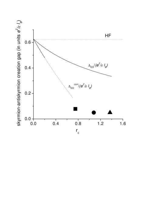
FIG. 1.: The normalized creation gap of the ED Hamiltonian model and the corrected gap are shown above. The dotted line represents the HF approximation result. The experimental data (closed symbols) are from Refs. 3 (the square), 4 (the circle), and 5 (the triangle).

Such results for $\Delta_{\mbox{ED}}$ and for $\Delta_{\mbox{ED}}^{\mbox{corr}}$ demonstrate a significant role of the LL mixing. The curves in Fig. 1 become closer to experimental data (c.f. the HF value shown by the dotted line). We demonstrate here only the data found at fairly strong magnetic fields, namely: $B=11.6,\;5.5\;\;\mbox{and}\;\;3.5\,$T correspondingly in Refs. [13, 16, 15]. Meanwhile, it should be noted, that the creation gap experimentally observed depends sharply on the effective $g$ factor in the vicinity of $g=0$ [in accordance with the low $(g\ln g)^{1/3}$, see Ref. [1]]. The result presented in the work of Ref. [13] and marked here by the square is really obtained at zero Zeeman energy (to an experimental accuracy). The measurements [15, 16] are carried out at small, but still not vanishing $g$ factors. Therefore, we have extrapolated these data to the point $g=0$. The results of this conventional extrapolation are presented in Fig. 1 by the closed triangle and the circle .

At the same time, the dashed line for value $\Delta_{\mbox{ED}}^{\mbox{corr}}$ evidently presents an underestimated result. In the higher order corrections in terms of $r_{\mbox{C}}$ the curve corresponding to the true energy gap should pass somewhere between the curves of Fig. 1 (the smaller the parameter $r_{\mbox{C}}$ is, the closer this true gap should be to the calculated value $\Delta_{\mbox{ED}}^{\mbox{corr}}$). In the ideal 2D case the results $\Delta_{\mbox{ED}}$ and $\Delta_{\mbox{ED}}^{\mbox{corr}}$ calculated for $r_{\mbox{C}}\sim 1$ may be considered as upper and lower limits for a real creation gap.

Finally we should emphasize that at least two important effects have been ignored with the calculation of the Fig. 1 curves: finite thickness (FT) correction, and disorder broadening of Landau levels (LL’s). Both of these reduce the energy gap. The usual way to take into account the FT is to modify the Coulomb interaction: $V(q)=2\pi F(q)/q$, where the formfactor $F$ is parameterized by an effective thickness.[41] Any second-order correction in terms of $r_{\mbox{C}}$ would involve this formfactor doubled and therefore, it would be more sensitive to the FT effect. Roughly speaking: a 30% reduction due to the FT correction to the spin-flip-mode energy (3.16) causes the corresponding correction to $\Delta_{\mbox{ED}}$ [see Eq. (3.20)] and determines a reduction by $\approx 50\%$ in $\Delta E^{(2)}$ [also by a factor of $\approx(0.7)^{\kappa}$ in the following $\Delta E^{(\kappa)}$ corrections]. The two curves $\Delta_{\mbox{ED}}$ and $\Delta_{\mbox{ED}}^{\mbox{corr}}$ would start thereby at $r_{\mbox{C}}=0$ from $\approx 0.7\sqrt{\pi/8}$ and become more sloping. At any $r_{\mbox{C}}$ the gap turns out to be smaller because of the FT effect.

The disorder may govern QHF features critically and even in the ground state this can lead to a realignment of spins with respect to one another. Specifically, the calculation of disorder effects depends on the model for the random potential. The white noise potential (arising e.g. due to chargeless point defects available in the 2D channel) is considered in Ref. [42]. A perceptible change of the charge gap seems to be related to appearance of a skyrmion-like structure in the ground state. The authors[42] found that the latter occurs at $\nu=1$ starting from some appreciable threshold for the amplitude of the disorder potential correlator. In the opposite case of long range potential fluctuations (mostly determined by charged impurities situated out of the spacer), the gap should change smoothly with correlator amplitude and could be estimated as follows. When chargeless exciton exists, the disorder broadening determines a finite cut-off value $q_{m}$ for 2D momenta: $q<q_{m}$. This momentum $q_{m}$ is related to a certain distance $l_{B}^{2}q_{m}$ (in usual units). At this distance a force of the Coulomb interaction between quasiparticles that form the exciton, becomes equal to an external random force appearing due to the disorder potential. Hence, the real creation gap for free quasiparticles decreases by a value $E_{x}(\infty)-E_{x}(q_{m})$, where $E_{x}(q)$ is an appropriate exciton energy calculated within the clean limit (c.f. the analysis in Refs. [23, 26]). It is rather difficult to estimate the gap reduction corresponding to our specific case, because the energy with $q$ of a skyrmion-antiskyrmion exciton is unknown. However, for the spin exciton[43, 44, 29] the analogous estimation [26] results in a reduction of $\approx 20\%$, if the random force is caused by distant impurities. (In real 2D structures this force could be estimated as $\sim 0.1\;$K/nm.)

Thus, the disorder and FT effects also play a role in the gap reduction at $r_{\mbox{C}}\sim 1$. However, for the up-to-date 2D structures they seem to be less important compared to the basic effect of the LL mixing.

 

ACKNOWLEDGMENTS

 

Useful discussions with A. M. Finkel’stein, S. V. Iordanskii, K. Kikoin, and Y. Levinson, are gratefully acknowledged. The author wishes to thanks for the hospitality the Department of Condensed Matter Physics of The Weizmann Institute of Science (Rehovot), where the significant part of this work was carried out. The work was supported by the MINERVA Foundation and by the Russian Fund for Basic Research.

 

APPENDIX I: MATRIX ELEMENTS

 

The commutation algebra (4.10a-d) for exciton operators (4.6) and (4.8) allows us with the help of the rule (4.9) to calculate the relevant matrix elements with relative ease. Using Eqs. (4.22), (4.4), (4.5), (4.23)-(4.25), (4.29), (4.30), and in view of the fact that ${\hat{Q}}_{\alpha\beta}^{+}\equiv{\hat{\cal Q}}_{\alpha\beta{\bf 0}}^{+}$ we find

$$\left\langle\alpha\left|{\hat{\cal H}}_{\mbox{{int}}}\right|0\right\rangle=\frac{e^{2}}{\varepsilon{}l_{B}}g_{\alpha}^{(a)}\,,$$

where

$$g_{\alpha}=\frac{V(q_{\alpha})(-1)^{n_{a_{1}}}\left({q_{\alpha}}_{-}\right)^{n_{a_{1}}+n_{a_{2}}}}{2\pi\sqrt{n_{a_{1}}!n_{a_{2}}!}}e^{-q_{\alpha}^{2}/2}\delta_{\sigma_{a_{1}},\frac{1}{2}}\delta_{\sigma_{a_{2}},\frac{1}{2}}\,;$$

and

$$\left\langle\alpha\left|\left[{\hat{\cal H}}_{\mbox{{int}}},{\hat{Q}}_{0\overline{1}}^{+}\right]\right|0\right\rangle=\frac{e^{2}}{\varepsilon{}l_{B}{N_{\phi}}^{1/2}}f_{\alpha}^{(a)}\,,$$

where

$$\begin{array}[]{lcl}\!\!f_{\alpha}=\frac{\displaystyle V(q_{\alpha})(-1)^{n_{a_{2}}}\left({q_{\alpha}}_{-}\right)^{n_{a_{1}}+n_{a_{2}}-1}}{\displaystyle 2\pi\sqrt{n_{a_{1}}!n_{a_{2}}!}}e^{-q_{\alpha}^{2}/2}{}{}\\ \vphantom{0000}\\ \!\!{\displaystyle\times}\left\{\begin{array}[]{ccr}0,&\mbox{if}&\sigma_{a_{1}}+\sigma_{a_{2}}\not=0,\\ L_{1}^{n_{a_{1}}-1}(q_{\alpha}^{2}/2),&\mbox{if}&\sigma_{a_{1}}=-\frac{1}{2},\>\>\sigma_{a_{2}}=\frac{1}{2},\\ -L_{1}^{n_{a_{2}}-1}(q_{\alpha}^{2}/2),&\mbox{if}&\sigma_{a_{1}}=\frac{1}{2},\>\>\sigma_{a_{2}}=-\frac{1}{2}.\\ \end{array}{}\;\;(\mbox{A}1.4)\right.\\ \end{array}$$

In the case of the state $|\beta\rangle$ corresponding to $\delta S_{z}=0$ (i.e. $\sigma_{b_{1}}=\sigma_{b_{2}}=1/2$) and in view of Eqs. (3.12), (4.24), (4.34) and (4.35) we obtain

$$\left\langle\alpha\left|\left[{\hat{\cal W}},{\hat{P}}_{\beta}^{+}\right]\right|0\right\rangle=d_{\alpha\beta}-\frac{1}{N_{\phi}}\sum_{\gamma}{\cal F}_{\alpha\gamma}d_{\gamma\beta}\equiv d_{\alpha\beta}^{(a)}\,,$$

where

$$d_{\alpha\beta}=\Omega^{+}_{-}\left(\sqrt{n_{b_{1}}+1}\delta_{\alpha,\beta_{1+}}+\sqrt{n_{b_{2}}+1}\delta_{\alpha,\beta_{2+}}\right)$$

$$+\Omega^{+}_{+}\left(\sqrt{n_{b_{1}}}\delta_{\alpha,\beta_{1-}}+\sqrt{n_{b_{2}}}\delta_{\alpha,\beta_{2-}}\right),$$

and indexes $\beta_{1\pm}$ and $\beta_{2\pm}$ designate the states

$$\!\!\left|\beta_{1\pm}\right\rangle=\left|\overline{n_{b_{1}}\pm 1},n_{b_{2}},{\bf q}_{\beta}\right\rangle,\;\,\left|\beta_{2\pm}\right\rangle=\left|n_{b_{1}},\overline{n_{b_{2}}\pm 1},{\bf q}_{\beta}\right\rangle.$$

[See definitions (4.35), (4.25), and (3.9).] In case $n_{a_{1}}\!\!+\!n_{a_{2}}=n_{b_{1}}\!\!+\!n_{b_{2}}$, we find also that for any function $v_{\alpha}$,

$$\sum_{\gamma}v_{\gamma}d^{*}_{\gamma\alpha}d_{\gamma\beta}=\delta_{\alpha,\beta}\left[\Omega^{+}_{-}\Omega^{-}_{+}v_{\beta_{1+}}\left(n_{b_{1}}+n_{b_{2}}+2\right)\right.$$

$$\left.+\Omega^{-}_{-}\Omega^{+}_{+}v_{\beta_{1-}}\left(n_{b_{1}}+n_{b_{2}}\right)\right].$$

Finally,

$$\left\langle\mbox{SF}\left|{\hat{\cal W}}\right|0\right\rangle=N_{\phi}^{1/2}\,.$$

 

APPENDIX II: THE COINCIDENCE

OF THE $r_{\mbox{C}}\!\to\!0$ RESULTS at $\nu=1$

 

We investigate the origin of the coincidence of our results, which are exact at $r_{\mbox{C}}\!\to\!0$, with the results obtained: (i) within the HF and WFP approximations;[5] (ii) within the HF approximation[7, 8]. In any case the gap has to be proportional to $e^{2}/\varepsilon l_{B}$. However, generally, the specific factor should be different in these three approaches.

In the work[5], where only a single LL is considered, the corresponding factor is determined by the $q^{2}$ term of the expansion of ${\cal E}_{\mbox{{sw}}}(q)\approx q^{2}{\cal E}_{\mbox{{sw}}}^{\prime\prime}(0)/2$ at a small wave vector $q$. Here ${\cal E}_{\mbox{{sw}}}(q)$ is the energy of spin exciton[29, 44]. [This value is equal to ${\cal E}_{0\overline{0}}(q)$ in our notations, see (3.9b) and (4.15)]. The creation gap in the work of Ref. [5] turns out to be equal to the inverse spin-exciton mass $M^{-1}_{\mbox{{sw}}}={\cal E}_{\mbox{{sw}}}^{\prime\prime}(0)$.

In the work of Ref. [7] both $n=0$ and $n=1$ LL’s are used for the presentation of the bare one-electron GF. In so doing, the external HF field for this GF has been taken into account. Therefore, the denominators of the GF contain the energies of one electron placed at the $n=1$ LL in its spin “up” and spin “down” states. The result for the skyrmion-creation gap turns out to be proportional to the difference of these $n=1$ energies. At the same time, the electron energies can be measured from the energy of a distant hole at the $n=0$ level. Then, the required difference corresponds to the extreme case (i.e. to the $q\!\to\!\infty$ limit) of the difference of the corresponding exciton energies:[29, 37] $E_{1}=\left.\left[{\cal E}_{0\overline{1}}(q)-{\cal E}_{01}(q)\right]\right|_{q\!\to\!\infty}$. [The energies ${\cal E}_{01}(q)$ and ${\cal E}_{0\overline{1}}(q)$ may be found directly from Eq. (4.15).]

We remind that our $r_{\mbox{C}}\!\to\!0$ result for the gap is ${\cal E}^{\mbox{{SF}}}_{01}\equiv{\cal E}_{0\overline{1}}(0)$. Thus, generally, these three different approaches should lead to the different results. However, due to specific features of the QHF studied, all these three values actually are equal to each other:

$$M^{-1}_{\mbox{{sw}}}=E_{1}={\cal E}^{\mbox{{SF}}}_{01}\equiv\frac{e^{2}}{\varepsilon l_{B}}\int\frac{d^{2}{\bf q}}{(2\pi)^{2}}\frac{q^{2}V(q)}{2}e^{-q^{2}/2}\,.$$

In particular, the coincidence of ${\cal E}^{\mbox{{SF}}}_{01}$ and $E_{1}$ is the result of the “accidental” equality of the $q=0$ and $q=\infty$ exchange energies for the 01-magnetoplasmon. Therefore, the Eqs. (A2.1) appear to be nothing more than an coincidence peculiar to the system studied.

If we study a single skyrmion or antiskyrmion, then we see that their energies (3.19) are determined also by an additional correction proportional to $q_{\mbox{T}}$ (where $q_{\mbox{T}}=\pm 1$). In fact, this correction in the present work as well as in Refs. [7, 8] is determined by the rotation-matrix feature (3.18) and by the renormalization rule (3.4). Therefore, under the coincidence condition (A2.1), we arrive again at the identical results. The approach of Ref. [5] seems indirectly to contain also certain features analogous to (3.4) and (3.18). Also it results thereby in the same energies of an isolated skyrmion or antiskyrmion.

Finally, it should be noted that for the filling $\nu\geq 3$ our result (3.25) differs from the result of Ref. [5]. This fact reflects the role of low lying LL’s which participate in the skyrmion formation. Nevertheless, the $\nu\geq 3$ skyrmion creation gap, just as in the approach adopted in Ref. [5], turns out to be lower than the corresponding quasiparticle gap. (In the work of Ref. [7] only the $\nu=1$ case was studied.)

REFERENCES

• [1] C. L. Sondhi, A. Karlhede, S. A. Kivelson, and E. H. Rezayi, Phys. Rev. B 47, 16419 (1993).
• [2] K. Moon, H. Mori, Kun Yang, S. M. Girvin, and A. H. MacDonald, Phys. Rev. B 51, 5138 (1995).
• [3] B. Králik, A. M. Rappe, and S. G. Louie, Phys. Rev. B 52, 11626 (1995).
• [4] H. A. Fertig, L. Brey, R. Côté, and A. H. MacDonald, Phys. Rev. B 50, 11018 (1994).
• [5] Yu. A. Bychkov, T. Maniv, and I. D. Vagner, Phys. Rev. B 53, 10148 (1996).
• [6] H. A. Fertig, L. Brey, R. Côté, and A. H. MacDonald, A. Karlhede, and S. L. Sondhi, Phys. Rev. B 55, 10671 (1997).
• [7] S. V. Iordanskii, S. G. Plyasunov, and V. I. Falko, Zh. Éksp. Teor. Fiz. 115, 716 (1999) [JETP 88, 392 (1999)].
• [8] S. V. Iordanskii and A. Kashuba, private communication.
• [9] S. E. Barret, G. Dabbagh, L. N. Pfeifer, K. W. West, and R. Tycko, Phys. Rev. Lett. 74, 5112 (1995).
• [10] I. Kukushkin, K. v. Klitzing, and K. Eberl, Phys. Rev. B 60, 2554 (1999).
• [11] V. Bayot, E. Grivei, S. Melinte, M. B. Santos, and M. Shayegan, Phys. Rev. Lett. 76, 4584 (1996)
• [12] A. Schmeller, J. P. Eisenstein, L. N. Pfeiffer, and K. W. West, Phys. Rev. Lett. 75, 4290 (1995).
• [13] D. K. Maude, M. Potemski, J. C. Portal, M. Heinini, L. Eaves, G. Hill, and M. A. Pate, Phys. Rev. Lett. 77, 4604 (1996).
• [14] D. R. Leadley, R. J. Nicholas, D. K. Maude, A. N. Utjuzh, J. C. Portal, J. J. Harris, and C. T. Foxon, Semicond. Sci. Technol. 13 671 (1998).
• [15] S. Melinte, E. Grivei, V. Bayot, and M. Shayegan, Phys. Rev. Lett. 82, 2764 (1999).
• [16] S. P. Shukla, M. Shayegan, S. R. Parihar, S. A. Lion, N. R. Cooper, and A. A. Kiselev, Phys. Rev. B 61, 4469 (2000).
• [17] A. A. Belavin and A. M. Polyakov, Pis’ma Zh. Éksp. Teor. Fiz. 22, 503 (1975) [JETP Lett. 22 245 (1975)].
• [18] R. Rajaraman, Solitons and Instantons (North-Holland, Amsterdam, 1989).
• [19] A. B. Dzyubenko and Yu. E. Lozovik, Fiz. Tverd. Tela (Leningrad) 25, 1519 (1983) [Sov. Phys. Solid State 25, 874 (1983)]; Fiz. Tverd. Tela (Leningrad) 26, 1540 (1983) [Sov. Phys. Solid State 26, 938 (1984)].
• [20] A. B. Dzyubenko and Yu. E. Lozovik, J. Phys. A 24, 415 (1991).
• [21] Yu. A. Bychkov and S. V. Iordanskii, Fiz. Tverd. Tela (Leningrad) 29, 2442 (1987) [Sov. Phys. Solid State 29, 1405 (1987)].
• [22] S. Dikman and S. V. Iordanskii, Zh. Éksp. Teor. Fiz. 110, 238 (1996) [JETP 83, 128 (1996)].
• [23] S. Dickmann and Y. Levinson, Phys. Rev. B 60 7760 (1999).
• [24] S. Dikman and S. V. Iordanskii, Pis’ma v Zh. Eksp. Teor. Fiz. 70, 531 (1999) [JETP Lett. 70, 543 (1999)].
• [25] S. Dickmann and Y. Levinson, Physica E 5, 153 (1999).
• [26] S. Dickmann, Phys. Rev. B 61, 5461 (2000).
• [27] L. D. Landau and E. M. Lifschitz, Quantum Mechanics (Butterworth-Heinemann, Oxford, 1991).
• [28] The gradient expansion is the expansion in terms of the small parameter ${}l_{B}/R$, in which $R$ is a skyrmion radius. The latter is determined by the ratio of the Zeeman energy to the Coulomb energy $e^{2}/\varepsilon{}l_{B}$. In our study, the Zeeman energy does not appear. We obtain the results of the skyrmion energy to the zero order of ${}l_{B}/R$.
• [29] C. Kallin and B. I. Halperin, Phys. Rev. B 30, 5655 (1984).
• [30] According to Larmor’s theorem there are also pure spin excitations (having the Zeeman gap) which do not change the space wave function of the ground state, and therefore they do not influence the activation gap.
• [31] W. Kohn, Phys. Rev., 123, 1242 (1961).
• [32] B. Huckestein and M. Backhaus, cond-mat/0004174 (2000), to appear in Advances in Solid State Physics Vol. 42, B. Kramer (ed.), Springer-Verlag, Heidelberg (2002).
• [33] S. Chakravarty, S. Kivelson, C. Nayak, and K. Voelker, Phil. Mag. B 79, 859 (1999).
• [34] I. Mihalek and H. A. Fertig, Phys. Rev. B 62, 13573 (2000).
• [35] For the third Eulerian angle $\zeta$ we have set $\zeta=\varphi$ in accordance with Ref. [7]. Final results do not depend on $\zeta$, but this substitution enables us to avoid some non-physical singularities of intermediate results.
• [36] It is noted that the state $|0\rangle$ is degenerate, since any state $\left(\sigma_{-}\right)^{m}|0\rangle$ has the same energy to the zero order of ${\hat{V}}_{\Omega}$. In the first and second approximations, in terms of ${\hat{V}}_{\Omega}$, we arrive at a quantum tunneling from $|0\rangle$ to $\sigma_{-}|0\rangle$. However, this results only in the correction of the order of $\omega_{c}\sqrt{N_{\phi}}{}l_{B}^{2}\nabla^{2}$ to the energy that is by the factor $\sim 1/\sqrt{N_{\phi}}$ smaller than the studied result relevant for the $G_{i}$ region.
• [37] J. P. Longo and C. Kallin, Phys. Rev. B 47, 4429 (1993).
• [38] A. Pinczuk, B. S. Dennis, D. Heiman, C. Kallin, L. Brey, C. Tejedor, S. Schmitt-Rink, L. N. Pfeiffer, and K. W. West, Phys. Rev. Lett. 68, 3623 (1992).
• [39] Yu. A. Bychkov, and E. I. Rashba, Zh. Eksp. Teor. Fiz. 85, 1826 (1983) [Sov. Phys. JETP 58, 1062 (1983)].
• [40] We can compare these results with the $r_{\mbox{C}}^{2}$ corrections to the energies of the simple $S_{z}=-1/2$ excitations (quasielectrons and quasiholes). In this case the studied states are $b^{+}_{p}|0\rangle$ and $a_{p}|0\rangle$, where the sublevel indexes are $a=(0,+1/2)$ and $b=(0,-1/2)$. The results of the second-order perturbation theory are obtained with the use of the operator (4.20). The energy corrections measured from the ground state (which must be calculated also to the same order) can be found analytically by carrying out the corresponding summations: $E^{(2)}_{e}=-\frac{\pi^{2}}{24}-\frac{1}{4}(\ln{2})^{2}=-0.531...$ and $E^{(2)}_{h}=-\frac{\pi^{2}}{24}+\frac{3}{4}(\ln{2})^{2}=-0.0509...$ (in units of $2\,$Ry$=r_{\mbox{C}}^{2}\omega_{c}$). These values differ slightly from the numerical results presented in Ref. 1.
• [41] T. Ando, A. B. Fowler, and F. Stern, Rev. Mod. Phys. 54, 437 (1982).
• [42] J. Sinova, A. H. MacDonald, and S. M. Girvin, Phys. Rev. B 62, 13579 (2000).
• [43] I. V. Lerner and Yu. E. Lozovik, Zh. Eksp. Teor. Fiz. 78, 1167 (1980) [Sov. Phys. JETP 51, 588 (1980)].
• [44] Yu. A. Bychkov, S. V. Iordanskii, and G. M. Éliashberg, Pis’ma Zh. Eksp. Teor. Fiz. 33, 152 (1981) [Sov. Phys. JETP Lett. 33, 143 (1981)].