Probability distribution of the sizes of largest erased-loops in loop-erased random walks

Abstract

We have studied the probability distribution of the perimeter and the area of the $k$th largest erased-loop in loop-erased random walks in two-dimensions for $k$ = $1$ to $3$. For a random walk of $N$ steps, for large $N$, the average value of the $k$th largest perimeter and area scales as $N^{5/8}$ and $N$ respectively. The behavior of the scaled distribution functions is determined for very large and very small arguments. We have used exact enumeration for $N\leq 20$ to determine the probability that no loop of size greater than $\ell$ is erased. We show that correlations between loops have to be taken into account to describe the average size of the $k$th largest erased-loops. We propose a one-dimensional Levy walk model which takes care of these correlations. The simulations of this simpler model compare very well with the simulations of the original problem.

]

I INTRODUCTION

The classical theory of statistics of extremals deals with the distribution of the largest of many independent identically distributed random variables [3, 4]. After some rescaling, this distribution tends to one of the three universal distribution functions, the so-called Gumbel distributions, independent of the details of the starting distribution of random variables [5]. The independence of random variables is, however, not a good approximation in many physical problems. The statistics of extremes of many random variables is relevant in many different physical contexts. In many of these it is important to take account of correlations, for example, in the study of earthquakes [6], weather records [7], slow relaxation in glassy systems [8], and persistence in random walks [9]. In some special cases extremal statistics of strongly correlated variables can be determined exactly [10]. In general, however, the study of extremal distributions of correlated and strongly correlated random variables poses a rather non-trivial problem even in the simplest cases.

This paper deals with the extremal statistics of variables with long-range power law correlations in the loop-erased random walks (LERW’s) in two dimensions. Our interest in the LERW problem comes from the fact that it provides one of the simplest examples of self-organized critical systems. In the LERW problem, the length of the walk is first increased by one at each step, and then decreases by a random amount due to possible loop erasures. The size of erased loops has a power-law tail [11]. This is, thus, similar to the sandpile model where one grain is added at each time step but the number of grains leaving the pile has a power-law tail. Clearly, there are correlations in the sizes of erased loops at different times. These correlations are more pronounced for larger loops. Erasure of a large loop leads to significant decrease in the length of the erased walk, and hence a significant decrease in the probability of erasure of another large loop within a short time. We propose that the expected ratios of sizes of $k$th largest loop with the largest loop is a good variable to quantify these strong correlations, and propose a one-dimensional Levy walk model which is then tested by simulations.

The LERW problem was introduced by Lawler [12] as a more tractable variant of the self-avoiding walk problem. This problem is related to many well-studied problems in statistical physics: the classical graph-theoretical problem of spanning trees, the $q$-state Potts model in the limit $q\to 0$ [14], and the Laplacian self-avoiding walk problem [13]. Connection to the spanning trees also relates this problem to the abelian sandpile model of self-organized criticality [15]. Recently simulation of LERW has been used as a computationally efficient way to determine the dynamical exponent of the abelian sandpile model in three-dimensions [16]. The upper critical dimension of LERWs is known to be 4 [17]. In two dimensions, the fractal dimension of LERWs is known to be $5/4$ [14, 18, 19], and the exponent characterizing the probability distribution of the area of erased-loops is known to be superuniversal [16]. Several other results on LERWs can be found in [11, 20, 21, 22] and a good review of earlier results on the LERW problem can be found in [17].

In this paper, we show that the asymptotic behavior of the probability distribution function $\text{Prob}(\ell^{(k)}|N)$ that the $k$th largest erased-loop perimeter in the first $N$ steps has value $\ell^{(k)}$ is described by a $k$-dependent scaling function with argument $\ell^{(k)}/N^{z/2}$. We determine the behavior of the scaling function for the largest loop for very large and very small values of its argument. A similar behavior is found for the loops ranked by the enclosed area, rather than by their perimeter. The probability that there is no erased loop of length greater than a fixed value $r$ varies exponentially with $N$ for large $N$. Enumerating all walks satisfying this property (for a fixed $r$) is a generalization of the self-avoiding walk problem. We have used exact enumeration techniques to determine the behavior of this probability for $r=0$, $2$, and $4$ by enumerating all random walks with $N\leq 20$. We have proposed a simple Levy walk model which captures correlations in the LERW and agrees well with its extremal statistics as determined from large-scale Monte Carlo simulations.

The plan of this paper is as follows: In Sec. II, after defining the LERW model precisely, we recall relevant points from scaling theory for distribution of sizes of erased-loops. These are used to get the scaling form for the probability distribution of the perimeter and the area of largest erased-loop in a walk of $N$ steps. In Sec. III, we outline our results about the connectivity constants $\mu_{2}$ and $\mu_{4}$ and determine their numerical value using series expansions. The simulation technique and results obtained thereof are described in Sec. IV. In Sec. V, we describe the Levy walk model and compare the results of numerical simulations of this model with that of the LERW. Finally, some concluding remarks follow in Sec. VI.

II Scaling Theory of loop-size Distributions

A loop-erased random walk is defined recursively as follows: For a one step random walk, the corresponding loop-erased random walk is the same as the random walk. To form the LERW ${\cal L}^{\prime}$ corresponding to a given random walk of $(N+1)$ steps, we first form the LERW ${\cal L}$ corresponding to the first $N$ steps of the random walk. Let us say this LERW ${\cal L}$ has $n$ steps. We now add the $(N+1)$th step of the random walk to ${\cal L}$. If no loop is formed, the resulting $n+1$ stepped walk is ${\cal L}^{\prime}$. If this results in forming a loop of perimeter $\ell$, this loop is erased, and the resulting $n+1-\ell$ stepped walk is ${\cal L}^{\prime}$. A simple example is depicted in Fig. 1.

Let ${\cal L}$ be a LERW of $n$ steps obtained from a random walk of $N$ steps. For a fixed $N$, $n$ is a random variable. The critical exponent $z$ of the LERW is defined by the relation that

$$\langle n\rangle\sim N^{z/2}$$ (1)

for large $N$, where the angular brackets denote ensemble averaging over all random walks of $N$ steps. Since the root-mean-square end to end distance $R$ for LERWs is the same as that for random walks, we have $R\sim N^{1/2}$, and $\langle n\rangle\sim R^{z}$. Thus, $z$ is the fractal dimension of the LERW.

Let $F(\ell|N)$ be the cumulative probability that a loop of perimeter greater than $\ell$ will be erased at the $N$th step of the loop-erased walk. We define

$$F(\ell)=\lim_{N\to\infty}F(\ell|N).$$ (2)

It was shown in [16] that large $N\gg\ell\gg 1$, $F(\ell|N)$ satisfies the scaling form

$$F(\ell|N)\sim\ell^{-2/z}f\bigl{(}\ell/N^{z/2}\bigr{)}.$$ (3)

The scaling function $f(x)$ tends to a non-zero constant as $x$ tends to zero, and decreases to zero exponentially fast for $x\gg 1$. Note that the exponents appearing in this scaling form depend only on the fractal dimension $z$.

Let $\Phi(\ell^{(1)}\leq\ell|N)$ be the cumulative probability that the perimeter $\ell^{(1)}$ of the largest erased-loop in an $N$-step walk will be less than or equal to $\ell$. We shall study the behavior of this function for large $N$. The probability that the largest erased-loop at the $k$th step of an $N$-step walk has perimeter less than or equal to $\ell$ is given by $1-F(\ell|k)$. A simple approximate formula for $\Phi(\ell^{(1)}\leq\ell|N)$ is obtained by neglecting correlations among sizes of erased-loops, and treating the generation of loops at different time steps as independent events. In the following, we will denote by $\Phi_{\text{uc}}$ the value of $\Phi(\ell^{(1)}\leq\ell|N)$ in this uncorrelated approximation. This gives

$$\Phi(\ell^{(1)}\leq\ell|N)\simeq\Phi_{\text{uc}}(\ell^{(1)}\leq\ell|N)=\prod_{k=1}^{N}[1-F(\ell|k)].$$ (4)

Let $x=\ell/N^{z/2}$, $x^{(1)}=\ell^{(1)}/N^{z/2}$ and $y=k/N$ be new scaling variables. In terms of these new variables, substitution of $F(\ell|k)$ from Eq. (3) in Eq. (4), gives

$$\Phi_{\text{uc}}(x^{(1)}\leq x|N)=\prod_{y}\left[1-\frac{1}{N}x^{-2/z}f\left(\frac{x}{y^{z/2}}\right)\right].$$ (5)

For fixed $x$ and large, we can evaluate this expression by taking logs, expanding in powers of $(1/N)$, and keeping only the lowest order terms in $(1/N)$. With this we get

$$\ln\Phi_{\text{uc}}(x^{(1)}\leq x|N)=-x^{-2/z}\tilde{f}(x),$$ (6)

where $\tilde{f}(x)=\int_{0}^{1}f\left(x/y^{z/2}\right)dy$. It is easy to see that $\tilde{f}(x)$ has the same qualitative behavior as $f(x)$. In terms of $F(\ell|k)$, this equation can be written as

$$\Phi_{\text{uc}}(\ell^{(1)}\leq\ell|N)\simeq\exp\left[-N\tilde{F}(\ell|N)\right],$$ (7)

where

$$\tilde{F}(\ell|N)=\frac{1}{N}\sum_{k=0}^{N}F(\ell|k).$$ (8)

For small $x$, $\ln\Phi_{\text{uc}}(x^{(1)}\leq x|N)$ should vary as $-x^{-2/z}$. For large $x$, $\tilde{f}(x)$ is small, and $1-\Phi_{\text{uc}}(x^{(1)}\leq x|N)$ should vary as $x^{-2/z}\tilde{f}(x)$.

Eq. (7) is a good approximation to Eq. (4) so long as the higher order terms in $(1/N)$ can be neglected. It is easily seen that the neglected term is of order $N\tilde{F}^{2}(\ell|N)$, and hence the approximation is valid so long as $\ell\gg N^{z/4}$. It will be seen from simulation results (see Sec. IV) that our assumption about correlations being small is not too bad and that Eq. (4), and consequently also Eqs. (6) and (7), are reasonable approximations to the largest loop size distribution for all $\ell$. The deviation of the correct value from Eq. (4) is largest if $\ell$ is very small, say equal to $0$, $2$, $4$, …. It is important to understand the behavior of $\Phi(\ell^{(1)}\leq\ell|N)$ in this case. This we do in the next section.

Let $m$ be the expected number of loops of perimeter greater than or equal to $\ell$ generated from a random walk of $N$ steps. If there are no correlations between different loops, for $m\ll N$, the number of such loops generated in particular realization is a random variable, distributed according to the Poisson distribution: The probability that exactly $k$ such loops are generated is $\text{e}^{-m}m^{k}/k!$. This implies that the probability that less than $k$ loops of size greater than $\ell$ are generated can be expressed in terms of the probability that no loop of size greater than $\ell$ is generated. Simple algebra gives

$$\Phi_{\text{uc}}(\ell^{(k)}\leq\ell,N)=\exp(-m)\sum_{i=0}^{k-1}\frac{m^{i}}{i!},$$ (9)

where

$$m=-\log(\Phi_{\text{uc}}(\ell^{(1)}\leq\ell|N)).$$ (10)

III DETERMINATION OF CONNECTIVITY CONSTANTS

Let $C_{r}(N)$ be the number of $N$-step random walks in which no loop of size greater than $r$ is formed. The case $r=0$ corresponds to self-avoiding walks. As the total number of random walks of $N$-steps is $4^{N}$ on square lattice, we have

$$\Phi(\ell^{(1)}\leq r|N)=\frac{C_{r}(N)}{4^{N}}.$$ (11)

For large $N$ it is expected that [24]

$$C_{r}(N)\sim\mu_{r}^{N}.$$ (12)

For large $N$, $\mu_{r}$ tends to a constant independent of $N$, which may be called the “$r$-th connectivity constant”. From Jensen and Guttmann [23] the value of $\mu_{0}$ is known very precisely and we have estimated $\mu_{2}$ and $\mu_{4}$ using series expansion and exact enumeration (details follow).

Now consider the case $k=2$. In this case, the walk cannot form loops, except that it can go back along the path it has taken. The connectivity constant $\mu_{0}$ can be interpreted as the average number of forward directions available for the next step in an $N$-step self-avoiding walk for large $N$. As return along the direction of last step is now allowed, in the first approximation, we should have

$$\mu_{2}\approx\mu_{0}+1$$ (13)

We also have the trivial inequality $\mu_{r}<\mu_{r+2}$ for all $r$. As $r$ tends to infinity, $\mu_{r}$ tends to $4$.

We determined the numbers $C_{r}(N)$ for $N\leq 20$ and for all $r$ by exact enumeration. The enumeration results for $r=2$ and $4$ are tabulated in Table I. We analyzed this data by fitting it to the extrapolation form

$$C_{r}(N) = K_{0}\mu_{r}^{N}(N)N^{\gamma-1}$$ (15)

$$\times\left[1+\frac{K_{1}}{N}+\frac{(-1)^{N}}{N^{\gamma+1/2}}\left\{K_{2}+\frac{K_{3}}{N}\right\}\right],$$

where the critical exponent $\gamma$ is expected to be independent of $r$ and takes the self-avoiding walk value of $43/32$ in two dimensions [24] and $K_{i}$ are constants which depend on $r$. This form is similar to that used by Conway and Guttmann [24] for analyzing $51$-term series of self-avoiding walks. We have reduced the number of parameters in Eq. (15) because our series is shorter. Our estimates of $\mu_{2}$ and $\mu_{4}$, by fitting the form given by Eq. (15) term-by-term to the $20$-term series tabulated in Table I, are $3.7083(2)$ and $3.8818(4)$, respectively. These values are not very sensitive to variation in the fitting values of the parameters $K_{i}$.

It is interesting to compare the numerical values of $\mu_{0}$, $\mu_{2}$, and $\mu_{4}$ with the estimates obtained using the uncorrelated approximation. From Eqs. (11) and (12) we see that $\Phi(\ell^{(1)}\leq\ell|N)$ varies as $(\mu_{\ell}/4)^{N}$ for large $N$. Thus the approximation Eq. (7) gives $\mu_{k}/4\approx 1-F(k)$. Using the values of $\mu_{k}$ determined above, this would imply that $F(0)$, $F(2)$, and $F(4)$ have the values $0.3404$, $0.0729$, and $0.0295$, respectively. The values of these quantities obtained from simulations are $0.3125$, $0.0625$, and $0.0257$, respectively. We see that the approximation fares rather well in relating the properties of the self-avoiding and loop-erased walks, which have quite different large-scale properties.

IV COMPUTER SIMULATION RESULTS

We generated two-dimensional loop-erased random walks using the algorithm outlined in [16]. For each walk we collected statistics about the perimeter and the area of the erased-loop at each step. The statistics were collected for $N$-step walks with $N=2^{r}$, $r=15$, $\cdots$, $20$. We averaged over $4.7\times 10^{5}$ different realizations of the random walk. We were able to simulate the entire ensemble in about $93$ hours on a Pentium-III 700 MHz machine using about $2.6$ Mb RAM.

A Largest loop perimeter

During the simulations we collected statistics for $\tilde{F}(\ell|N)$, the average number of loops of perimeter $\ell$ formed from a random walk of $N$ steps. For each walk we also determined the perimeter and area of the five largest loops formed. this is used to obtain the measured cumulative distribution $\Phi_{\text{o}}(\ell^{(k)}\leq\ell|N)$, of size of loops of rank $k$, with $k=1$ to $5$. The subscript “o” here refers to “observed”. To reduce noise, nearby $\ell$ values were binned together. We used $30$ bins per decade of data.

In Fig. 2 we have shown the plot for $\text{Prob}_{\text{o}}(\ell^{(k)}|N)$ versus $\ell$ the observed probability distributions for $k=1$, $2$, and $3$ for $N=2^{20}$. In Fig. 3 we have plotted $\Phi(\ell^{(k)}\leq\ell|N)$ versus $\ell/\ell^{\star}$ for various values of $N$ as found in the simulations, and compared it to the theoretical curve given by Eq. (9) ignoring correlations between loops. An excellent collapse is seen among curves for all the values of $N$ when plotted against the scaling variable $x=\ell/\ell^{\star}$. From these figures it is clearly seen that for $x>1$ the prediction of the uncorrelated theory is quite good and indeed asymptotically exact. However, considerable departure is seen for smaller values of $x$, for $x\ll 1$.

We see that the prediction of the cumulative distribution function by the uncorrelated theory is consistently higher compared to the observed distribution throughout the range of variation of the scaling variable $x$. This shows the expected anti-correlation between occurrences of large loops.

For small values of the scaling parameter $x$, the observed cumulative distribution function seems to behave like

$$\Phi_{\text{o}}(x^{(1)}\leq x)\sim a\exp(-bx^{-2/z})$$ (16)

with $a=2.2\pm 0.3$ and $b=0.39\pm 0.02$. The fit is shown in Fig. 4. For large $x$, $1-\Phi_{\text{o}}(x^{(1)}\leq x)$ is very nearly $N\tilde{F}(\ell|N)$ which varies as

$$1-\Phi_{\text{o}}(x^{(1)}\leq x)\sim a\exp(-bx^{2/z})$$ (17)

with the numerical value of the parameters obtained by curve-fitting being $a=0.32\pm 0.03$ and $b=1.7\pm 0.1$, same as that obtained by analysis of the all-loops data. This fit is shown in Fig. 5.

B Largest loop area

During simulations we collected statistics for the area of the erased-loops also. This was sampled exactly as the perimeter data in the previous subsection.

In Figs. 6 and 7 we have shown the plots for $\text{Prob}_{\text{o}}(A^{(k)}|N)$ versus $A$ for $N=2^{20}$ and $\Phi(A^{(k)}\leq A|N)$ versus $A/N$ for various values of $N$, for $k=1$ to $3$. The format of presentation is as in the previous subsection. An excellent collapse is seen among the curves for various values of $N$ when plotted against the scaling variable $y=A/N$.

The departure between the observed behavior and prediction of the uncorrelated theory is also similar to that seen for the perimeter data in the previous subsection. It is clearly seen from these figures that for $y>0.1$ the prediction of the uncorrelated theory is quite good and seems to be asymptotically exact for large $y$. For $y<0.1$ considerable departure is seen between observed behavior and uncorrelated prediction. As in the perimeter data, there is a systematic over-prediction by the uncorrelated theory.

For small values of the scaling parameter $y$, the observed cumulative distribution function $\Phi_{\text{o}}(y^{(1)}\leq y)$ seems to behave like $\exp(-a/y)$ with $a=0.049\pm 0.002$. For large $y$, $1-\Phi_{\text{o}}(y^{(1)}\leq y)$ varies as $\exp(-by)$ with $b=14\pm 1$.

C Variation of loop sizes with rank

It is clearly seen in Fig. 2 that the probability distribution of $\ell^{(k)}$ becomes sharper as $k$ increases. In fact, if $k$ is of order $N$ (say $k=N/1000$), it is easy to see that the distribution tends to a delta function for large $N$. A more careful argument shows that if $k\gg N^{z/(z+1)}$, then the distribution would tend to a delta function. We note that $\ell^{(k)}$ varies as $(N/k)^{z/2}$ and the average number of erased loops with this perimeter varies as $N/(\ell^{(k)})^{1+2/z}$. For the distribution to have sharp peak at $\ell^{(k)}$, this number should be much greater than fluctuations in the expected number of loops with perimeter greater than $\ell^{(k)}$. The latter varies as $k^{1/2}$. Simple algebra then gives the required result.

A similar argument for the area distributions shows that the positions of the peak for the $k$-th rank varies roughly as $N/k$ and their width varies as $N/k^{3/2}$. Furthermore, when $k\gg N^{2/3}$ the width of the distribution becomes exponentially small in $N$.

D Affect of correlations on the probability distribution functions for $k$th largest erased-loop size

In Fig. 8, we have plotted $\Phi(\ell^{(2)}\leq\ell|N)$ and $\Phi(\ell^{(3)}\leq\ell|N)$ versus $\Phi(\ell^{(1)}\leq\ell|N)$ for $N=2^{20}$ from the observed distributions. This is compared with what would be expected on the basis of uncorrelated approximation. Similar plots using area (instead of perimeter) data show similar trends, and are omitted here. From this figure, it is clearly seen that the predicted and the observed distributions are quite close. The actual curve always lies above the value calculated by neglecting anti-correlations present.

V MODELING CORRELATIONS

Consider the time series $\{n_{i}\}$ with $i=1$, $2$, …, generated in a LERW simulation, where $n_{i}$ is number of steps in the LERW at time step $i$. This process can be modeled by a stochastic motion of point on a one dimensional lattice. As $n_{i}$ is always positive, the motion occurs in the half space $x\geq 0$. In a single time step, this point can move one step to the right (if no loop erasure occurs in the corresponding random walk), or several spaces to the left. Now suppose that the random walk is not accessible to observation, and only the time series $\{n_{i}\}$ is observed. While the original LERW, treated as a stochastic process is a Markov process, the projected process is clearly not Markovian. However, it may be approximated as a Markov process.

A One-dimensional Levy walk model

The transition probabilities for this Markov process are easily defined. We think of $n_{i}$ as the position of a random walker at time $i$ on a one dimensional lattice. The walk begins at $t=0$ with the walker positioned at $x=0$. At each subsequent time step, the walker takes one step to the right and then draws a non-negative integer random number $\ell$ with the probability $\text{Prob}(\ell)$, $\ell=0$, $1$, $2$, …. We will assume that for large $\ell$, $\text{Prob}(\ell)$ decreases as $\ell^{-\tau}$ with $\tau>1$. If $\ell$ is less than or equal to the current position $x$ of the walker, then the walker takes $\ell$ steps to the left; otherwise it stays put. This completes one step. Clearly, we have

$$\sum_{\ell=0}^{\infty}\text{Prob}(\ell)=1.$$ (18)

To ensure that there is no overall drift in the model, we also assume that

$$\sum_{\ell=0}^{\infty}\ell\text{Prob}(\ell)=1.$$ (19)

Note that the $\ell$ here corresponds to the erased-loop size in LERWs. In general, one can expect to improve comparison with the original LERW model by making the probability of backward $\ell$ steps when the walker is at $n$ equal to the conditional probability in the LERW problem that the next step leads to erasure of a loop of length $\ell$ when the current length of walk is $n$. This is expected to be of the form

$$\text{Prob}(\ell|n)=\text{Prob}(\ell|\infty)f_{\text{cutoff}}(\ell/n),$$ (20)

where $f_{\text{cutoff}}$ is a cutoff function which is strictly zero if its argument is greater than $1$. We make the simple choice that $f_{\text{cutoff}}$ is $1$ if the argument is less than $1$.

For our simulations, we made a particular choice of $\text{Prob}(\ell)$. We assumed that it is given by

$$\text{Prob}(\ell)=\left\{\begin{array}[]{ll}\displaystyle\frac{1}{\ell}\left[\frac{1}{\ell^{\alpha}}-\frac{1}{(\ell+1)^{\alpha}}\right],&\quad\text{for~{}}1\leq\ell\leq\infty\\ \\ \displaystyle 1-\sum_{k=1}^{\infty}\text{Prob}(k),&\quad\text{for~{}}\ell=0.\end{array}\right.$$ (21)

Note that with this choice, the no-drift condition given by Eq. (19) is automatically guaranteed for any choice of $\alpha$. Furthermore, one can generate this distribution numerically by using only two calls to the random number generator. We take a random number $u$ with uniform distribution between $[0,1]$, define $m=\lfloor u^{-1/\alpha}\rfloor$, and then put $\ell=m$ with probability $1/m$ and $\ell=0$ with probability $1-1/m$. In our simulations, we used $\alpha=0.6$, which corresponds to the value $\tau=2.6$ of the exponent of the two-dimensional LERWs.

The Master equation for the above process describing the evolution of the probability $P(x,t)$ of the walker being at position $x$ at time $t$ is written as

$$P(x,t+1)=\sum_{\ell=0}^{\infty}\text{Prob}(\ell)P(x-1+\ell,t).$$ (22)

For large times $t$, the width of the probability distribution $P(x,t)$ increases to infinity. It is easy to see that the width must increase as $t^{1/(1+\alpha)}$. We note that if the particle it at $x$, its expected displacement in the next time-step is positive, as jumps with displacement greater than $x$ to the left are disallowed. The contribution of such terms to Eq. (18) varies as $x^{2-\tau}$. This equation may schematically be written in the form

$$\frac{\partial P}{\partial t}\sim\frac{\partial}{\partial x}(Px^{2-\tau})+{\cal D}P,$$ (23)

where ${\cal D}$ denotes diffusion operator which, presumably, involves fractional derivatives. The resulting equation for the scaling function is nonlocal, and its analytical solution seems difficult. Simple dimensional analysis shows that $t$ scales as $x^{\tau-1}$. Hence the width of this distribution should scale as $t^{1/(\tau-1)}$. Furthermore, for large $t$, $P(x,t)$ tends to the scaling form

$$P(x,t)\simeq\frac{1}{t^{1/(\tau-1)}}p\left(\frac{x}{t^{1/(\tau-1)}}\right).$$ (24)

B Results from the Levy walk model

We numerically integrated the Master equation Eq. (22) in $x\geq 0$ half space using the probability distribution for erased-loop sizes given by Eq. (21) and computed $P(x,t)$. The integration for walks having up to $N=2^{17}$ steps required about $80$ hours of CPU time on a Pentium II 350 MHz machine using about $7$ Mb RAM. We also simulated the Levy walk process for time steps up to $N=2^{20}$ for obtaining the statistics on erased-loop sizes and the $k$th largest erased-loop size. The quantities were sampled along the same lines as for the LERWs discussed in Sec. IV. To reduce noise in the statistics, we averaged over a large ensemble consisting of $2\times 10^{5}$ different runs. The simulation of the entire ensemble required about $141$ hrs of CPU time on a Pentium II 350 MHz machine using about $1.5$ Mb RAM.

Scaling plots for the computed probability of finding the Levy walker at location $x$ at time step $N$, $P(x,N)$, are shown in Fig. 9. In this figures we have plotted $N^{z/2}P(x,N)$ versus $x/N^{z/2}$, for $z=5/4$. The figure clearly shows that the observed behavior agrees well with the conjectured scaling form given by Eq. (24).

We also analyzed the distribution of $k$th largest loop sizes in simulation of this Levy walk model, and compared them with the corresponding distributions for the two-dimensional LERW model. We found that the deviations from the predictions of the uncorrelated theory are much smaller in the case of the Levy walk model than in the original LERW. The plots are very similar to the Figs. 2, 3, and 8, and are being omitted here.

In Fig. 10, we have compared the probability distributions for the $k$th largest erased-loop sizes from the Levy walk model with those from LERW. The figure clearly shows that the probability distributions obtained from the Levy walk model match very well with those from the LERW.

A better quantitative estimate can be obtained by comparing the ratio $R_{k}$, defined as

$$R_{k}=\langle\ell^{(k)}\rangle/\langle\ell^{(1)}\rangle,$$ (25)

where $\langle\rangle$ denotes expectation value.

The value of $R_{k}$ as found in the simulations of the LERW was found to be $0.605$, $0.463$, $0.386$, and $0.335$ for $k=2$ to $5$, respectively. The corresponding values in the simulation of the Levy walk model were $0.614$, $0.474$, $0.397$, and $0.347$, respectively. The corresponding values from the uncorrelated approximation would be ${k}^{-z/2}$, i.e., $0.648,0.503,0.420$, and $0.365$, respectively. It is clear that the Levy walk model gives a much better estimate of these ratios than the uncorrelated approximation.

VI CONCLUDING REMARKS

Our analysis above shows that the probability distribution of the largest erased-loops in LERWs is fairly well described by the simple approximation ignoring correlations between the sizes of different loops. However, the average values of ratios of $\ell^{(k)}$ are not well described in this approximation. A simple model which takes care of a large part of these correlations is the Levy walk model introduced in this paper. In this model, one keeps information about the length of the LERW, but throws out all information about its shape. We have seen that this model reproduces the extremal statistics of the LERWs quite well.

Secondly, we have exactly enumerated $C_{r}(N)$ the number of $N$ step LERWs in which loops of size less than or equal to $r$ are erased. Using these we have determined $\mu_{r}$ the $r$th connectivity constant. The determination of $\mu_{0}$ for various lattices has been a long-standing problem in lattice statistics. Higher $r$-values present interesting geometrical questions, and may be helpful in understanding the crossover from random walk to self-avoiding walk.

TABLE I.: Number of $N$-step loop-erased random walks $C_{\ell}(N)$ in which the largest loop of perimeter $\ell$ less than or equal to $2$ and $4$ are erased for $N=1$, $\cdots$, $20$.

$N$	$C_{2}(N)$	$C_{4}(N)$
1	4	4
2	16	16
3	64	64
4	248	256
5	976	1024
6	3736	4072
7	14536	16248
8	55280	64352
9	213336	256120
10	808016	1011504
11	3099456	4016496
12	11706568	15828968
13	44696992	62727520
14	168475176	246805224
15	640913784	976340664
16	2411998168	3836482296
17	9148925856	15153764480
18	34387933200	59482843856
19	130125970320	234640138528
20	488603502672	920216177360

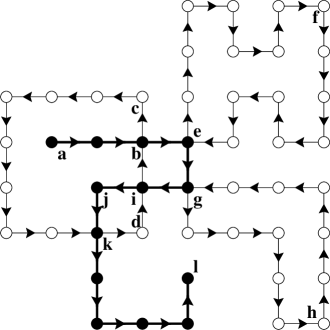
FIG. 1.: An illustrative example of the loop-erasure procedure and some aspects related to perimeter and enclosed area of erased-loops in loop-erased random walks: The random walk a-b-c-d-i-b-e-f-e-g-h-g-i-j-k-l of 52 steps starts at a, and ends at l. The erased-loops are shown by thin lines and the loop-erased walk a-b-i-j-k-l having 12 steps is shown by thick lines with sites on it marked by solid circles. Note that at the points i and k, while the random walk path intersects itself, the LERW encounters no intersection as the loop b-c-k-d-i-b has already been erased.

FIG. 2.: The observed probability distributions for perimeter of the $k$th largest erased-loop, $k=1$, $2$, and $3$, for two-dimensional LERW for $N=2^{20}$.

FIG. 3.: The cumulative probability distribution for perimeter of the $k$th largest erased-loop, $k=1$, $2$, and $3$, for different values of $N$ for two-dimensional LERW. Solid lines give the prediction of the uncorrelated theory and dashed lines with symbols give the numerically observed distributions. For $\ell/\ell^{\star}>1$ the curves match well with $\Phi(\ell^{(k)}\leq\ell|N)$ approaching unity very fast. Note the excellent collapse of the lines of the same type for all values of $N$ and $k$ and also the systematic deviation (over prediction) of the uncorrelated theory from the numerically observed distribution.

FIG. 4.: Variation of the cumulative probability distribution for perimeter of the largest erased-loop for small $\ell$ for different values of $N$ for two-dimensional LERW. Solid line gives curve-fit corresponding to Eq. (16) and dashed lines with symbols give the numerically observed distributions.

FIG. 5.: Variation of the cumulative probability distribution for perimeter of the largest erased-loop for large $\ell$ for different values of $N$ for two-dimensional LERW. Solid line gives curve-fit corresponding to Eq. (17) and dashed lines with symbols give the numerically observed distributions.

FIG. 6.: The observed probability distributions for area of the $k$th largest erased-loop, $k=1$, $2$, and $3$, for two-dimensional LERW for $N=2^{20}$.

FIG. 7.: The cumulative probability distribution for area of the $k$th largest erased-loop, $k=1$, $2$, and $3$, for different values of $N$ for two-dimensional LERW. Solid lines give the prediction of the uncorrelated theory and dashed lines with symbols give the numerically observed distributions. For $A/N>0.1$ the curves match well with $\Phi(A^{(k)}\leq A|N)$ approaching unity very fast. Note the excellent collapse of the lines of the same type for all values of $N$ and $k$ and also the systematic deviation (over prediction) of the uncorrelated theory from the numerically observed distribution.

FIG. 8.: Variation of the cumulative probability distribution for perimeter of the $k$th largest erased-loop, $k=2$ and $3$, with that of the largest erased-loop for two-dimensional LERW. Dashed lines give the prediction by uncorrelated theory and solid lines give the behavior of the observed data. Here the curves are shown only for $N=2^{20}$. Curves for other values of $N=2^{r}$, $r=17,18,19$, collapse indistinguishably with these curves.

FIG. 9.: Scaling plots from numerical integration of the Master equation Eq. (22) for probability of finding the Levy walker at position $x$ at time step $N$ versus $x/N^{z/2}$, $z=5/4$, for $N=2^{16}$, and $2^{17}$. Good scaling and consequently good collapse of curves is seen.

FIG. 10.: Observed probability distributions for size (perimeter for LERW) of the $k$th largest erased-loop for two-dimensional LERW (solid lines) and the Levy walk model (dashed lines) for $N=2^{20}$. The extremal distributions for the Levy walk model have been rescaled by multiplying (dividing) the abscissa (ordinate) by a factor of $1.04$. This rescaling makes the mean points of the distributions obtained from the Levy walk model coincide with those of the LERW.

REFERENCES

- [1] Email address: himanshu@theory.tifr.res.in
- [2] Email address: ddhar@theory.tifr.res.in
- [3] M. R. Leadbetter, G. Lindgren and H. Rootzen, Extremes and related properties of Random Sequences and Processes, Springer Series in Statistics, (Springer, NY, 1983).
- [4] B. V. Gnedenko, Ann. Math. 44, 423 (1943).
- [5] To be more precise, the three extreme value distributions were discovered by Fréchet, and Fisher and Tippett, and discussed more completely by Gnedenko [4].
- [6] D. Sornette, L. Knopoff, Y. Kagan, and C. Vanneste, J. Geophys. Res. 101, 13883 (1996); e-print cond-mat/9510035.
- [7] B. Schmittmann and R. K. P. Zia, Am. J. Phys. 67, 1269 (1999); e-print cond-mat/9905103.
- [8] D. Carpentier and P. Le Doussal, Phys. Rev. E 63, 026110 (2001); e-print cond-mat/0003281.
- [9] H. Rieger and F. Iglói, Europhys. Lett. 45, 673 (1999); e-print cond-mat/9808290.
- [10] P. L. Krapivsky and S. N. Majumdar, Phys. Rev. Lett. 85, 5492 (2000); e-print cond-mat/0006117.
- [11] A. Dhar and D. Dhar, Phys. Rev. E 55, R2093 (1997).
- [12] G. F. Lawler, Duke Math J. 47, 655 (1980).
- [13] G. F. Lawler, J. Phys. A 20, 4565 (1987).
- [14] S. N. Majumdar, Phys. Rev. Lett. 68, 2329 (1992).
- [15] For a recent review, see D. Dhar, Physica A 263, 4 (1999); see also e-print cond-mat/9909009.
- [16] H. Agrawal and D. Dhar, Phys. Rev. E 63, 056115 (2001); e-print cond-mat/0012102.
- [17] G. F. Lawler, Intersections of Random Walks, (Birkhauser, Boston, 1991), Chap. 7.
- [18] A. J. Guttmann and R. J. Bursill, J. Stat. Phys. 59, 1 (1990).
- [19] R. Kenyon, Acta. Math. 185, 239 (2000); e-print math-ph/0011042.
- [20] G. F. Lawler, ESAIM Prob. Stat. 3, 1 (1999); e-print math/9803034.
- [21] B. Duplantier, Physica A 191, 516 (1992).
- [22] D. V. Ktitarev, S. Lübeck, P. Grassberger and V. B. Priezzhev, Phys. Rev. E 61, 81 (2000).
- [23] I. Jensen and A. J. Guttmann, e-print cond-mat/9905291.
- [24] A. R. Conway and A. J. Guttmann, Phys. Rev. Lett. 77, 5284 (1996).