Self-organized branching process for a one-dimensional ricepile model

Abstract

A self-organized branching process is introduced to describe one-dimensional ricepile model with stochastic topplings. Although the branching processes are generally supposed to describe well high-dimensional systems, our modification grasps some of the peculiarities present in one dimension. We find analytically the crossover behavior from the trivial one-dimensional BTW behaviour to self-organized criticality characterised by power-law distribution of avalanches. The finite-size effects, which are crucial in the crossover, are calculated.

1 Introduction

Since the pioneering work of Bak, Tang and Wiesenfeld (BTW) ba_ta_wi_87 ; ba_ta_wi_88 , the sandpile model became one of prototype abstract models exhibiting self-organized criticality (SOC). The original BTW model as well as its variants (see e.g. ka_na_wu_zho_89 ; gra_ma_90 ; manna_91 ; manna_91a ; che_sta_ve_za_98 ) consists of a cellular automaton slowly driven by stochastic perturbation. The state of each site is described by number of grains on top of it. (Actually, this number is rather the slope than the height, if we like to interpret the model as a real sandpile. However, in 1D models, investigated here, the description through slope and height variables are strictly equivalent.) If the number of grains exceeds a threshold, the site becomes active, a toppling occurs and grains are transferred to neighbouring sites, which then may become active and the process continues. The driving consists in adding grains on randomly chosen sites. The critical state is reached asymptotically in the limit of infinitely slow driving so_jo_do_95 . Fully deterministic versions were also studied, showing periodic wi_the_na_90 ; ma_ma_92 or self-similar but non-random behaviour he_cha_de_ro_wa_99 .

Even though experiments on real sandpiles did not confirm SOC behaviour, due to inertia effects ja_li_na_89 ; rajchenbach_90 ; he_so_ke_ha_ho_gri_90 ; nagel_92 ; pra_ola_92 ; ba_me_96 ; ba_wo_96 , in the experiments using rice fre_chri_ma_fe_jo_mea_96 ; ma_fe_chri_fre_jo_99 instead of sand it was found that large aspect ratio of the rice grains can lead to SOC behaviour fre_chri_ma_fe_jo_mea_96 , contrary to the case of sand, which has grains much closer to spherical.

Another difference between a typical sandpile and ricepile experiments is that the ricepiles used in the experiments are quasi one-dimensional fre_chri_ma_fe_jo_mea_96 ; ma_fe_chri_fre_jo_99 . While the original BTW model in one dimension is trivial, there are several variants of 1D BTW model which exhibit non-trivial behaviour ka_na_wu_zho_89 ; he_cha_de_ro_wa_99 ; me_ba_94 ; sorensen_96 ; lu_us_98 ; di_al_mu_pe_ve_za_01 ; pri_iva_pov_hu_01 . Also the sandpiles on quasi one-dimensional stripes were investigated ma_ta_zha_99 . Several one-dimensional models devised especially for modelling the ricepiles were studied ama_la_96 ; ama_la_96a ; ama_la_97 ; chri_co_fre_fe_jo_96 ; pa_bo_96 ; sdzhang_97 ; be_be_mhi_zha_99 ; be_be_ke_lo_mhi_99 ; ma_je_la_sne_97 ; markosova_00 ; sdzhang_00 . The models taking into account a possible long-range rolling of grains are able to describe the transition from SOC behaviour typical for ricepiles to the inertia-dominated behaviour of sand heaps gle_can_tam_zhe_01 ; gleiser_01 .

Besides numerous exact results and renormalisation-group calculations (to cite only a few items of a vast bibliography, see dhar_89 ; dha_ma_90 ; markosova_95 ; klo_mas_tan_01 ; pie_ve_za_94 ; ivashkevich_96 ; zhang_89a ), the mean-field approximation ta_ba_88a ; ka_ko_96 ; ve_za_97a was very useful in clarifying the nature of the SOC state, even though it cannot give correct values of the exponents below the upper critical dimension.

It was realised soon that the mean-field approximation for sandpiles is related to critical branching processes alstrom_88 ; garcia_94 . This idea lead to the introduction of self-organized branching processes za_la_sta_95 ; la_za_sta_96 ; ca_te_ste_96 ; ve_ma_ba_97 ; chu_ada_99 ; chu_ada_99a , which describe the approach to the critical state. Similar approach consist in mapping the sandpile to the percolation on Bethe lattice so_va_an_99 .

The approximation is based on the observation that in high dimension activity returns to the same site with very small probability. So, we can suppose that in each step the toppling occurs at a site, which never toppled before during the same avalanche. Each toppling is mapped to one branching. Statistical properties of avalanches are determined by the probability $p$ of branching. This probability is itself determined self-consistently. If the avalanche is sub-critical, it does not fall off the system and average number of grains, and thus $p$, increases. If, on the other hand, the avalanche is super-critical, it surely falls off the system, which leads to decrease of the average number of grains and decrease of $p$. It was shown za_la_sta_95 , that this process sets the $p$ exactly to the critical value, where the avalanche sizes $s$ have power-law distribution $P(s)\sim s^{-\tau}$ with mean-field exponent $\tau=\frac{3}{2}$.

The purpose of this work is to modify the self-organized branching processes in order to describe one-dimensional ricepile models. Our model will be designed to comprise the one-dimensional BTW model as a special case. Clearly we cannot obtain correct values of the exponents. Our main question will be, whether there is a sharp transition from trivial 1D BTW behaviour to SOC behaviour or what is the nature of the crossover from the former to the latter.

The paper is organised as follows. In the next section we define our version of the branching process, suitable for treating the one-dimensional ricepile. We find the condition for the criticality and investigate the crossover from the trivial one-dimensional BTW behaviour to the critical branching process. The self-organization toward the critical state is investigated in the section 3. We first define the self-organized branching process, then find the fixed point of the dynamics and show that it exactly corresponds to critical branching process. We finally investigate the influence of finite size effects and find the finite-size scaling form. The section 4 concludes and summarises the work.

2 Branching process for one-dimensional model

2.1 Ricepile model

The ricepile models were already thoroughly investigated by numerical simulations. In fact, there are two variants of the one-dimensional ricepile model. The so-called “Oslo model” chri_co_fre_fe_jo_96 ; pa_bo_96 ; sdzhang_97 ; be_be_mhi_zha_99 supposes that the critical slope depends on space and time, and assumes new random value after each toppling event. Another approach ama_la_96 ; ama_la_96a ; ama_la_97 assumes that the toppling occurs with certain probability, which depends on actual slope. It is the second approach, which we will follow in this article. It may be also noted that a two-dimensional model which also implements stochastic topplings was studied before ou_lu_di_93 .

We recall shortly the definition of the model. We consider a chain of $L$ sites. The state of site $i$, $i=1,2,...,L$ is described by a slope $z_{i}=h_{i}-h_{i+1}$ where the height $h_{i}$ is a non-negative integer, with boundary condition $h_{L+1}=0$. If the pile is in a stable state, a grain is dropped on the site $i=1$. The update then proceeds for all sites in parallel. We look for all sites which satisfy at least one of the two conditions (i) it just toppled, (ii) its right-hand or left-hand neighbour toppled ama_la_96 . If $i$ is such a site, it topples with probability 1 if $z_{i}>2$, with probability $\alpha\in[0,1]$ if $z_{i}=2$ and with probability 0 if $z_{i}<2$. A toppling at the site $i$ means that $z_{i}$ is decreased by 2 and $z_{i-1}$ and $z_{i+1}$ are increased by 1.

For $\alpha=0$ or $\alpha=1$ we recover the standard one-dimensional BTW sandpile model with critical slope $z_{c}=1$ or $z_{c}=2$, respectively. In the intermediate region, $0<\alpha<1$, self-organized criticality was found in numerical simulations, with avalanche exponent $\tau=1.55\pm 0.02$ ama_la_97 . However, it is not clear, what is the behaviour of the model for $\alpha$ close to either 1 or 0. It seems, that for a finite system the behaviour is SOC (modified by finite size effects) only if $\alpha$ is not too close to 1 or 0 be_be_ke_lo_mhi_99 ; markosova-unpublished . The behaviour of the system when the system size diverges and $\alpha$ stays close 0 or 1 was not clarified. We would like to study this question within the approximation provided by a self-organized branching process.

2.2 Characteristic functions

From the technical point of view we will use the method of characteristic function (discrete Laplace transform), defined for a function $f(s)$ on integer numbers $s$ as $\hat{f}(\zeta)=\sum_{s=0}^{\infty}\,\zeta^{s}f(s)$.

We will see that the distribution of avalanches have generic form

$$P(s)\sim s^{-\tau}{\rm e}^{-s/s_{0}}$$ (1)

for large $s$. In the mean-field approximation or in the branching process we have $\tau=3/2$, while in one-dimensional BTW sandpile the exponent is $\tau=0$. The process is critical, if the cutoff avalanche size $s_{0}$ diverges, $s_{0}\to\infty$.

In the language of characteristic functions the behaviour (1) translates in the properties of the singularity in $\hat{P}(\zeta)$. Generally we have $\hat{P}(\zeta)\sim(\zeta-\zeta_{0})^{\eta}+\;nonsingular\;part$. For the one-dimensional BTW process we have $\eta=-1$, while true branching process has $\eta=1/2$. The cutoff is given by the distance of the singularity from the point $\zeta=1$, namely $s_{0}\simeq 1/|\zeta_{0}-1|$. The process is critical, if $\zeta_{0}=1$.

We will also see that the characteristic function for the branching process is typically the solution of a quadratic equation. The singular part of the characteristic function comes from the square root of the discriminant $D(\zeta)$ of the equation, i.e. $\hat{P}(\zeta)\sim\sqrt{D(\zeta)}+\;nonsingular\;part$. Therefore, $\eta=1/2$ and the cutoff is given by the solution of the equation $D(\zeta_{0})=0$. If $D(1)=0$, we have $s_{0}=\infty$ and the process is critical.

2.3 Branching process

Let us first recall how the branching process is used to describe the simplest case of the sandpile model, for which in each toppling event two grains are transferred to two randomly chosen nearest neighbours (Manna model manna_91a ). There are $N_{0}$ sites in state $z=0$ and $N_{1}$ sites in state $z=1$. The branching process starts by dropping a grain to a randomly chosen site. The probability of becoming active (to topple) is $p=\frac{N_{1}}{N_{0}+N_{1}}$. Two new branches arise from an active site. Each of them is active with probability $p$ and a tree is created iteratively. The branching process stops, when no active sites are present at the end-points of the tree. The number of active sites, or number of branchings, corresponds to the size of the avalanche. The probability distribution of avalanche sizes can be easily obtained with the use of characteristic functions za_la_sta_95 ; la_za_sta_96 ; ca_te_ste_96 ; ve_ma_ba_97 ; chu_ada_99 and gives the mean-field value of the exponent $\tau=3/2$

Approximating the sand- or ricepile models by branching process is well justified in high dimensions, where the activity returns to the same point with very small probability. It seems, therefore, that the use of branching processes in the opposite limit, in one dimension, lacks sense, because the return of activity is very frequent. However, we can use a very simple property of the return of activity to make the approximation sensible. Indeed, the most frequent case when the activity returns to the same site is described by the following process.

If the site $i$ is active (it topples), a grain is transferred to site $i+1$ which can become active. If that happens, another grain is transferred back to site $i$ (and also to site $i+2$, but it is not important now) and thus the site $i$ may become active again. This observation leads to the modification of the branching process suitable for the one-dimensional case. We should take into account explicitly the return of the activity just in the next step. We will do it by setting different branching probabilities for site which was active just one step before (it is the site to the left) and for the site which did not have to be (the site to the right).

Because the grains are added only on the site $i=1$, we have $z_{i}\geq 0\;\forall i$. The condition that the site topples with probability 1 if $z>2$ ensures that $z_{i}\leq 2\;\forall i$. We denote $N_{a}$ number of sites with $z=a$. So, picking randomly a site, we have probability $p_{a}=N_{0}/(N_{0}+N_{1}+N_{2})$ of having $z=a$, where $a=0,1,2$.

Let us now describe the construction of the branching process corresponding to the one-dimensional ricepile. There are three types of the points on the tree created by the branching process, according to the value of $z\in\{0,1,2\}$. We denote $q_{a}$ the probability that a point with $z=a$ do branch. The points with $z=0$ do not branch, i. e. $q_{0}=0$, while the points with $z=2$ always branch, so $q_{2}=1$. The points with $z=1$ branch with probability $\alpha$, i. e. $q_{1}=\alpha$. The approximation consists in supposing that if a site did not topple in the previous step, it has probability $p_{a}$ of having $z=a$, while if the site did topple in the last step, the probability of having $z=a$ is modified due to the previous toppling to the value

$$p^{\prime}_{a}=\frac{q_{a+1}\,p_{a+1}}{\sum_{b=0}^{2}q_{b+1}\,p_{b+1}}$$ (2)

where we used $p_{3}=q_{3}=0$ for convenience.

If a branching occurs at a site, two new branches (“left” and “right”) emanate from it. The probability that the right branch ends with a point with $z=a$ is $p_{a}$, while for the left branch the probability is $p^{\prime}_{a}$. This way the tree corresponding to the branching process is created. The above described rules are illustrated in the Fig. 1.

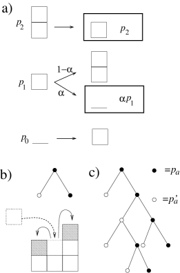
Figure 1: Illustration of the branching process. In a) the processes following a grain drop are depicted. Original configurations and their probabilities are in the left column, final ones in the right column. The possible final configurations resulting from a toppling are framed together with their non-normalized probabilities. In b) the correspondence is shown between one branching event and the toppling, in which one new grain is added and two grains (shaded) are displaced to the left and to the right from the toppling site. In c) a sample realization of the tree is sketched. The full circles placed on the right-hand branches correspond to probabilities $p_{a}$, while empty circles on the left-hand branches have modified probabilities $p^{\prime}_{a}$.

The root of the tree should be treated separately. The reason is that in the ricepile model the avalanche starts by dropping a grain always on the left edge of the pile, i. e. on the site $i=1$. If it topples, it transfers a grain only to the right, while the grain going left falls off the system. If we translated this feature to the description of our branching process, the root would consist either of a single non-branching point, or a point with a single branch (the right one) emerging from it. However, we are interested in the regime of long trees, where the different behaviour of the root from the rest of the tree is irrelevant. So, we assume that in the branching process also the root obeys the same rules as all other points. Thus, all points, including the root, have either zero or two branches emanating from it.

The key quantity will be $P_{n}^{a}(s)$, the probability that a tree consisting of $n$ levels starting with a point of type $a$ contains $s$ branchings. The probability of having $s$ branchings (i. e. avalanche of size $s$) is then $P_{n}(s)=\sum_{a}\;p_{a}P_{n}^{a}(s)$. We can easily derive the recurrence relation for $P_{n}^{a}(s)$ which becomes particularly simple if we use the characteristic function. We obtain

$$\hat{P}_{n}^{a}(\zeta)=(1-q_{a})+q_{a}\zeta\sum_{b,c=0}^{2}p_{b}p^{\prime}_{c}\hat{P}_{n-1}^{b}(\zeta)\hat{P}_{n-1}^{c}(\zeta)\;\;.$$ (3)

A straightforward calculation leads to the following equations for the characteristic functions

$$\begin{split}\hat{P}^{0}_{n}(\zeta)&=1\\ \hat{P}^{1}_{n}(\zeta)&=1-\alpha+\alpha\hat{P}^{2}_{n}(\zeta)\end{split}$$ (4)

and

$$P_{n}(s)=(\alpha p_{1}+p_{2})P^{2}_{n}(s)\;\;{\rm for}\;s>0\;\;.$$ (5)

Therefore the basic quantity of interest will be the characteristic function $\hat{P}^{2}_{n}(\zeta)$. All properties of the branching process can be computed from it. The set of equations (3) thus represent a single recurrence equation for $\hat{P}^{2}_{n}(s)$, which in the limit $n\to\infty$ leads to quadratic equation for the stationary distribution $\hat{P}^{2}(\zeta)=\lim_{n\to\infty}\hat{P}^{2}_{n}(\zeta)$. We obtain explicitly

$$\begin{split}\frac{1}{\zeta}&\,\hat{P}^{2}(\zeta)=\\ &{\frac{\left(\alpha\,p_{{1}}+(1-\alpha)p_{{2}}\right)\left(1-\alpha\,p_{{1}}-p_{{2}}\right)}{p_{{2}}+\alpha\,p_{{1}}}}+\\ &+{\frac{\alpha\,p_{{2}}+2\,\alpha\,(1-\alpha)\,p_{{1}}p_{{2}}+(1-2\alpha)\,{p_{{2}}}^{2}+{p_{{1}}}^{2}{\alpha}^{2}}{p_{{2}}+\alpha\,p_{{1}}}}\hat{P}^{2}(\zeta)\\ &+\alpha\,p_{{2}}(\hat{P}^{2}(\zeta))^{2}\quad.\end{split}$$ (6)

2.4 Criticality

The discriminant $D(\zeta)$ of the equation (6) depends on the parameters $p_{1}$, $p_{2}$, and $\alpha$. The branching process is critical if $D(1)=0$. This implies the following relation

$$-\alpha\,p_{{1}}-(1-\alpha)\,p_{{2}}+2\,\alpha\,p_{{1}}p_{{2}}+{p_{{1}}}^{2}{\alpha}^{2}+{p_{{2}}}^{2}=0$$ (7)

which determines a surface in the parametric space. On this surface the process is critical and the distribution of avalanche sizes has a power-law tail with exponent $\tau=3/2$.

However, the latter statement is not strictly true in the sense that if the coefficient at the quadratic term in the equation (6) is zero, the process is not a true branching process, because each parent can have at most one offspring. It corresponds to a process with an exponential distribution of avalanche sizes, which we will call, in this work, a “one-dimensional BTW process”. The important feature which makes it different from a generic branching process is that there are no true branching points. Indeed, there may be a non-zero probability that the process stops at a given point, but there is zero probability to be split into more than one branch. Therefore, the process does not generate a tree-like structures, but linear chains of random length. Both one-dimensional BTW and branching processes have the same general form (1) of the distribution of avalanches for large $s$, but the one-dimensional BTW process is characterised by the exponents $\tau=0,\;\eta=-1$. Therefore, together with checking the criticality condition (7) we must also look at the behaviour close to the singularity.

We will prove in the section 3.2 that in the thermodynamic limit our ricepile model self-organizes so that the parameters stabilise at values

$$\begin{split}p_{1}=&\max(0,\frac{2\,\alpha-1}{\alpha})\\ p_{2}=&1-\alpha\;\;.\end{split}$$ (8)

If we insert these values into the criticality condition (7), we find that it is satisfied for any value of $\alpha$, including the limit values of 0 and 1. At the same time we find that the singularity is always located at $\zeta_{0}=1$. (Indeed, as we discussed in section 2.2, the criticality of the process is equivalent to the condition $\zeta_{0}=1$.) However, we find that the type of the singularity corresponds to the exponents $\eta=1/2$, $\tau=3/2$ (critical branching process) only for $\alpha$’s within the open interval $(0,1)$, while at the points 0 and 1 the model corresponds to one-dimensional BTW process. This can be easily interpreted in the language of sand- and ricepiles. Indeed, for $\alpha=0$ and $1$ the system recovers the behaviour of one-dimensional BTW sandpile, which does not exhibit critical behaviour in the usual sense. (In fact, the avalanche distribution does exhibit a power-law distribution: all avalanche sizes have the same probability, which corresponds to the power with exponent 0. But this is not the situation we usually describe as critical behaviour.)

2.5 Crossover behaviour

The question arises, how the behaviour with exponent $\tau=3/2$ inside the interval $[0,1]$ crosses over to the exponent $\tau=0$ at the edges. As the critical behaviour is related to the singularities of the characteristic function, we will turn to the investigation of the function $\hat{P}^{2}(\zeta)$ in more detail.

Indeed, we find that if we expand the solution of Eq. (6) for small values of the parameter $\rho$ defined as

$$\rho(\zeta)=\frac{2\,\alpha\,(1-\alpha)}{\zeta^{-1}-1+2\,\alpha\,(1-\alpha)}$$ (9)

we can express the solution in terms of $\rho$ and expand in the lowest order (for $\rho^{2}\ll 1$)

$$\hat{P}^{2}(\zeta)=\frac{1}{\rho}-\sqrt{\frac{1}{\rho^{2}}-1}\simeq\frac{\rho(\zeta)}{2}\;\;.$$ (10)

While, as noted earlier, the exact solution for $\hat{P}^{2}(\zeta)$ has always the singularity of the type $\eta=1/2$ for $\zeta\to\zeta_{0}=1$, the approximate behaviour (10) has a singularity with $\eta=-1$ located at the point $\zeta_{0}^{\prime}=(1-2\,\alpha\,(1-\alpha))^{-1}>1$. When $\alpha$ goes to either 0 or 1, the value of $\zeta_{0}^{\prime}$ approaches 1. This suggests the following scenario. For large avalanches, i. e. $1-\zeta\ll\zeta_{0}^{\prime}-1$ the singularity at $\zeta_{0}=1$ is relevant and the avalanche size distribution has a power-law tail with exponent $\tau=3/2$.

For shorter avalanches, i. e. $1-\zeta$ larger or comparable to $\zeta_{0}^{\prime}-1$ the singularity at $\zeta_{0}^{\prime}$ becomes dominant. Therefore, for short avalanches we have one-dimensional BTW behaviour $P(s)\sim\exp(-s/s_{0})$ with a cutoff

$$s_{0}=|1-\zeta_{0}^{\prime}|^{-1}=\frac{1-2\,\alpha\,(1-\alpha)}{2\,\alpha\,(1-\alpha)}\quad.$$ (11)

The next step is investigation of the behaviour of $s_{0}$ when $\alpha$ approaches either 0 or 1. We find it by expanding the expression for $\zeta_{0}^{\prime}$ as a function of $\alpha$ around the points 0 and 1, respectively. To make the notation more compact, let us introduce the variable $\mu\in\{0,1\}$, which distinguishes the two limit points $\alpha=0$ and 1. We can see from (11) that the cutoff diverges as

$$s_{\rm 0}\simeq\frac{1}{2\,|\alpha-\mu|}$$ (12)

for $\alpha\to\mu$.

On the other hand, sufficiently close to the singularity at $\zeta\to\zeta_{0}=1$ the exponent $\eta=1/2$ is relevant. The question is, how close to $\zeta=1$ one behaviour crosses over to the other. We have one-dimensional BTW behaviour for $\rho^{2}\ll 1$, while critical branching process behaviour for $1-\rho^{2}\ll 1$. A typical crossover value $\zeta_{\rm cr}$ can be found by solving the equation

$$\rho(\zeta_{\rm cr})=\frac{1}{2}\quad.$$ (13)

The avalanche size distribution will exhibit the crossover around $s_{\rm cr}=1/|1-\zeta_{\rm cr}|$. For $s\ll s_{\rm cr}$ the one-dimensional BTW behaviour with exponential cutoff, diverging to infinity for $\alpha=0$ and 1, will apply, while for $s\gg s_{\rm cr}$ the distribution will have power-law tail with usual mean-field exponent $-3/2$, and therefore exhibits self-organized criticality.

The point of the transition between SOC and one-dimensional BTW when $\alpha$ approaches to 1 or 0 lies in the diverging crossover value for the avalanche size. Similarly as in the case of $s_{0}$, by solving the equation (13) with defintition (9) we find the following limit behaviour

$$s_{\rm cr}\simeq\frac{1}{2\,|\alpha-\mu|}\simeq s_{0}$$ (14)

for $\alpha\to\mu$.

We can see, comparing equations (12) and (14), that the cutoff for the one-dimensional BTW behaviour is asymptotically equal to the crossover at which the critical branching process behaviour sets on. This suggests the scaling form

$$P(s)\simeq\frac{1}{s_{0}(\alpha)}\,F(\frac{s}{s_{0}(\alpha)})$$ (15)

valid for $s\gg 1$ and $\alpha$ close to 0 and 1. The scaling function has the form $F(x)\sim\,{\rm e}^{-x}$ for $x\ll 1$ and $F(x)\sim x^{-3/2}$ for $x\gg 1$. Indeed, we can find the Laplace transform of the scaling function as

$$\int_{0}^{\infty}{\rm e}^{-x(y-1)}\,F(x)\,{\rm d}x=y-\sqrt{y^{2}-1}\quad.$$ (16)

From here we obtain immediately the expression for the scaling function through the Bessel function of imaginary argument

$$F(x)=\frac{{\rm e}^{-x}}{x}\,I_{1}(x)\quad.$$ (17)

The expected behaviour for $x\ll 1$ and $x\gg 1$ can be verified directly by inspecting the asymptotic behaviour of the Bessel function.

3 Self-organization

3.1 Self-organized branching process

In the basic setup of our branching process, all three parameters $\alpha$, $p_{1}$, $p_{2}$ are freely chosen. However, in the ricepile model the only free parameter is $\alpha$. The number of sites with given $z$ can change during an avalanche, so that also the probabilities $p_{1}$ and $p_{2}$ are modified. This defines a flow in the space of parameters $p_{1}$, $p_{2}$. Our task now is to establish stable fixed points of this dynamics and check whether they satisfy the condition (7). If that happens, we can conclude that the system is self-organized critical.

There are four types of events, which can happen during an avalanche. Let us denote them $T2$, $T1$, $E1$, $E0$. In the event $T2$, the point with $z=2$ receives a grain and topples. As a result, the number of sites with $z=2$ is decreased by 1, $N_{2}\to N_{2}-1$, and number of sites with $z=1$ is increased by 1, $N_{1}\to N_{1}+1$. Similarly, in the event $T1$ point with $z=1$ topples, $N_{1}\to N_{1}-1$ and $N_{0}\to N_{0}+1$, in event $E1$ site with $z=1$ receives a grain but does not topple, $N_{1}\to N_{1}-1$ and $N_{2}\to N_{2}+1$, and finally in event $E0$ site with $z=0$ receives a grain and does not topple, $N_{0}\to N_{0}-1$ and $N_{1}\to N_{1}+1$.

Using the variables $y\in\{T,E\}$ and $a,b\in\{0,1,2\}$, let us denote $s_{ayb,n}$ the number of events of the type $yb$ occurring at the level $n$ within the branching process, on condition that the very first site had $z=a$. There are $s_{ayb}=\sum_{n=0}^{\infty}s_{ayb,n}$ such events in the entire realisation of the branching process. On average, there are $\langle s_{yb}\rangle=\sum_{a}\,p_{a}\langle s_{ayb}\rangle$ events of the type $yb$. The averages $\langle s_{yb}\rangle$ are of central importance for the dynamics of the self-organization and can be easily obtained as follows.

For the characteristic function of the probability distributionof the number of events $s_{ayb,n}$ we obtain an equation analogical to (3). To study the self-organization, we will need only the average number of events, which is $\langle s_{ayb,n}\rangle$, calculated as derivative of the characteristic function. Hence

$$\langle s_{ayb,n}\rangle=q_{a}\sum_{c}(p_{c}+p_{c}^{\prime})\langle s_{cyb,n-1}\rangle\quad.$$ (18)

This is a set of three recurrence relations, which may be reduced to one equation only, by considering the relations $\langle s_{0yb,n}\rangle=0$ and $\langle s_{1yb,n}\rangle=\alpha\,\langle s_{2yb,n}\rangle$, valid for $n>1$. If we take as the basic quantity the average $\langle s_{2yb,n}\rangle$, we get a recurrence relation determining a geometric sequence

$$\langle s_{2yb,n+1}\rangle=\kappa\langle s_{2yb,n}\rangle$$ (19)

with quotient

$$\kappa=\frac{\alpha\,p_{2}+(p_{2}+\alpha\,p_{1})^{2}}{p_{2}+\alpha\,p_{1}}\quad.$$ (20)

We recognise in the stationarity condition $\kappa=1$ the equation (7), implying the criticality of the branching process.

Summation of the infinite geometric series gives immediately

$$\langle s_{yb}\rangle=\left(p_{b}+(p_{b}+p_{b}^{\prime})\frac{\alpha\,p_{1}+p_{2}}{1-\kappa}\right)\langle s_{byb,1}\rangle$$ (21)

where the initial conditions are given by $\langle s_{bTb,1}\rangle=q_{b}$ and $\langle s_{bEb,1}\rangle=1-q_{b}$.

The self-organization of the branching process is due to the changes in the numbers $N_{a}$, caused by the toppling (and non-toppling) events. These numbers determine the probabilities $p_{a}$. Therefore, for fixed $\alpha$ the self-organized branching process (SOBP) ${\cal S}(\alpha)$ consists of an (infinite) sequence of branching processes

$${\cal S}(\alpha)=$$ (22)

$$=[{\cal B}(\alpha,p_{1}^{(0)},p_{2}^{(0)}),{\cal B}(\alpha,p_{1}^{(1)},p_{2}^{(1)}),{\cal B}(\alpha,p_{1}^{(2)},p_{2}^{(2)}),\ldots]$$

where ${\cal B}(\alpha,p_{1},p_{2})$ is the branching process determined by fixed parameters $\alpha,p_{1},p_{2}$, defined above. The branching processes within the sequence differ only by the values of the parameters $p_{1}$, and $p_{2}$. Let us consider the $t$-th branching process in the sequence. When realised, it changes the original values of the numbers $N_{a}$, or, equivalently, the values of the parameters $p_{a}$. The average change is uniquely determined by the average number of events $\langle s_{yb}\rangle$ . So, the SOBP is entirely determined by the transition relations connecting the values of the parameters in the $t$-th and $t+1$-st step

$$p_{i}^{(t+1)}-p_{i}^{(t)}=T_{i}(p_{1}^{(t)},p_{2}^{(t)})$$ (23)

for $i\in\{1,2\}$. We find explicitly

$$\begin{split}&T_{1}(p_{1},p_{2})=\\ &\frac{\alpha p_{1}+(1-\alpha)p_{2}-\alpha(2-\alpha)p_{1}^{2}-p_{2}^{2}-2(1-\alpha)p_{1}p_{2}}{\alpha p_{1}+(1-\alpha)p_{2}+2\alpha p_{1}p_{2}+p_{2}^{2}+\alpha^{2}p_{1}^{2}}\\ &T_{2}(p_{1},p_{2})=\\ &\qquad\frac{\alpha(1-\alpha)p_{1}^{2}+(1-2\alpha)p_{1}p_{2}}{\alpha p_{1}+(1-\alpha)p_{2}+2\alpha p_{1}p_{2}+p_{2}^{2}+\alpha^{2}p_{1}^{2}}\quad.\end{split}$$ (24)

3.2 Fixed point

The fixed point of the self-organization dynamics can be found immediately by equating the right-hand sides of equations (24) to zero. Direct solution of the two coupled equations gives three fixed points

$$p_{1}= 0,\; p_{2}=0$$ (25)

$$p_{1}= 0,\; p_{2}=1-\alpha$$ (26)

$$p_{1}= \frac{2\alpha-1}{\alpha},\; p_{2}=1-\alpha\quad.$$ (27)

The correct solution is determined by stability considerations. The relations (24) are linearised around the fixed points and the eigenvalues of the resulting matrices of rank 2 are found. The result is that the fixed point (25) is always unstable, while (26) is stable for $\alpha\in[0,1/2)$ and (27) is stable for $\alpha\in(1/2,1]$. For $\alpha=1/2$ the fixed points (26) and (27) coincide and both of them are marginally stable (i. e. the eigenvalues have zero real part).

Therefore, we find that the fixed point corresponds to the values of the probabilities

$$\begin{split}p_{1}=&\max\,(0,\frac{2\,\alpha-1}{\alpha})\\ p_{2}=&1-\alpha\end{split}$$ (28)

which proves the already announced result of Eq.(8).

3.3 Finite-size effects

In the numerical simulations of the ricepile model be_be_mhi_zha_99 ; be_be_ke_lo_mhi_99 ; markosova_00 ; markosova-unpublished attention is paid to the fact that the critical behaviour is observed only for large enough systems with $\alpha$ not too close to neither 0 nor 1. We have already shown how the crossover length blows up when $\alpha$ approaches the edge values 0 or 1. It is obvious then, that for small systems the crossover value of the avalanche size may not be accessible and the critical regime in the tail of the distribution is not observed at all. In this subsection we will investigate the consequences of finite length of the branching process. There are two phenomena where the finite size enters the problem. First, if the maximum number of generations in the branching process is $L$, instead of infinity, the distribution of the avalanche sizes will not extend to infinity either, but will be bounded by $s<s_{\rm max}=2^{L}-1$. Moreover, if we take for example $p_{1}=1$, $p_{2}=0$, $\alpha=1$, then all avalanches will have size $L$, therefore a peak at $s=L$ will occur, $P(s)=\delta(s-L)$. If we move slightly from this position by increasing $p_{2}$ and decreasing $p_{1}$ and $\alpha$, a structure of multiple peaks located at $s=L,2L-1,3L-3,...$ will appear. This makes the analysis very complicated.

Second consequence is the shift in the self-organized value of the parameters $p_{1}$ and $p_{2}$, which for finite $L$ will deviate from the critical values. Therefore, the avalanche-size distribution will develop an exponential cutoff in the form $P(s)\propto s^{-3/2}\exp(-s/s_{1})$.

As the first problem brings new particular difficulties, we will concentrate only on the second one. This makes the analysis less consistent, but feasible. Thus, we should stress that in the following we will suppose that the branching process in question has unbounded length, but the self-organization is made in such a way, that only the first $L$ generations of the branching process are taken into account.

Instead of working with finite-$L$ version of the equations (23) and (24), describing the approach to the fixed point, we can use the set of equations

$$\begin{split}\langle s_{E1}\rangle\,=&\,\langle s_{T2}\rangle\\ \langle s_{E0}\rangle\,=&\,\langle s_{T1}\rangle\end{split}$$ (29)

which determine the position of the fixed point. The only information lost in Eq. (29) is the stability of the fixed points. However, we suppose the stability will not be affected by the finite-size effects. Therefore, we will rely on the stability analysis performed for $L=\infty$ also in the case of finite $L$ and calculate the finite-size corrections starting with Eq. (29).

The point is that the equations (29) should hold also for finite $L$. In fact, the expression (21) for the averages $\langle s_{yb}\rangle$ assume the same form, only the factor $(\kappa-1)$ arising in the $L=\infty$ version should be replaced by the factor $K=(\kappa-1)/(\kappa^{L-1}-1)$. Assuming $K$ small for large $L$, we can find $p_{1}$ and $p_{2}$ in lowest order in $K$. Then, we return to the definition of $K$ and find that $K\propto L^{-1}$, confirming that our approach is consistent.

Hence, for finite $L$ we find, by solving the equations (29) to lowest order in $1/L$, for $\alpha\in(0,1/2)$

$$\begin{split}p_{1}&=-\frac{1-\alpha}{(2\alpha-1)^{2}}\;\frac{\ln(1-\gamma)}{L}+O(\frac{1}{L^{2}})\\ p_{2}&=1-\alpha-\frac{1-\alpha}{2\alpha-1}\;\frac{\ln(1-\gamma)}{L}+O(\frac{1}{L^{2}})\end{split}$$ (30)

and for $\alpha\in(1/2,1)$

$$\begin{split}p_{1}&=\frac{2\alpha-1}{\alpha}+\frac{5\alpha^{2}-5\alpha+1}{(2\alpha-1)^{2}\,\alpha}\;\frac{\ln(1-\gamma)}{L}+O(\frac{1}{L^{2}})\\ p_{2}&=1-\alpha+\frac{1-\alpha}{2\alpha-1}\;\frac{\ln(1-\gamma)}{L}+O(\frac{1}{L^{2}})\end{split}$$ (31)

where we denoted

$$\begin{split}\gamma&=\frac{1}{2}\frac{1-2\alpha}{1-\alpha}\quad{\rm for}\quad\alpha\in(0,1/2)\\ \gamma&=\frac{1}{2}\frac{2\alpha-1}{\alpha}\quad{\rm for}\quad\alpha\in(1/2,1)\quad.\end{split}$$ (32)

The above formulae confirm that the explicit limit $L\to\infty$ gives the same result as obtained previously when working directly with $L=\infty$.

Using these results we can find the position of the square-root singularity in the characteristic function for the avalanche size distribution, solving the equation$D(\zeta_{0})=0$. The distance from 1 then determines the exponential cutoff of the distribution. We find

$$1/s_{1}=|\zeta_{0}-1|=\frac{\sigma(\alpha)}{L^{2}}+O(\frac{1}{L^{3}})$$ (33)

where

$$\sigma(\alpha)=\frac{\ln^{2}(1-\gamma)}{4\,\alpha\,(1-\alpha)}\quad{\rm for}\quad\alpha\in(0,1)$$ (34)

and asymptotically for $L\to\infty$ and $\alpha$ fixed the avalanche distribution becomes the function of $s\,L^{-2}$ only,

$$P(s;\alpha,L)\propto L^{-3}\,G(sL^{-2}\,\sigma(\alpha))$$ (35)

and he scaling function has the form

$$G(x)=x^{-3/2}{\rm e}^{-x}\quad.$$ (36)

This scaling holds well for all $\alpha$ with exception of the point $\alpha=1/2$, where we have $\gamma=0$ and hence $\sigma(\alpha)=0$. Then, the next order in $1/L$ takes over and the scaling changes.

Let us use again the variable $\mu\in\{0,1\}$, which distinguishes the two limit points $\alpha=0$ and 1. The factor $\sigma(\alpha)$ diverges as $\sigma(\alpha)\simeq\sigma_{0}\,|\alpha-\mu|^{-1}$ for $\alpha\to\mu$, where $\sigma_{0}=(\ln 2)^{2}/4$. Therefore, we can write the following scaling form for the avalanche size distribution

$$P(s;\alpha,L)\propto L^{-3}|\alpha-\mu|^{-\frac{3}{2}}\,G(s\,L^{-2}|\alpha-\mu|^{-1}\,\sigma_{0})$$ (37)

for $\alpha\to\mu$.

We can see that the power-law distribution holds only for avalanches shorter than $L^{2}\,|\alpha-\mu|$. In other words, if the parameter $\alpha$ is close to the end-points of the interval $[0,1]$, we need to have systems of the size $L\gg 1/\sqrt{|\alpha-\mu|}$ for being able to observe any sign of self-organized criticality.

In the above calculations we tacitly assumed that we beyond the regime we called “one-dimensional BTW” in the section 2.5. This means $s\gg s_{\rm cr}$. In fact, we can always reach this regime by choosing $L$ large enough. Therefore the presence of the one-dimensional regime does not influence the scaling behaviour for large $L$. More precisely, we should have $L^{2}\,|\alpha-\mu|\gg s_{\rm cr}$. But because $s_{\rm cr}$ itself diverge for $\alpha\to\mu$ as $|\alpha-\mu|^{-1}$, we obtain a stronger condition for the scaling (37) to be valid, namely

$$L\gg|\alpha-\mu|^{-1}$$ (38)

if $\alpha\to\mu$.

4 Conclusions

We investigated analytically the self-organized critical ricepile model. We defined a self-organized branching process, suitable for one-dimensional problems. The model is characterised by the parameter $\alpha\in[0,1]$, the probability of toppling at a sub-threshold site. For both limit values $\alpha=0$ and $\alpha=1$ the model is equivalent to the one-dimensional BTW model with trivial (uniform) distribution of avalanches.

We found that in the thermodynamic limit the system is self-organized critical for all values of $\alpha$ within the open interval $(0,1)$, with power-law tail in the distribution of avalanche sizes with mean-field value of the exponent, $\tau=\frac{2}{3}$. However, the power-law behaviour holds only for avalanches longer than a certain crossover value of the avalanche size. The crossover diverges when $\alpha$ approaches to either of the limit points of the interval $[0,1]$. We found the scaling as well as the exact form of the scaling function for avalanche distribution close to these limit points. This describes how the one-dimensional BTW behaviour develops when approaching the limit points.

The finite-size effects play important role in determining whether the model is self-organized critical or not. In our model the SOC behaviour starts to occur at the larger sizes the closer we are to the limit points $\alpha=0$ or $1$. We found the form of the finite size scaling in our self-organized branching process and determined the necessary condition for the the power-law regime in the avalanche distribution to be observable, when we approach to the limit points.

- (1) P. Bak, C. Tang, and K. Wiesenfeld, Phys. Rev. Lett. 59, 381 (1987).
- (2) P. Bak, C. Tang, and K. Wiesenfeld, Phys. Rev. A 38, 364 (1988).
- (3) L. P. Kadanoff, S. R. Nagel, L. Wu, and S.-M. Zhou, Phys. Rev. A 39, 6524 (1989).
- (4) P. Grassberger and S. S. Manna, J. Phys. France 51, 1077 (1990).
- (5) S. S. Manna, Physica A 179, 249 (1991).
- (6) S. S. Manna, J. Phys. A: Math. Gen. 24, L363 (1991).
- (7) A. Chessa, H. E. Stanley, A. Vespignani, and S. Zapperi, Phys. Rev. E 59, R12 (1999).
- (8) D. Sornette, A. Johansen, and I. Dornic, J. Phys. I France 5, 325 (1995).
- (9) K. Wiesenfeld, J. Theiler, and B. McNamara, Phys. Rev. Lett. 65, 949 (1990).
- (10) M. Markošová and P. Markoš, Phys. Rev. A 46, 3531 (1992).
- (11) P. Helander, S. C. Chapman, R. O. Dendy, G. Rowlands, and N. W. Watkins, Phys. Rev. E 59, 6356 (1999).
- (12) H. M. Jaeger, C.-H. Liu, and S. R. Nagel, Phys. Rev. Lett. 62, 40 (1989).
- (13) J. Rajchenbach, Phys. Rev. Lett. 65, 2221 (1990).
- (14) G. A. Held, D. H. Solina, D. T. Keane, W. J. Haag, P. M. Horn, and G. Grinstein, Phys. Rev. Lett. 65, 1120 (1990).
- (15) S. R. Nagel, Rev. Mod. Phys. 64, 321 (1992).
- (16) C. P. C. Prado and Z. Olami, Phys. Rev. A 45, 665 (1992).
- (17) G. C. Baker and A. Mehta, Phys. Rev. E 53, 5704 (1996).
- (18) G. Baumann and D. E. Wolf, Phys. Rev. E 54, R4504 (1996).
- (19) V. Frette, K. Christensen, A. Malte-Sørenssen, J. Feder, T. Jøssang, and P. Meakin, Nature 379, 49 (1996).
- (20) A. Malthe-Sørenssen, J. Feder, K. Christensen, V. Frette, and T. Jøssang, Phys. Rev. Lett. 83, 764 (1999).
- (21) A. Mehta and G. C. Barker, Europhys. Lett. 27, 501 (1994).
- (22) A. Malthe-Sørenssen, Phys. Rev. E 54, 2261 (1996).
- (23) S. Lübeck and K. D. Usadel, Fractals 1, 1030 (1993) (cond-mat/9807021).
- (24) R. Dickman, M. Alava, M. A. Muñoz, J. Peltola, A. Vespignani, and S. Zapperi, cond-mat/0101381.
- (25) V. B. Priezzhev, E. V. Ivashkevich,1, A. M. Povolotsky, and C.-K. Hu, Phys. Rev. Lett. 87, 084301 (2001).
- (26) S. Maslov, C. Tang, and Y.-C. Zhang, Phys. Rev. Lett. 83, 2449 (1999).
- (27) L. A. N. Amaral and K. B. Lauritsen, Phys. Rev. E 54, R4512 (1996).
- (28) L. A. N. Amaral, K. B. Lauritsen, Physica A 231, 608 (1996).
- (29) L. A. N. Amaral and K. B. Lauritsen, Phys. Rev. E 56, 231 (1997).
- (30) K. Christensen, A. Corral, V. Frette, J. Feder, and T. Jøssang, Phys. Rev. Lett. 77, 107 (1996).
- (31) M. Paczuski and S. Boettcher, Phys. Rev. Lett. 77, 111 (1996).
- (32) S.-D. Zhang, Phys. Lett. A 233, 317 (1997).
- (33) M. Bengrine, A. Benyoussef, F. Mhirech, and S. D. Zhang, Physica A 272, 1 (1999).
- (34) M. Bengrine, A. Benyoussef, A. El Kenz, M. Loulidi, and F. Mhirech, Eur. Phys. J. B 12, 129 (1999).
- (35) M. Markošová, M. H. Jensen, K. B. Lauritsen, and K. Sneppen, Phys. Rev. E 55, R2085 (1997).
- (36) M. Markošová, Phys. Rev. E 61, 253 (2000).
- (37) S.-D. Zhang, Phys. Rev. E 61, 5983 (2000).
- (38) P. M. Gleiser, S. A. Cannas, F. A. Tamarit, and B. Zheng, Phys. Rev. E 63, 042301 (2001).
- (39) P. M. Gleiser, Physica A 295, 311 (2001).
- (40) D. Dhar and R. Ramaswamy, Phys. Rev. Lett. 63, 1659 (1989).
- (41) D. Dhar and S. N. Majumdar, J. Phys. A: Math. Gen. 23, 4333 (1990).
- (42) M. Markošová, J. Phys. A: Math. Gen. 28, 6903 (1995).
- (43) M. Kloster, S. Maslov, and C. Tang, Phys. Rev. E 63, 026111 (2001).
- (44) L. Pietronero, A. Vespignani, and S. Zapperi, Phys. Rev. Lett. 72, 1690 (1994).
- (45) E. V. Ivashkevich, Phys. Rev. Lett. 76, 3368 (1996).
- (46) Y.-C. Zhang, Phys. Rev. Lett. 63, 470 (1989).
- (47) C. Tang and P. Bak, J. Stat. Phys. 51, 797 (1988).
- (48) K. Kawasaki and T. Koga , Physica A 224, 1 (1996).
- (49) A. Vespignani and S. Zapperi, Phys. Rev. E 57, 6345 (1998).
- (50) P. Alstrøm, Phys. Rev. A 38, 4905 (1988).
- (51) R. García-Pelayo, Phys. Rev. E 49, 4903 (1994).
- (52) S. Zapperi, K. B. Lauritsen, and H. E. Stanley, Phys. Rev. Lett. 75, 4071 (1995).
- (53) K. B. Lauritsen, S. Zapperi, and H. E. Stanley, Phys. Rev. E 54, 2483 (1996).
- (54) G. Caldarelli, C. Tebaldi, and A. L. Stella, Phys. Rev. Lett. 76, 4983 (1996).
- (55) M. Vergeles, A. Maritan, and J. R. Banavar, Phys. Rev. E 55, 1998 (1997).
- (56) J. Chu and C. Adami, cond-mat/9903085.
- (57) J. Chu and C. Adami, Proc. Nat. Acad. Sci. 96, 15017 (1999).
- (58) O. Sotolongo-Costa, A. Vazquez, and J. C. Antoranz, Phys. Rev. E 59, 6956 (1999).
- (59) H. F. Ouyang, Y. N. Lu, and E. J. Ding, Phys. Rev. E 48, 2413 (1993).
- (60) M. Markošová, (unpublished).