Crystallographic Method for Exact Describing Quasicrystal Structures

In this paper the problem of the theory of a quasicrystal structures - the determination of coordinates of each atom of quasicrystal in analytical form - is solved. Within the framework of the proposed model a periodic crystal can be presented as a particular case of a quasicrystal. The simple and explicit analytical formulas which describe the location of each atom in a quasicrystal are given. The exact solutions for Penrose and Ammann-Beenker quasicrystal structures are given. On the basis of the analytical formulas the routines are created. The routines are inserted directly into graphical files generating the quasiperiodic structures.

1 Introduction

Since quasicrystals were discovered [1] quasiperiodic structures have been widely studied, see e.g. [3-14]. The two standard ways to describe these structures are the cut and project method [3-7], and the grid algorithm [8-10]. However the basic unsolved problem of the theories of quasicrystals was the problem: the determination of true atom locations in a quasicrystal [2]. The solution of this problem is given in this paper. To solve the specified problem a method has been applied, which includes traditional crystallography, which describes periodic and incommensurate crystalline structures. The symmetries of quasicrystal structures are considered with the superspace-groups [15, 16], which are the classical method of describing incommensurate structures now.

2 Quasicrystal structures

Structures, in particular quasicrystals, which form point diffraction patterns, but aren’t periodic, can be described by the finite number of structural cells. The scheme for a two-dimensional quasicrystal with structural cells $\mathbf{a}$–$\mathbf{w}$ is given on fig. 1.

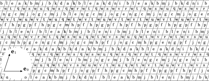
Fig. 1: The scheme of two-dimensional quasicrystal with structural cells $\mathbf{a}$–$\mathbf{w}$.

In such a quasicrystal with crystallographic axes, parallel $\mathbf{e}_{0}$, $\mathbf{e}_{1}$, structural cells are located in the nodes of the quasiperiodic lattice with the coordinates

$$\mathbf{r_{n}}(\boldsymbol{\alpha,\beta})=\mathbf{e}_{0}\,x_{n_{0}}\!(\alpha_{0},\beta_{0})+\mathbf{e}_{1}\,x_{n_{1}}\!(\alpha_{1},\beta_{1}),$$ (1)

where $x_{n_{l}}=a_{l}\left(n_{l}+\alpha_{l}+1/\chi_{l}\left\lfloor(n_{l}+\beta_{l})/\sigma_{l}\right\rfloor\right)$, $\lfloor{x}\rfloor$ – is the greatest integer part not exeeding $x$, $\sigma_{l}>1$ and $\chi_{l}$ – irrational numbers, $\alpha_{l}$ and $\beta_{l}$ – arbitrary numbers, $a_{l}$ – the parameters of the lattice, $l=0,1$. Further we will consider $\beta_{l}\left/\sigma_{l}\right.<1$, since in the opposite case $\alpha$ changes, i.e. $\alpha_{l}^{\prime}=\alpha_{l}+1/\chi_{l}{\left\lfloor{\beta_{l}/\sigma_{l}}\right\rfloor}$. Introduce a vector $\boldsymbol{\Upsilon}_{\mathbf{n}}(\boldsymbol{\beta})$ in the Cartesian coordinates:

$$\boldsymbol{\Upsilon}_{\mathbf{n}}(\boldsymbol{\beta})=\left(\sigma_{0}\!\left\{\frac{n_{0}+\beta_{0}}{\sigma_{0}}\right\},\;\sigma_{1}\!\left\{\frac{n_{1}+\beta_{1}}{\sigma_{1}}\right\}\right),$$ (2)

where $\{x\}$ – the fractional part of $x$. Then the atom density distribution for quasicrystal with $K$ structural cells can be written in the form

$$\rho(\mathbf{n},\boldsymbol{\alpha},\boldsymbol{\beta})= \sum_{n_{0},\,n_{1}=-\infty}^{\infty}\sum_{k=1}^{K}p_{k}(\mathbf{n}+\boldsymbol{\beta})\sum_{j_{k}=1}^{J_{k}}\delta(\mathbf{r-r_{n}(\boldsymbol{\alpha},{\boldsymbol{\beta}})-r}_{j_{k}}),$$ (3)

$$p_{k}(\mathbf{n}+\boldsymbol{\beta}) =\left|\begin{array}[]{rr}1,&\;\>\boldsymbol{\Upsilon}_{\mathbf{n}}(\boldsymbol{\beta})\in{U_{k}},\\ 0,&\;\boldsymbol{\Upsilon}_{\mathbf{n}}(\boldsymbol{\beta})\notin{U_{k}},\end{array}\right.$$ (6)

where ${\mathbf{r}_{j}}_{k}$ is a vector, determining the location of the atom centres of the structural cell with the index $k$ relative to the nodes of the lattice, to which the cell is related, the areas $U_{k}$ are placed in a rectangle $\sigma_{0}\times\sigma_{1}$. In general case the area $U_{k}$ will be an arbitrary form (fig. 2).

Fig. 2: In the area of U_k, corresponding structural cell with the index $k$, the condition $p_{k}(\mathbf{n}+\boldsymbol{\beta})=1$ is true.

The area U_k can be defined if to compute $\sim$ 100 $\div$ 200 points ${\boldsymbol{\Upsilon}}_{\mathbf{n}}(\boldsymbol{\beta})$ for each structural cell. Equations (3) and (4) define the atom locations of the quasicrystal and can be easily inserted into routine to generate quasicrystal structures of any size with arbitrary parameters $\boldsymbol{\alpha}$, $\boldsymbol{\beta}$. As an example we’ll present the solution for quasicrystals of Penrose [17] ($\sigma_{0}\!=\!\sigma_{1}\!=\!\chi_{0}\!=\!\chi_{1}\!=\!\tau$, $\tau\!=\!(1+\sqrt{5})/2$, $a_{0}\!=\!a_{1}\!=\!1$) and Ammann-Beenker [18, 19] ($\sigma_{0}\!=\!\sigma_{1}\!=\!\chi_{0}\!=\!\chi_{1}\!=a_{0}\!=\!a_{1}\!=\!\sigma$, $\sigma\!=\!1+\sqrt{2}$ ) (fig.3). The analytical formulas of areas $U_{k}$ given in appendix. On the fig. 4 superposition of two Penrose quasicrystals with different parameters $\boldsymbol{\beta}$ is presented. The routine by formulas (3) and (4) is inserted directly into graphical file generating fig. 4 and parameters $\boldsymbol{\beta}$ change randomly for each loading the figure so one can observe phason [20-23] flips in real time zooming screen or loading several windows.

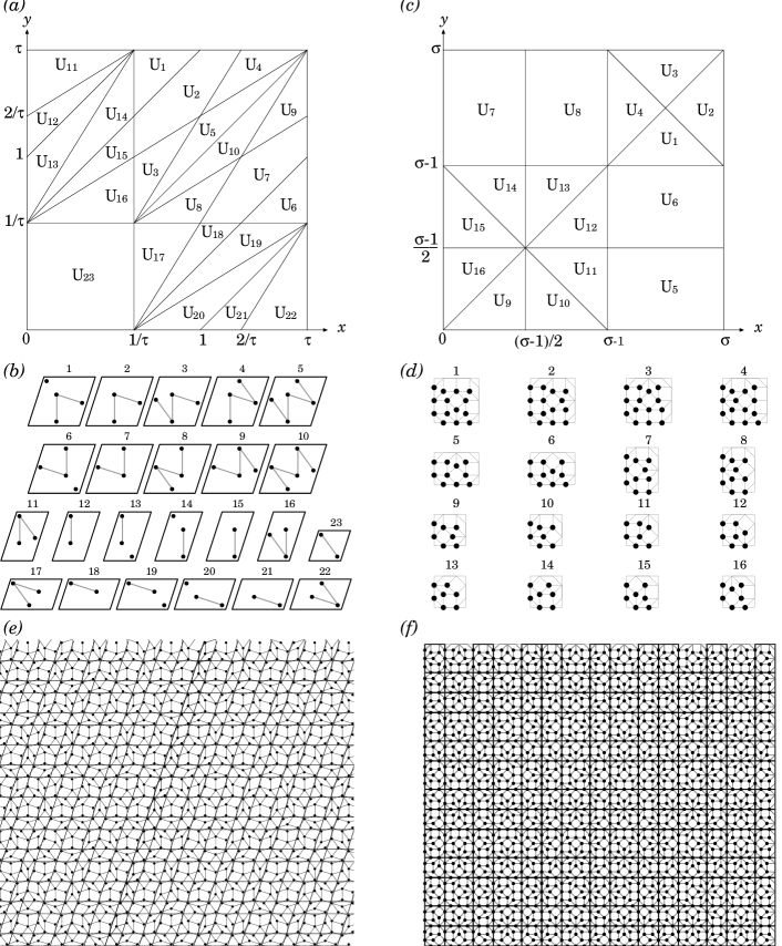
Fig. 3: In the upper left part of the figure $(a)$ the card of the areas U_k and corresponding $(b)$ 23 structural cells for the Penrose quasicrystal are placed, in the right upper part – a similar scheme $(c)$, $(d)$ for the Ammann-Beenker quasicrystal with sixteen structural cells. The quasicrystals $(e)$, $(f)$ in the lower part of the figure are generated by the computer program based on formulas (3), (4) and schemes $(a)$, $(b)$ and $(c)$, $(d)$ correspondingly. The analytical formulas of areas $U_{k}$ for the cards $(a)$, $(c)$ given in appendix.

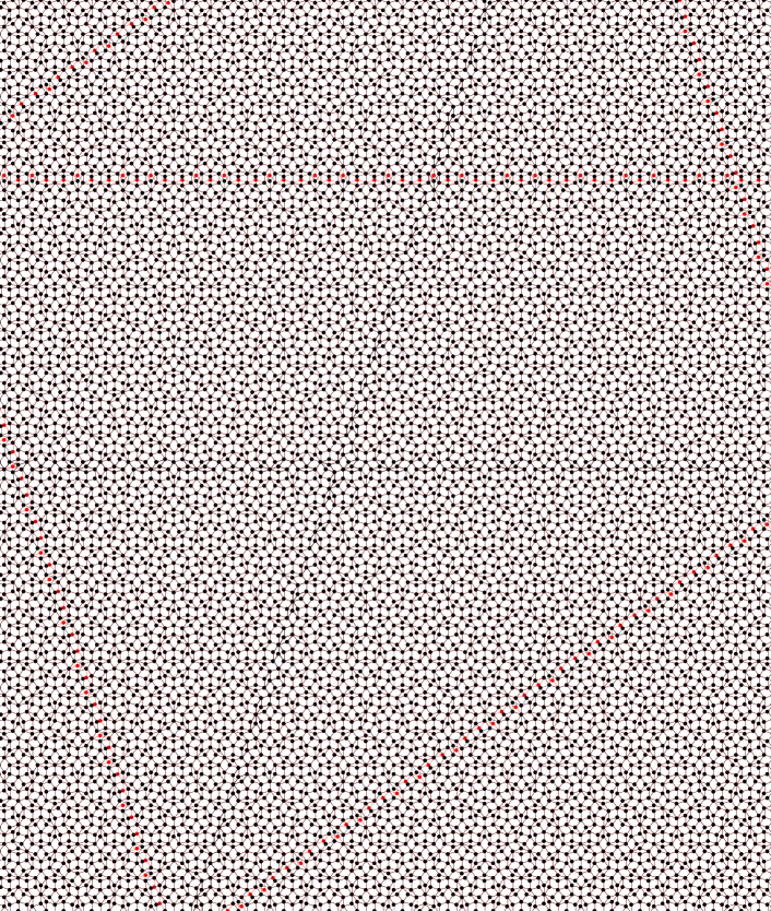
Fig. 4: Phason flips in real time. The routine by formulas (3) and (4) is inserted directly into graphical file generating fig. 4 and parameters $\boldsymbol{\beta}$ change randomly for each loading the figure so one can observe phason flips zooming screen or loading several windows. (This file must be $\ast$.ps not $\ast$.pdf)

The method of describing quasicrystal structures was for demonstration presented on the plane. In the three–dimensional space the structural cells will be parallelepipeds with ribs, which are parallel with the crystallographic axes, the areas U_k will be the elements of volume in a rectangular parallelepiped $\sigma_{0}\times\sigma_{1}\times\sigma_{2}$. For the first time this approach is proposed in [24], the exact solution for the quasicrystal of Penrose given in [25].

3 Rotational symmetries

Analytical calculation [25] of diffraction radiating by formula (3) and (4) for the arbitrary form of the areas U_k shows that the diffraction patterns do not depend on the parameters $\boldsymbol{\alpha}$ and $\boldsymbol{\beta}$. Since the physical property of a quasicrystal, radiation scattering, is independent on $\boldsymbol{\alpha}$ and $\boldsymbol{\beta}$, the condition of invariance for quasicrystal will be the following [15, 16]: if under the operator influence of the transformation on the atom density distribution $\rho(\mathbf{r},\boldsymbol{\alpha},\boldsymbol{\beta})$ only the $\boldsymbol{\alpha}$ and $\boldsymbol{\beta}$ parameters change, but not the $\rho$ function itself then the quasicrystal is invariant in respect to such a transformation. Thus, if for the quasicrystal the following condition holds true

$$R(2\pi/q,\mathbf{r}_{0})\rho(\mathbf{r},\boldsymbol{\alpha},\boldsymbol{\beta})=\rho(\mathbf{r},\boldsymbol{\alpha}^{\,\prime},\boldsymbol{\beta}^{\,\prime}),$$ (7)

where $R(\varphi,\mathbf{r}_{0})$ – the rotation operator, $\varphi$ – the corner of rotation, $\mathbf{r}_{0}$ – is the point coordinate, around which the rotation is performed, then such a quasicrystal will have the symmetry axis of the $q$ order (Fig. 5).

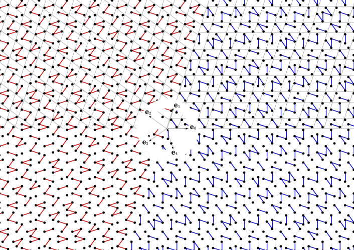
Fig. 5: Illustration of symmetry on the example of the Penrose quasicrystal. In the coordinate bases $\mathbf{e}_{1},\mathbf{e}_{2}$ and $\mathbf{e}_{0},\mathbf{e}_{1}$ the quasicrystal will be described by formulas (3), (4) but with different parameters $\boldsymbol{\alpha}$ and $\boldsymbol{\beta}$.

4 Conclusion

To describe quasicrystals, in contrast to periodic crystals, use is made of a concept on qyasicrystals as objects consisting of several structural units with ribs, which are parallel with crystallographic axes and having a quasiperiodic ordering. It is due to the quasiperiodic ordering of structural units that symmetries, different from classical, are permissible for quasicrystals. Such approach gives simple and explicit analytical formulas which describe the location of each atom in a quasicrystal.

Appendix Appendix A The analytical formulas of areas $U_{k}$ for the Penrose quasicrystal

Designations $x=\tau\{(n_{0}+\beta_{0})/\tau\}$, $y=\tau\{(n_{1}+\beta_{1})/\tau\}$ are used hereinafter.

$$U_{1}=\bigl{(} x\geqslant 1/\tau\bigr{)}\cap\bigl{(}y<\tau\bigr{)}\cap\bigl{(}y>x+1/\tau\bigr{)},$$

$$U_{2}=\bigl{(} x\geqslant 1/\tau\bigr{)}\cap\bigl{(}y<\tau\bigr{)}\cap\bigl{(}y<x+1/\tau\bigr{)}$$

$$\cap\bigl{(}y>x/\tau+1/\tau\bigr{)}\cap\bigl{(}y>\tau x-1/\tau^{2}\bigr{)},$$

$$U_{3}=\bigl{(} x\geqslant 1/\tau\bigr{)}\cap\bigl{(}y<x/\tau+1/\tau\bigr{)}$$

$$\cap\bigl{(}y>\tau x-1/\tau^{2}\bigr{)},$$

$$U_{4}=\bigl{(} y<\tau\bigr{)}\cap\bigl{(}y>x/\tau-1/\tau\bigr{)}$$

$$\cap\bigl{(}y<\tau x-1/\tau^{2}\bigr{)},$$

$$U_{5}=\bigl{(} y>x\bigr{)}\cap\bigl{(}y<x/\tau-1/\tau\bigr{)}$$

$$\cap\bigl{(}y<\tau x-1/\tau^{2}\bigr{)},$$

$$U_{6}=\bigl{(} x<\tau\bigr{)}\cap\bigl{(}y\geqslant 1/\tau\bigr{)}\cap\bigl{(}y<x-1/\tau\bigr{)},$$

$$U_{7}=\bigl{(} x<\tau\bigr{)}\cap\bigl{(}y\geqslant 1/\tau\bigr{)}\cap\bigl{(}y>x-1/\tau\bigr{)}$$

$$\cap\bigl{(}y<x/\tau+1/\tau^{3}\bigr{)}\cap\bigl{(}y>\tau x-1\bigr{)},$$

$$U_{8}=\bigl{(} y\geqslant 1/\tau\bigr{)}\cap\bigl{(}y<x/\tau+1/\tau^{3}\bigr{)}$$

$$\cap\bigl{(}y>\tau x-1\bigr{)},$$

$$U_{9}=\bigl{(} x<\tau)\cap\bigl{(}y>x/\tau+1/\tau^{3}\bigr{)}$$

$$\cap\bigl{(}y<\tau x-1\bigr{)},$$

$$U_{10}\!= \bigl{(}x\!>\!y\bigr{)}\!\cap\!\bigl{(}y\!>\!x/\tau\!+\!1/\tau^{3}\bigr{)}\!\cap\!\bigl{(}y>\!\tau x\!-\!1\bigr{)},$$

$$U_{11}= \bigl{(}x\geqslant 0)\cap(y<\tau\bigr{)}\cap\bigl{(}y>x/\tau+2/\tau\bigr{)},$$

$$U_{12}= (x\!\geqslant\!0\bigr{)}\!\cap\!\bigl{(}y\!<\!x/\tau\!+\!2/\tau\bigr{)}\!\cap\!\bigl{(}y\!>\!x\!+\!1\bigr{)},$$

$$U_{13}= (x\geqslant 0)\cap\bigl{(}y>\tau x+1/\tau\bigr{)}\cap\bigl{(}y<x+1\bigr{)},$$

$$U_{14}= \bigl{(}x\!<\!\tau\bigr{)}\!\cap\!\bigl{(}y\!<\!\tau x\!+\!1/\tau\bigr{)}\!\cap\!\bigl{(}y\!>\!x\!+\!1/\tau\bigr{)},$$

$$U_{15}= \bigl{(}x\!\geqslant\!\tau\bigr{)}\!\cap\!\bigl{(}y\!<\!x\!+\!1/\tau\bigr{)}\!\cap\!\bigl{(}y\!>\!x/\tau\!+\!1/\tau\bigr{)},$$

$$U_{16}= \bigl{(}x\!\geqslant\!1/\tau\bigr{)}\!\cap\!\bigl{(}y\!\geqslant\!1/\tau\bigr{)}\!\cap\!\bigl{(}y\!<\!x/\tau\!+\!1/\tau\bigr{)},$$

$$U_{17}= \bigl{(}y<1/\tau\bigr{)}\cap\bigl{(}x\geqslant\tau\bigr{)}\cap\bigl{(}y>\tau x-1\bigr{)},$$

$$U_{18}= \bigl{(}y\!<\!1/\tau\bigr{)}\!\cap\!\bigl{(}y\!>\!x\!-\!1/\tau\bigr{)}\!\cap\!\bigl{(}y\!<\!\tau x\!-\!1\bigr{)},$$

$$U_{19}= \bigl{(}y\!<\!1/\tau\bigr{)}\!\cap\!\bigl{(}y\!<\!x\!-\!1/\tau\bigr{)}\!\cap\!\bigl{(}y\!<\!x/\tau\!-\!1/\tau^{2}\bigr{)},$$

$$U_{20}= \bigl{(}y\!\geqslant\!0\bigr{)}\cap\bigl{(}y\!>\!x\!-\!1\bigr{)}\cap\bigl{(}y\!<\!x/\tau\!-\!1/\tau^{2}\bigr{)},$$

$$U_{21}= \bigl{(}y\geqslant 0\bigr{)}\cap\bigl{(}y<x-1\bigr{)}\cap\bigl{(}y>\tau x-2\bigr{)},$$

$$U_{22}= \bigl{(}y\geqslant 0\bigr{)}\cap\bigl{(}x<\tau\bigr{)}\cap\bigl{(}y<\tau x-2\bigr{)},$$

$$U_{23}= \bigl{(}0\leqslant x<1/\tau\bigr{)}\cap\bigl{(}0\leqslant y<1/\tau\bigr{)}.$$

Appendix Appendix B The analytical formulas of areas $U_{k}$ for the
Ammann-Beenker quasicrystal

Designations $x=\sigma\{(n_{0}+\beta_{0})/\sigma\}$, $y=\sigma\{(n_{1}+\beta_{1})/\sigma\}$ are used hereinafter.

$$U_{1}= \bigl{(}y\!>\!\sigma\!-\!1\bigr{)}\!\cap\!\bigl{(}y\!<\!x\bigr{)}\!\cap\!\bigl{(}y\!<\!2\sigma\!-\!1\!-\!x\bigr{)},$$

$$U_{2}= \bigl{(}y\!>\!\sigma\!-\!1\bigr{)}\!\cap\!\bigl{(}y\!<\!x\bigr{)}\!\cap\!\bigl{(}y\!>\!2\sigma\!-\!1\!-\!x\bigr{)},$$

$$U_{3}= \bigl{(}y\!>\!\sigma\!-\!1\bigr{)}\!\cap\!\bigl{(}y\!>\!x\bigr{)}\!\cap\!\bigl{(}y\!>\!2\sigma\!-\!1\!-\!x\bigr{)},$$

$$U_{4}= \bigl{(}y\!>\!\sigma\!-\!1\bigr{)}\!\cap\!\bigl{(}y\!>\!x\bigr{)}\!\cap\!\bigl{(}y\!<\!2\sigma\!-\!1\!-\!x\bigr{)},$$

$$U_{5}= \bigl{(}y\leqslant(\sigma-1)/2\bigr{)}\cap\bigl{(}x>\sigma-1\bigr{)},$$

$$U_{6}= \bigl{(}y>(\sigma-1)/2\bigr{)}\cap\bigl{(}x>\sigma-1\bigr{)},$$

$$U_{7}= \bigl{(}x\leqslant(\sigma-1)/2\bigr{)}\cap\bigl{(}y>\sigma-1\bigr{)},$$

$$U_{8}= \bigl{(}x>(\sigma-1)/2\bigr{)}\cap\bigl{(}y>\sigma-1\bigr{)},$$

$$U_{9}= \bigl{(}x>y\bigr{)}\cap\bigl{(}x\leqslant(\sigma-1)/2\bigr{)},$$

$$U_{10}= \bigl{(}x>(\sigma-1)/2\bigr{)}\cap\bigl{(}y<\sigma-1-x\bigr{)},$$

$$U_{11}= \bigl{(}x\!\leqslant\!\sigma\!-\!1\bigr{)}\!\cap\!\bigl{(}y\!>\!\sigma\!-\!1\!-\!x\bigr{)}\!\cap\!\bigl{(}y\!\leqslant\!(\sigma\!-\!1)/2\bigr{)},$$

$$U_{12}= \bigl{(}x\leqslant\sigma-1\bigr{)}\cap\bigl{(}y<x\bigr{)}\cap\bigl{(}y>(\sigma-1)/2\bigr{)},$$

$$U_{13}= \bigl{(}y\leqslant\sigma-1\bigr{)}\cap\bigl{(}y>x\bigr{)}\cap\bigl{(}x>(\sigma-1)/2\bigr{)},$$

$$U_{14}= \bigl{(}y\!\leqslant\!\sigma\!-\!1\bigr{)}\!\cap\!\bigl{(}y\!>\!\sigma\!-\!1\!-\!x\bigr{)}\!\cap\!\bigl{(}x\!\leqslant\!(\sigma\!-\!1)/2\bigr{)},$$

$$U_{15}= \bigl{(}y>(\sigma-1)/2\bigr{)}\cap\bigl{(}y<\sigma-1-x\bigr{)},$$

$$U_{16}= \bigl{(}y>x\bigr{)}\cap\bigl{(}y\leqslant(\sigma-1)/2\bigr{)}.$$

It is necessary to replace ”$\cap$” by ”and” to insert analytical formulas from the appendix A and B into routine to generate the quasicrystals.

References

- [1] D. Shechtman, I. Blech, D. Gratias, J.W. Cahn: Phys. Rev. Lett. 1984. V. 53. P. 1951.
- [2] D. Gratias: Les quasi-cristaux//La Recherche. 178. (Juin 1986) 788.
- [3] P. Kramer: Acta Crystallogr., 1982. V. A38. P. 257-264.
- [4] P. Kramer, R. Neri: Acta Crystallogr., 1984. V. A40, P. 580.
- [5] P. A. Kalugin, A. Kitaev, and L. Levitov: JETP 1985. V. 41, P. 119.
- [6] M.Duneau and A. Katz: Phys. Rev. Lett., 1985. V. 54, P. 2688.
- [7] T. Janssen: Europhys. Lett. 1996. V. 14. P. 131.
-
[8]
N. de Bruijn: Ned. Akad. Weten. Proc. Ser. A, 1981. V. 43. P. 27;
1981. V. 43. P. 39; 1981. V. 43. P. 53.
- [9] J.E.S. Socolar, P. J. Steinhardt, and D. Levine: Phys. Rev. B. 1985. V. 32. P. 5547.
- [10] D. Levine., P. J. Steinhardt: Phys. Rev. B, 1986. V. 34. P. 596.
- [11] F. Gahler and J. Rhyner: Math. Phys. A. 1986. V. 19. P. 267.
- [12] H. -C. Jeong & P.J. Steinhardt: Phys. Rev. Lett., 1994. V. 73. PP. 1943-1946.
- [13] J. X. Zhong and R. Mosseri: J. Phys. C, 1995. V. 7. P. 8383.
- [14] P. Repetowicz, U. Grimm, and M. Schreiber: Phys. Rev. B, 1998. V. 58. P. 13482.
- [15] A. Janner, T. Janssen: Phys. Rev. B. 1977. V. 15. P. 643.
- [16] A. Janner, T. Janssen: Acta Crystallogr. A. 1980. V. 36. P. 399.
- [17] R. Penrose: Bull. Inst. Math. Appl., 1974. V. 10. P. 226.
- [18] P. M. Beenker: Univ. of Technology, Eindhoven T. H., Report WSK 1982.
- [19] R. Ammann, B. Grunbaum, G. C. Shephard: 1992. Discrete Comput. Geom. 8, 1
- [20] L.-H. Tang: Phys. Rev. Lett. 1990. V. 64. P. 2390.
- [21] L. J. Shaw, V. Elser, and C. L. Henley: Phys. Rev. B. 1991. V. 43. P. 3423.
- [22] M. E. J. Newman and C. L. Henley: Phys. Rev. B. 1995. V. 52. P. 6386.
- [23] M. de Boissieu et al.: Phys. Rev. Lett. 1995. V. 75. P. 89.
-
[24]
V.C. Gouliaev : Quasicrystals. (Part 1)//Russia. Krasnoyarsk.
Krasnoyarsk State Pedagogical
University. Preprint 1F (1994) 22 p. - [25] V. Gulyaev (Gouliaev) : e-print cond-mat/9903263 (1999).