Propagation of wave packets in randomly stratified media.

Abstract

The propagation of a narrow-band signal radiated by a point source in a randomly layered absorbing medium is studied asymptotically in the weak-scattering limit. It is shown that in a disordered stratified medium that is homogeneous on average a pulse is channelled along the layers in a narrow strip in the vicinity of the source. The space-time distribution of the pulse energy is calculated. Far from the source, the shape of wave packets is universal and independent of the frequency spectrum of the radiated signal. Strong localization effects manifest themselves also as a low-decaying tail of the pulse and a strong time delay in the direction of stratification. The frequency-momentum correlation function in a one-dimensional random medium is calculated.

I Introduction

The propagation of quantum wave packets and pulses of electromagnetic radiation in disordered media is a classical problem with a long-standing history. The continued interest of physicists in this problem is stimulated both by the quest to better understand such fundamental problems of disorder as correlations in momentum-energy space, localization of time-dependent fields, Wigner time delay, etc., and also by the growing number of applications that pulsed signals find in modern electronics, telecommunications, optics, and geophysics. Considerable theoretical and experimental investigations have been expended to study the propagation of pulses in randomly inhomogeneous media in diffusive regime (see, for example, Ref. Isimaru, and references therein). Much less studied is the space-time evolution of wave packets in disordered one-dimensional and layered systems where the interference of multiple scattered fields is of crucial importance.

It was shown in Refs. FreiGred91, ; 6, that in a homogeneous on average, randomly layered medium where the refractive index (potential) is a random function of one coordinate only waves (quantum particles) are localized in the direction of stratification and propagate along layers forming the so called fluctuational waveguide. The statistics of wave fields radiated by a monochromatic point-like source in a randomly layered medium was studied in Refs. 6, ; IEEE, . For its analysis, the resonance expansion method was applied to calculate correlation functions of plane harmonics with different “transverse energies”, i.e. squared projections of the wave vector on the axis of stratification. In the case of a non-stationary signal, the problem becomes much more complicated because it involves correlation analysis of waves with different both frequencies and transverse wave numbers.

In the present paper, we investigate analytically the space-time distribution of the average intensity of pulse field radiated by a point source in a randomly stratified weakly scattering medium with dissipation. As an intermediate result, the correlation function of the propagators (Green functions) with different frequencies and transversal wave numbers is calculated. Localization of the constituent plane harmonics is shown to result in channelling of the pulse within the fluctuation waveguide and in a significant modification of the spectral content of the signal far away from the source. The shape (envelop) of the pulse in the far zone is calculated. It is shown to be universal and independent on the spectrum of the radiated packet. This is due to both the filtration of the harmonics by their localization radii transverse to the layers and to the difference in phase velocities of those harmonics in this direction. The same reasons cause strong time delay of the pulse when the receiver is shifted towards the direction of stratification from the horizontal plane in which the source is located. This effect is a clear manifestation of the delay time concept introduced earlier Wigner on the basis of scattering phases of quantum particles moving in disordered media.

II Formulation of the problem

We consider the wave equation for the scalar non-monochromatic field $G({\bf R},{\bf R_{0}}|t)$ radiated by a source located at a point ${\bf R_{0}}$ in an infinite medium which is randomly stratified along $z$-axis,

$$\left[\Delta-\frac{1}{c^{2}}\frac{\partial}{\partial t}\left(\varepsilon(z)\frac{\partial}{\partial t}+4\pi\sigma\right)\right]G({\bf R},{\bf R_{0}}|t)=4\pi\delta({\bf R}-{\bf R_{0}})A(t)e^{-i{\omega_{0}}t}.$$ (1)

Here $\Delta$ is Laplacian, $\varepsilon(z)=\varepsilon_{0}+\delta\varepsilon(z)$ is the (random) dielectric permeability with the mean value $\varepsilon_{0}$, $\sigma$ is the conductivity of the medium, $A(t)$ is the envelope of a wave packet (pulse) with the carrier frequency $\omega_{0}$. In what follows we consider a narrow-band wave packet which means that $A(t)$ is a smooth function as compared to the oscillating exponential in the rhs of equation (1).

Since permeability $\varepsilon$ in Eq. (1) depends on one coordinate only, the problem of finding the mean intensity $\left\langle I\right\rangle=\big{<}{|G|}^{2}\big{>}$ at a given point ${\bf R}$ is reduced, after Fourier transformation in $\left\{x,y\right\}$ plane, to calculation of the one-dimensional correlator of harmonics propagating along the axis of stratification,

$$\left\langle I\left({\bf R},{\bf R_{0}}|t\right)\right\rangle = \frac{1}{\left(2\pi\right)^{4}}\int\!\!\!\!\int_{0}^{\infty}d\kappa_{1}\,d\kappa_{2}\,\kappa_{1}\kappa_{2}\,J_{0}\left(\kappa_{1}\varrho\right)J_{0}\left(\kappa_{2}\varrho\right)$$ (2)

$$\times\int\!\!\!\!\int_{-\infty}^{\infty}d\omega\,d\Omega e^{-i\Omega t}\varphi\left(\omega+\Omega-\omega_{0}\right)\varphi^{\ast}\left(\omega-\omega_{0}\right)K\left(z,z_{0}|\kappa_{1},\kappa_{2};\omega,\Omega\right)\ .$$

Here, angular brackets denote statistical averaging over the ensemble of random functions $\delta\varepsilon(z)$, $J_{0}\left(x\right)$ is the Bessel function, $\varrho=\big{|}{\bf R}_{\parallel}-{\bf R}_{0\parallel}\big{|}$ is the in-plane distance from the source, ${\bf R}_{\parallel}$ is the radius-vector component parallel to the layers, $\varphi(\omega)$ is the spectral function of the radiated pulse. Function $K(\ldots)$ in Eq. (2) is the two-point correlation function

$$K\left(z,z_{0}|\kappa_{1},\kappa_{2};\omega_{1},\omega_{2}\right)=\left\langle{\cal G}\left(z,z_{0}|\kappa_{1},\omega_{1}\right){\cal G}^{\ast}\left(z,z_{0}|\kappa_{2},\omega_{2}\right)\right\rangle$$ (3)

that we present in a form more convenient for subsequent calculation by changing the integration variables, viz.

$$K\left(z,z_{0}|\kappa_{1},\kappa_{2};\omega,\Omega\right)=\left\langle{\cal G}\left(z,z_{0}|q^{2}+\Delta q^{2},\omega+\Omega\right){\cal G}^{\ast}\left(z,z_{0}|q^{2},\omega\right)\right\rangle\ .$$ (4)

Here $\omega=\omega_{2}$, $\Omega=\omega_{1}-\omega_{2}$, $q^{2}=\kappa_{m}^{2}-\kappa_{2}^{2}$, $\kappa_{m}^{2}=\varepsilon_{0}\left(\omega/c\right)^{2}$. The “energy” difference $\Delta q^{2}$ is given by

$$\Delta q^{2}=\kappa_{2}^{2}-\kappa_{1}^{2}+\varepsilon_{0}\frac{(\omega+\Omega)^{2}-\omega^{2}}{c^{2}}+i\left[\gamma\left(\omega+\Omega\right){\left(\frac{\omega+\Omega}{c}\right)}^{2}+\gamma(\omega)\left(\frac{\omega}{c}\right)^{2}\right]\ ,$$ (5)

$\gamma(\omega)=4\pi{\sigma}/{\omega}$. In Eq. (4), ${\cal G}\left(z,z_{0}|q^{2},\omega\right)$ is the Fourier transform over in-plane coordinate ${\bf R}_{\parallel}-{\bf R}_{0\parallel}$ and time of the Green function $G$ from Eq. (1). This function obeys the equation

$$\left[\frac{d^{2}}{dz^{2}}+q^{2}+i0+\delta\varepsilon\left(z\right){\ \left(\frac{\omega}{c}\right)}^{2}\right]{\cal G}\left(z,z_{0}|q^{2},\omega\right)=4\pi\delta\left(z-z_{0}\right)\ ,$$ (6)

Formula (5) for energy difference $\Delta q^{2}$ is valid, strictly speaking, in the case of weakly dissipative medium, i.e. when

$$|\gamma(\omega)|\ll 1\ .$$ (7)

Under the assumptions of weak dissipation and spectral narrowness of the pulse the expression (5) can be readily transformed to the form

$$\Delta q^{2}=\kappa_{2}^{2}-\kappa_{1}^{2}+2\varepsilon_{0}\frac{\omega\Omega}{c^{2}}+i2\gamma(\omega)\left(\frac{\omega}{c}\right)^{2}$$ (8)

Correlation functions of the type (3), (4) with $\omega_{1}=\omega_{2\text{ }}$(i.e. with $\Omega=0$) that appear in the theory of stationary processes in 1D disordered systems can be calculated using diagrammatic methods, 21 ; 15 functional method of Ref. AbrikRyzh, , or the resonance expansion method.6 ; IEEE In the next section the latter approach is shown to be quite universal and well applicable (after some modification) also to non-stationary stochastic problems, in particular, for calculation of the correlation function (4) with $\Omega\neq 0$.

III Resonant scattering approximation for field correlators

In this section, the method used in Refs. 6, ; IEEE, for calculating statistical moments of the field radiated by a monochromatic point-like source is generalized to the case of pulse signals. The method allows for rigorous calculation of the correlator (4) provided a single scattering can be regarded as weak.

III.1 The resonance expansion method

To calculate the intensity using Eq. (2) we have to know the Green functions in (4) for all values of $q^{2}$ in the interval $-\infty<q^{2}<+\infty$. However, as it was shown in Ref. IEEE, , in the case of weak scattering the contribution of spatial modes with $q^{2}<0$ (so-called evanescent modes) is significant only in a thickness of $|z-z_{0}|\sim\kappa_{m}^{-1}$ near the source position $z_{0}$. In the rest of space the intensity is largely determined by the propagating (extended) modes for which the Green function obeys equation (6) with $q^{2}>0$.  The key point of the following calculations is the so-called resonance expansion of this Green function,

$${\cal G}\left(z,z_{0}|q^{2},\omega\right)={\cal G}_{1}(z,z_{0}){\rm e}^{iq(z-z_{0})}+{\cal G}_{2}(z,z_{0}){\rm e}^{-iq(z-z_{0})}+{\cal G}_{3}(z,z_{0}){\rm e}^{iq(z+z_{0})}+{\cal G}_{4}(z,z_{0}){\rm e}^{-iq(z+z_{0})}\ ,$$ (9)

where ${\cal G}_{i}(z,z_{0})\equiv$ ${\cal G}_{i}\left(z,z_{0}|q^{2},\omega\right)$ are smooth factors in comparison with the “fast” exponentials. The assumption of smoothness of the “amplitudes” ${\cal G}_{i}(z,z_{0})$ is based on the requirement for weak scattering (WS) of the pulse-constituting plane harmonics, which means that the extinction lengths $L$ of the harmonics, see Eqs. (14) below, are large compared to their wavelengths and to the correlation radius $r_{c}$ of $\delta\varepsilon(z)$ as well.

Formula (9) represents the exact Green function as a sum of relatively small packets of spatial harmonics centered at four basic ones, viz. $\exp[\pm iq(z\pm z_{0})]$. Such a form of the solution of Eq. (6 ) implies that only resonant harmonics in the power spectrum of the permeability fluctuation $\delta\varepsilon(z)$ contribute significantly to the scattering of a wave with the wave number $q$, namely the harmonics with the momenta close to zero, which are responsible for the forward scattering, and close to $\pm 2q$ (backward scattering).

Using Green function in the form (9) one can perform spatial averaging of equation (6) over an interval $2l$, such that $q^{-1}$, $r_{c}\ll 2l\ll L$. As the result, for the matrix

$$\hat{{\cal G}}=\left(\begin{array}[]{cc}{\cal G}_{1}&{\cal G}_{3}\\ {\cal G}_{4}&{\cal G}_{2}\end{array}\right)$$ (10)

of the smooth amplitudes from (9) the equation follows

$$\left[i\hat{\sigma}_{3}\frac{d}{dz}-\eta(z)-\hat{a}\zeta^{\ast}(z)-\hat{a}^{\dagger}\zeta(z)\right]\hat{{\cal G}}(z,z_{0})=\frac{2\pi}{q}\delta(z-z_{0})\ .$$ (11)

Here $\hat{\sigma}_{3}$ and $\hat{a}$ are 2$\times$2 matrices

$$\hat{\sigma}_{3}=\left(\begin{array}[]{cc}1&\;\>0\\ 0&-1\end{array}\right)\ ,\qquad\hat{a}=\left(\begin{array}[]{cc}0&\;\>0\\ 1&\;\>0\end{array}\right)\ ,$$

superscript ($\dagger$) stands for Hermitian and the asterisk for complex conjugation, respectively. Random functions (“potentials”) $\eta(z)$ and $\zeta(z)$ are constructed of narrow packets of spatial harmonics of $\delta\varepsilon(z)$ as follows,

$$\eta(z)=\frac{-1}{2q}\left(\frac{\omega}{c}\right)^{2}\int_{z-l}^{z+l}\frac{dz^{\prime}}{2l}\delta\varepsilon(z^{\prime})\ ,\qquad\zeta(z)=\frac{-1}{2q}\left(\frac{\omega}{c}\right)^{2}\int_{z-l}^{z+l}\frac{dz^{\prime}}{2l}{\rm e}^{-2iqz^{\prime}}\delta\varepsilon(z^{\prime})\ .$$ (12)

On the assumption of weak scattering, functions $\eta(z)$ and $\zeta(z)$ can be thought of as Gaussian random processes irrespective of the statistics of $\delta\varepsilon(z)$. 4 Correlation of these functions was studied in detail in Ref. MakTar, where the evidence was given that only two binary correlators of the potentials (12), viz. $\left\langle\eta(z)\eta(z^{\prime})\right\rangle$ and $\left\langle\zeta(z)\zeta^{\ast}(z^{\prime})\right\rangle$, are different from zero, and can be replaced by weighted $\delta$-functions,

$$\left<\eta(z)\eta(z^{\prime})\right>=L_{f}^{-1}\delta(z-z^{\prime})\ ,\qquad\left<\zeta(z)\zeta^{*}(z^{\prime})\right>=L_{b}^{-1}\delta(z-z^{\prime})\ .$$ (13)

In (13), length parameters $L_{f,b}$ are given by

$$L_{f}(q,\omega)=\left({\frac{c}{\omega}}\right)^{4}{\frac{(2q)^{2}}{\widetilde{W}(0)}}\ ,\qquad\qquad L_{b}(q,\omega)=\left({\frac{c}{\omega}}\right)^{4}{\frac{(2q)^{2}}{\widetilde{W}(2q)}}\ ,$$ (14)

$\widetilde{W}(p)$ is the Fourier transform of the binary correlation function of the permeability fluctuations,

$$W\left(z-z^{\prime}\right)=\left\langle\delta\varepsilon(z)\delta\varepsilon(z^{\prime})\right\rangle\ .$$ (15)

It is shown in Ref. TarWRM, that (14) are nothing but the extinction lengths related to the forward ($f$) and backward ($b$) scattering of the harmonics with the wave number $q$ and frequency $\omega$. In terms of these lengths, the WS conditions used when deriving equation (11) are expressed through the inequalities

$$q^{-1},r_{c}\ll L_{f,b}\ .$$ (16)

Notice that the relationship between small lengths $q^{-1}$ and $r_{c}$ is of no crucial importance. It only specifies the Fourier components of the correlation function (15) and thus the possible distinction between the “forward” and “backward” extinction lengths (14).

For the resonance approximation (equivalent to WS requirement) to be most efficient it is advantageous to represent both of the Green functions entering the correlator (4) in the form of the expansion (9) with the same fast exponentials, i.e. with the same wave number $q$. Although the amplitude functions ${\cal G}_{i}$ in (9) cannot be found explicitly, this representation proves to be quite helpful for the calculation of the correlator (4). Indeed, if we present both of Green functions from (4) in the form of expansion (9) with the same fast exponentials, only “diagonal elements” of the product $\hat{{\cal G}}\hat{{\cal G}}^{\ast}$ remain non-zero after the averaging (see next subsection).

Note that functions ${\cal G}_{i}$ in (9) can be recognized as slowly varying amplitudes if along with the WS condition (16) the inequality holds

$$\left|\Delta q^{2}\right|\ll q^{2}\ .$$ (17)

Physically, this inequality is natural for the definition of weak scattering since the quantity $q^{2}$ has the meaning of energy in Eq. (6). As it will be clear from the subsequent calculation, the inequality (17) is coincident with the conditions (16) supplemented by the requirements of weak dissipation, $\gamma(\omega_{0})\ll 1$, and narrowness of the pulse frequency band.

Green function of equation (6) is the solution of a two-point boundary-value problem with conditions given at $z\rightarrow\pm\infty$. However, to systematically perform the averaging over random potentials without resort to finite-order perturbation approximations (that fail to take into account correctly the interference of multiply scattered waves in one-dimensional random systems) it is much more convenient to deal with random functions obeying Cauchy problems which are causal functionals of the random potentials (12). Fortunately, the elements of Green matrix (10) can be factorized into products of the auxiliary one-coordinate functions, each meeting the initial-value problem conditioned at either plus or minus infinity. The factorization scheme is outlined in Appendix A. Evolutional character of the equations for those functions allows to obtain finite-difference equations (21) (see Refs. 19, ; 20, ) for auxiliary correlators with the help of which the correlation function (4) can be appropriately calculated.

III.2 Asymptotics of the correlation function Eq. (4)

To obtain analytic expressions for the correlation function (4), we assume the medium to be statistically uniform on average in $z$ direction, and then pass from the coordinate representation of (4) to its Fourier transform over the variable $z-z_{0}$,

$$K(s)=\int_{-\infty}^{\infty}dz\>{\rm e}^{-is(z-z_{0})}K(z,z_{0})\ .$$ (18)

After substitution of the matrix elements of Green matrix (10) in the form (43) into (4), and then into (18) (where all non-coordinate arguments of function (4) are omitted for a while), one has to expand the factors $A^{\Delta}(z_{0})$ and $A^{\ast}(z_{0})$ of those elements in series of the products $\Gamma_{+}^{\Delta}\Gamma_{-}^{\Delta}$ and $\Gamma_{+}^{\ast}\Gamma_{-}^{\ast}$. Possibility of such expansion is ensured by retro-attenuation $i0$ in Eq. (6). In the course of statistical averaging, each of the terms of the double series produced for the function $K(s)$ is decomposed into a product of functionals of different causal types, viz. “plus” and “minus” type. Since the potentials (12) are effectively $\delta$-correlated, the supports of the random functions entering the functionals of different types do not overlap. Therefore, statistical averaging of those functionals can be performed independently.

It can be shown that the correlators of the type $\left\langle\left(\Gamma_{\pm}^{\Delta}\right)^{n}\left(\Gamma_{\pm}^{\ast}\right)^{m}\right\rangle$ with $n\neq m$ in the double series for $K(s)$ are exactly equal to zero. Indeed, from equations (39) it follows that the functional series for the functions $\pi_{\pm}(z)$ consist solely of the terms with equal numbers of the functional factors $\zeta$ and $\zeta^{\ast}$, whereas the quantities $\gamma_{\pm}$ contain extra factors, $\zeta^{\ast}$ for $\gamma_{+}$ and $\zeta^{\ast}$ for $\gamma_{-}$. Inasmuch as under WS conditions (16) functional variables (12) can be regarded as Gaussian-distributed random fields, the above-indicated correlators have non-zero values only if $n=m$.

The foregoing procedure has been described in detail in Refs. 19, ; 20, . Omitting here tedious calculations we present the final result of the averaging. The function $K(s)$ is represented as a series,

$$K(s)=\left(\frac{2\pi}{q}\right)^{2}\sum_{n=0}^{\infty}\left(R_{n}+R_{n+1}\right)\left[P_{n}(s)+P_{n}(-s)\right]\ ,$$ (19)

where $R_{n}$ and $P_{n}(s)$ are the auxiliary correlation functions of the form

$$R_{n}=\left\langle\left[\Gamma_{\pm}^{\Delta}(z)\Gamma_{\pm}^{\ast}(z)\right]^{n}\right\rangle\ ,$$ (20a)

$$P_{n}(\pm s)=\pm\bigg{<}\left[\Gamma_{\pm}^{\Delta}(z)\Gamma_{\pm}^{\ast}(z)\right]^{n}\int_{z}^{\pm\infty}\!\!\!dz^{\prime}\,\exp\big{[}is(z-z^{\prime})\big{]}\frac{\pi_{\pm}^{\Delta}(z^{\prime})\pi_{\pm}^{\ast}(z^{\prime})+\gamma_{\pm}^{\Delta}(z^{\prime})\gamma_{\pm}^{\ast}(z^{\prime})}{\pi_{\pm}^{\Delta}(z)\pi_{\pm}^{\ast}(z)}\bigg{>}\ ,$$ (20b)

that obey the following finite-difference equations

$$\beta R_{n}-n\left(R_{n+1}+R_{n-1}-2R_{n}\right)+\alpha^{2}\left(1+2{\cal L}_{b}/{\cal L}_{f}\right)nR_{n}=0\ ,$$ (21a)

$$- (n+1)^{2}\Big{[}P_{n+1}(s)-P_{n}(s)\Big{]}+n^{2}\Big{[}P_{n}(s)-P_{n-1}(s)\Big{]}+\left(is{\cal L}_{b}+\frac{\beta}{2}\right)P_{n}(s)+\beta nP_{n}(s)$$

$$+ \frac{\alpha^{2}}{2}\Big{[}2n^{2}+2n+1+\frac{{\cal L}_{b}}{{\cal L}_{f}}(1+2n)^{2}\Big{]}P_{n}(s)={\cal L}_{b}\left(R_{n}+R_{n+1}\right),$$ (21b)

where the following notations are used

$$\beta=-i\frac{\Delta q^{2}}{q}{\cal L}_{b}\ ,\qquad\alpha=\frac{(\omega+\Omega)^{2}-\omega^{2}}{\omega(\omega+\Omega)}\ ,\qquad{\cal L}_{f,b}=\left(\frac{\omega}{\omega+\Omega}\right)^{2}L_{f,b}\ .$$ (22)

Equations (21) have to be supplemented with the requirement that functions $R_{n}$ and $P_{n}(s)$ tend to zero as $n\rightarrow\infty$. As regards their behaviour at $n=0$, from definition (20a) it follows that $R_{0}=1$ whereas for $P_{0}(s)$ integrability over the variable $s$ is sufficient.  Equations of this type have been studied in Refs. 21, ; 15, ; AbrikRyzh, and 19, ; 20, in the context of the conductivity of 1D disordered systems.

The terms proportional to $\alpha^{2}$ allow, in principle, for arbitrary non-stationarity of the wave to be taken into account. Yet narrowness of the pulse frequency band assumed in this paper is consistent with the inequality $|\alpha|\ll 1$ allowing for equations (21) to be solved perturbatively in this parameter. In Appendix B, it is demonstrated that if the inequality holds $|\beta|\ll 1$, the summands $\propto\alpha^{2}$ in Eqs. (21) contribute negligibly to the sum (19), in accordance with the condition (16). As a consequence, in the limit of $|\beta|\rightarrow 0$ we arrive at the following expression for correlation function (4),

$$K(z,z_{0};\kappa_{1},\kappa_{2};\omega,\Omega)\approx\frac{i(2\pi)^{2}}{q{\cal L}_{b}\,\Delta q^{2}}\int_{0}^{\infty}d\mu\,W(\mu)\nu^{2}(\mu)\exp\left(-\frac{\nu(\mu)|z-z_{0}|}{{\cal L}_{b}}\right)\ .$$ (23)

Here the notations are used

$$W(\mu)=\frac{\pi^{2}}{2}\frac{\mu\sinh\left(\pi\mu/2\right)}{\cosh^{3}\left(\pi\mu/2\right)}\ ,\qquad\nu(\mu)=\frac{1+\mu^{2}}{4}\ .$$ (24)

In the limiting case $|\beta|\gg 1$, the terms proportional to $\alpha^{2}$ in Eqs. (21) result in small, though not a priori negligible, corrections to the basic approximation for the correlation function (4),

$$K(z,z_{0};\kappa_{1},\kappa_{2};\omega,\Omega)\approx\left(\frac{2\pi}{q}\right)^{2}\left[1-\frac{\alpha^{2}}{2}\left(1+\frac{{\cal L}_{b}}{{\cal L}_{f}}\right)\frac{|z-z_{0}|}{{\cal L}_{b}}\right]\exp\left[-\left(1+\frac{\beta}{2}\right)\frac{|z-z_{0}|}{{\cal L}_{b}}\right]\ .$$ (25)

It will be shown in the next section that the average intensity of a narrow-band signal is mainly determined by the behaviour of the correlator (4) at $\kappa_{1}\approx\kappa_{2}$, that corresponds to $|\beta|\ll 1$ and, consequently, to the asymptotic expression (23).

IV Calculation of the pulse shape

To calculate the average intensity $\left\langle I\left({\bf R},{\bf R_{0}}|t\right)\right\rangle\$we evaluate the integrals over $\Omega$ and $\omega$ in Eq. (2) with the correlator $K\left(z,z_{0}|\kappa_{1},\kappa_{2};\omega,\Omega\right)$ given by formula (23) and function $\varphi(\omega+\Omega-\omega_{0})$ presented in the form

$$\varphi(\omega+\Omega-\omega_{0})=\int_{-\infty}^{\infty}dt^{\prime}A(t^{\prime})\,{\rm e}^{i(\omega+\Omega-\omega_{0})t^{\prime}}\ .$$ (26)

From asymptotic expression (23) it follows that in the lower half-plane of the complex $\Omega$ their is a pole with ${\rm Im}\,\Omega_{p}=-4\pi i\sigma/\varepsilon_{0}$, ($\Delta q=0)$ which allows to calculate the integral over $\Omega$ as a residue in this point. Is is obvious that a non-zero result is obtained for those values of $t^{\prime}$ that are limited by the condition

$$t^{\prime}<t^{\ast}(q_{2},\omega)=t-\tau(q_{2},\omega)\ .$$ (27)

Here $\tilde{c}=c/\sqrt{\varepsilon_{0}}$, notation $\tau(q,\omega)$ stands for the time interval necessary for the plane harmonics $q$ to pass from the plane of the source ($z_{0}$) to the plane of the receiver ($z$),

$$\tau(q,\omega)=\frac{|z-z_{0}|}{\tilde{c}q/\kappa_{m}}\ .$$ (28)

The next step is to calculate the integral over $\omega$ in Eq. (2). Due to the presence of the narrow function $\varphi^{\ast}(\omega-\omega_{0}),$ all physical quantities in the integrand, in particular $\gamma(\omega)$ and $\kappa_{m}(\omega)$, can be taken at the carrier frequency $\omega_{0}$. Since in the present paper we are mainly interested in localization effects, dissipation in the medium is supposed to be small enough, and the dissipation rate of the carrier harmonics is much larger than the corresponding extinction lengths (14),

$$\frac{c}{\omega_{0}\gamma(\omega_{0})}\gg L_{f,b}(q,\omega_{0})\ .$$ (29)

Subject to the condition (29), the integral over $\omega$ recovers the function $A^{\ast}(t^{\prime})$, whereupon the average intensity is reduced to

$$\langle I \left({\bf R},{\bf R}_{0};t\right)\rangle\approx\frac{{\tilde{c}}^{2}}{8\omega_{0}}\int\!\!\!\!\int_{0}^{\kappa_{m}^{2}}\frac{dq_{1}^{2}dq_{2}^{2}}{q_{2}L_{b}(q_{2})}\,J_{0}\left(\varrho\sqrt{\kappa_{m}^{2}-q_{1}^{2}}\right)J_{0}\left(\varrho\sqrt{\kappa_{m}^{2}-q_{2}^{2}}\right)$$ (30)

$$\times\int_{-\infty}^{t^{\ast}(q_{2},\omega_{0})}dt^{\prime}|A(t^{\prime})|^{2}\exp\left[-\gamma\frac{\omega_{0}}{\varepsilon_{0}}(t-t^{\prime})+i\frac{{\tilde{c}}^{2}(t-t^{\prime})}{2\omega_{0}}(q_{1}^{2}-q_{2}^{2})\right]\int_{0}^{\infty}d\mu\,W(\mu)\nu^{2}(\mu)\exp\left[-\nu(\mu)\frac{|z-z_{0}|}{L_{b}(q_{2})}\right]\ .\hskip 28.45274pt$$

From here on we address the case when the receiver is located far from the source, so that

$$\kappa_{m}\varrho\gg 1\ .$$ (31)

To integrate in Eq. (30) over $q_{1,2}$ we use the integral representation of the Bessel functions and implement the saddle-point method. Both of $q$-integrals in (30) have the same saddle point

$$q_{s}^{2}=\kappa_{m}^{2}\left[1-\left(\frac{\varrho}{\tilde{c}(t-t^{\prime})}\right)^{2}\right]\ ,$$ (32)

so that simple calculation then yields

$$\left\langle I\left({\bf R},{\bf R}_{0};t\right)\right\rangle\approx\frac{\kappa_{m}^{2}}{2\omega_{0}}\int_{-\infty}^{t}\frac{dt^{\prime}}{(t-t^{\prime})^{2}}\frac{|A(t^{\prime})|^{2}}{q_{s}L_{b}(q_{s})}\exp\left[-\gamma\frac{\omega_{0}}{\varepsilon_{0}}(t-t^{\prime})\right]\int_{0}^{\infty}d\mu\,W(\mu)\nu^{2}(\mu)\exp\left[-\nu(\mu)\frac{|z-z_{0}|}{L_{b}(q_{s})}\right]\ .$$ (33)

This result for the space-time distribution of the average intensity of a point-source-radiated narrow-band signal is rather general and is valid for arbitrary envelope $A(t)$. It is simplified substantially when the distance $\varrho$ is large enough for the pulse duration to be less than the time of the pulse arrival at the observation point in homogeneous ($\delta\varepsilon(z)\equiv 0$) medium. In this case the upper limit in the integral over $t^{\prime}$ in (30) can be extended to the infinity, all functions in the integrand of (33) can be taken at $t^{\prime}=0$, and from (33) we obtain

$$\left\langle I\left({\bf R},{\bf R}_{0};t\right)\right\rangle\approx\frac{\kappa_{m}^{2}\tilde{c}\,T}{2(\omega_{0}t)^{2}L_{m}}\frac{\exp\left(-\gamma\omega_{0}t/\varepsilon_{0}\right)}{\left[1-\left({\varrho}/{\tilde{c}t}\right)^{2}\right]^{3/2}}\int_{0}^{\infty}d\mu\,W(\mu)\nu^{2}(\mu)\exp\left\{-\frac{\nu(\mu)|z-z_{0}|}{L_{m}\left[1-\left({\varrho}/{\tilde{c}t}\right)^{2}\right]}\right\}\ .$$ (34)

Here $L_{m}=L_{b}(\kappa_{m},\omega_{0})$ is the largest value of the backscattering-induced extinction length (localization length) corresponding to the most “energetical” (i.e. $q_{2}=\kappa_{m}$) harmonics, and

$$T=\int_{-\infty}^{\infty}dt^{\prime}\,|A(t^{\prime})|^{2}$$

Although the intensity of a monochromatic field is known to be a strongly fluctuating, not a self-averaged quantity in 1D disordered systems, the integration of the correlator (23) over parameters $\omega$ and $q$ (the last integration corresponds physically to the summation of plane harmonics with different angles of propagation) serves as an additional averaging factor that suppresses fluctuations of the intensity of the wave packet, and therefore makes the results obtained by ansemble averaging, (33) and (34), more physically meaningful.

V Discussions of the results

Equations (33) and (34) present the space-time dependence of the average intensity of a narrow-band pulse signal radiated by a point source in a randomly layered weakly dissipative medium. Here we dwell on the main physical characteristics of the result that are manifestations of the strong Anderson localization in 1D disordered media.

First, it is evident from (33) and (34) that the pulse field is exponentially localized in $z$-direction within a $4L_{m}$ thick layer whose central plane $z=z_{0}$ is the plane where the source is located. In other words, the point-source pulse radiation is channelled, much as the monochromatic radiation is, within the fluctuation waveguide which is created owing to the interference of multiply back-scattered plane harmonics even though the regular refraction does not exist in the system.

1cm hang

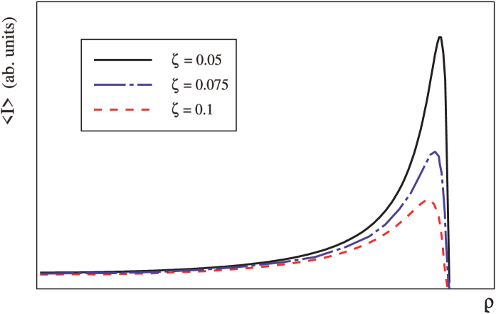
Figure 1: Instantaneous spatial distributions of the intensity in the fluctuation waveguide at different $\zeta=\frac{\left|z-z_{0}\right|}{4L_{m}}$.

The next interesting feature is that the narrow-band pulse acquires universal shape at large distances in the fluctuation waveguide. Indeed, under the assumption that in-plane distance to the observation point is such that $\rho>\tilde{c}T$, the average intensity is described by formula (34) and depends on the envelop of the incident pulse, $A(t),$ only through the normalization constant $T$. In Fig. 1, a set of curves is presented depicting the intensity distribution as a function of the in-plane distance $\varrho$ at a given time $t$ for different distances in the direction perpendicular to layers, $\zeta=\left|z-z_{0}\right|/4L_{m}$. In Fig. 2 the time dependence of the pulse intensity is shown at a certain distance $\varrho$ and three different $\zeta$. As it is seen from the graphs, during the propagation in the fluctuation waveguide the signal acquires a rather slowly decaying tail, and at large distances from the maximum of the pulse the intensity decreases in time proportionally to $t^{-2}$. The weak sensitivity of the wave packet to its initial shape is due to the fact that in randomly layered media (in distinction to free space) a point source radiates only those eigen modes that are localized in a narrow (of the size of the localization length) stripe near the source. FreiGred91 ; IEEE The (random) set of these modes is a fingerprint of each realization of random potential and is independent on the way of excitation.

1cm hang

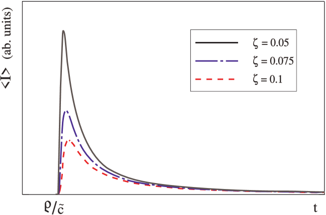
Figure 2: Time dependences of the intensity at a given in-plane distance $\varrho$ and different $\zeta=\frac{\left|z-z_{0}\right|}{4L_{m}}$.

Another peculiarity of the pulse propagation in a randomly layered medium is a sort of “anisotropy” of the time delay of the wave packet: the arrival time increases with increasing $|z-z_{0}|$ faster than it does when $\varrho$ grows. Indeed, the earliest signal arrival time at a point {${\bf\varrho,}z\}$ is of order $\frac{\sqrt{\varrho^{2}+\left(z-z_{0}\right)^{2}}}{{\tilde{c}}}$. At this moment, if $\varrho\gg L_{m}$, the spatial distribution of pulse in the fluctuation waveguide ($|z-z_{0}|<L_{m}$) given by Eq. (34) contains the exponentially small factor

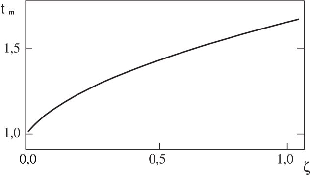
Figure 3: Arrival time of the pulse maximum, $t_{m}$ (in units $\varrho/\tilde{c}$), vs $\zeta=\frac{\left|z-z_{0}\right|}{4L_{m}}.$

$$\exp\left[-\nu(\mu)\frac{\varrho^{2}}{L_{m}|z-z_{0}|\ }\right]\ll 1\ .$$ (35)

The moment, $t_{m},$ when the signal at the point {${\bf\varrho,}z\}$ reaches its not exponentially small maximum can be roughly estimated by equating the localization exponent in (34) to unity. Ths procedure yields

$$t_{m}\sim\frac{\varrho}{\tilde{c}}\left[1-\Xi\left(\frac{z-z_{0}}{L_{m}}\right)^{2}\right]^{-1/2}$$ (36)

with some numerical coefficient $\Xi\sim 1$. Although the estimate (36) cannot claim for satisfactory accuracy, it gives a reasonable idea of the pulse delay in a stratified medium. To accurately calculate the dependence of the arraival time of the pulse maximum as a fuction of the transverse displacement $|z-z_{0}|$ one should use Eq. (34). The results of this (numerical) calculation is shown in Fig. 3.

VI Concluding remarks

To summarize, in this paper the problem of the space-time distribution of the average intensity of a narrow-band pulse which is radiated by a point source in 3D randomly layered medium has been solved by means of the generalized resonance expansion method. The pulse field is shown to be localized in the direction of stratification and channelled parallel to the layers within the fluctuation waveguide whose symmetry plane goes through the source location. The waveguide originates exclusively from the interference of random fields multiply scattered by weak fluctuations, with no regular refraction present in the medium. The typical width of the waveguide is of order of the localization length of the harmonics with largest allowable momentum along the axis of stratification. Random lamination of the medium leads to a substantial distortion of the pulse shape. Specifically, far away from the source the narrow-band pulse of any original spectral content, being locked within the fluctuation waveguide, spreads into a signal with the envelope given by the universal function (34) depicted in Figs. 1 and 2. In contrast to homogeneous media, the dependance of the arrival time of the pulse maximum on coordinates is strongly anisotropic: it increases drastically as the observation point moves in $z$-direction away from source. This delay is not due to the increase of the path length of the signal, as it is, for example, in media with regular refraction, but is caused by the multiple random scattering of the saddle-point harmonics (32).

Appendix A Calculation of the Green matrix Eq. (10)

To find the 1D Green function of Eq. (6) we express it via solutions of the appropriate Cauchy problems,

$${\cal G}(z,z_{0})={\cal W}^{-1}\left[\psi_{+}(z)\psi_{-}(z_{0})\theta(z-z_{0})+\psi_{+}(z_{0})\psi_{-}(z)\theta(z_{0}-z)\right]\ .$$ (37)

Here, the functions $\psi_{\pm}(z)$ are the linear-independent solutions of homogeneous equation (6) with boundary conditions given at either “plus” or “minus” infinity, depending on the “sign” index, ${\cal W}$ is the Wronskian of those functions, $\theta(z)$ is the Heaviside unit-step function.

In the case of real $q$, it is reasonable to represent the functions $\psi_{\pm}(z)$ as superpositions of modulated harmonic waves propagating in opposite directions of $z$-axis,

$$\psi_{\pm}(z)=\pi_{\pm}^{\Delta}(z)\exp(\pm iqz)-i\gamma_{\pm}^{\Delta}(z)\exp(\mp iqz)\ .$$ (38)

The upper index $\Delta$ indicates that the corresponding functions is related to the first Green function in Eq. (4).

Under WS conditions, (16), the “amplitudes” $\pi_{\pm}^{\Delta}(z)$ and $\gamma_{\pm}^{\Delta}(z)$ in (38) are smooth functions in comparison with the nearby standing fast exponentials. By averaging the equations for $\psi_{\pm}(z)$ over the interval of the length $2l$ intermediate between “small” and “large” lengths of Eq. (16) we arrive at a following set of dynamic equations,

$$\pm{\pi_{\pm}^{\Delta}}^{\prime}(z)+i\big{[}\eta(z)-{\Delta q^{2}}/{2q}\big{]}\pi_{\pm}^{\Delta}(z)+\zeta_{\pm}(z)\gamma_{\pm}^{\Delta}(z)=0\ ,$$ (39a)

$$\pm{\gamma_{\pm}^{\Delta}}^{\prime}(z)-i\big{[}\eta(z)-{\Delta q^{2}}/{2q}\big{]}\gamma_{\pm}^{\Delta}(z)+\zeta_{\pm}^{\ast}(z)\pi_{\pm}^{\Delta}(z)=0\ .$$ (39b)

The function $$\eta(z) \omega \omega+\Omega \zeta_{\pm}(z)$$ in (39) coincides with the analogous function from (12), with being replaced by . The functions are given by

$$\zeta_{\pm}(z)=\frac{-1}{2q}\left(\frac{\omega+\Omega}{c}\right)^{2}\int_{z-l}^{z+l}\frac{dz^{\prime}}{2l}{\rm e}^{\mp 2iqz^{\prime}}\delta\varepsilon(z^{\prime})\ .$$ (40)

Sommerfeld’s radiation conditions at $z\rightarrow\pm\infty$ are reformulated as the “initial” conditions for the smooth amplitudes,

$$\lim_{z\rightarrow\pm\infty}\pi_{\pm}^{\Delta}(z)=1\ ,\qquad\lim_{z\rightarrow\pm\infty}\gamma_{\pm}^{\Delta}(z)=0\ .$$ (41)

In a similar way the second Green function in (4) is to be represented, keeping in mind that in this case $\Delta q^{2}=0$ and $\Omega=0$.

Wronskian ${\cal W}$ in (37) within the WS limit reduces to

$${\cal W}=2iq\left[\pi_{+}^{\Delta}(z)\pi_{-}^{\Delta}(z)+\gamma_{+}^{\Delta}(z)\gamma_{-}^{\Delta}(z)\right]\ .$$ (42)

By inserting then (38) and (42) into (37) and comparing the result with Eq. (9) we obtain for the matrix elements of (10):

$${\cal G}_{1,2}(z,z_{0}|\omega+\Omega,q^{2}+\Delta q^{2})=-\frac{2\pi i}{q}A^{\Delta}(z_{0})\left[\theta_{\pm}\frac{\pi_{\pm}^{\Delta}(z)}{\pi_{\pm}^{\Delta}(z_{0})}-\theta_{\mp}\Gamma_{\pm}^{\Delta}(z_{0})\frac{\gamma_{\mp}^{\Delta}(z)}{\pi_{\mp}^{\Delta}(z_{0})}\right]\ ,$$ (43a)

$${\cal G}_{3,4}(z,z_{0}|\omega+\Omega,q^{2}+\Delta q^{2})=\ -\frac{2\pi}{q}A^{\Delta}(z_{0})\left[\theta_{\pm}\frac{\pi_{\pm}^{\Delta}(z)}{\pi_{\pm}^{\Delta}(z_{0})}\Gamma_{\mp}^{\Delta}(z_{0})+\theta_{\mp}\frac{\gamma_{\mp}^{\Delta}(z)}{\pi_{\mp}^{\Delta}(z_{0})}\right]\ .$$ (43b)

Here $$\theta_{\pm}=\theta\big{[}\pm(z-z_{0})\big{]}$$ and the rest of notations are

$$A^{\Delta}(z) = \left[1+\Gamma_{+}^{\Delta}(z)\Gamma_{-}^{\Delta}(z)\right]^{-1}\ ,$$ (44a)

$$\Gamma_{\pm}^{\Delta}(z) = \gamma_{\pm}^{\Delta}(z)/\pi_{\pm}^{\Delta}(z)\ .$$ (44b)

The upper sign indices in (43) correspond to $${\cal G}_{1} {\cal G}_{3} {\cal G}_{2} {\cal G}_{4} \Gamma_{\pm}^{\Delta}(z) \pi_{\pm}^{\Delta}(z)$$ and whereas the lower signs to and , respectively. The functions and obey the Riccati-type coupled equations resulting directly from (39),

$$\pm\frac{d\Gamma_{\pm}^{\Delta}(z)}{dz}=2i\left[\eta(z)-\frac{\Delta q^{2}}{2q}\right]\Gamma_{\pm}^{\Delta}(z)-\zeta_{\pm}^{\ast}(z)+\zeta_{\pm}(z)\left[\Gamma_{\pm}^{\Delta}(z)\right]^{2}\ ,$$ (45a)

$$\pm\frac{d}{dz}\frac{1}{\pi_{\pm}^{\Delta}(z)}=i\left[\eta(z)-\frac{\Delta q^{2}}{2q}\right]\frac{1}{\pi_{\pm}^{\Delta}(z)}+\zeta_{\pm}(z)\frac{\Gamma_{\pm}^{\Delta}(z)}{\pi_{\pm}^{\Delta}(z)}\ .$$ (45b)

The initial conditions for Eqs. (45) follow from (41).

Transition from equations (39) to (45) is motivated by the following. In the stationary and non-dissipative limiting case ($\Delta q^{2}=0$ and $\gamma=0$) the functions $\Gamma_{\pm}(z)$ represent the amplitude reflection coefficients for the harmonics $q$ incident on the 1D disordered half-spaces ($z,\pm\infty$), respectively. In the presence of arbitrary weak dissipation these functions become modulo less than unity allowing for the factor $A^{\Delta}(z)$ given by Eq. (44a) to be expanded into a series in powers of the product $\Gamma_{+}^{\Delta}\Gamma_{-}^{\Delta}$. Averaging then termwise the double series into which the product of the Green functions in (4) is expanded we arrive eventually at the expression (19).

Appendix B Analysis of the forward scattering contribution

Equation (21a) can be solved rigorously at $\alpha=0$ (see, e.g., Ref. 21, ), therefore it is not difficult to obtain an asymptotic expression for $R_{n}$ at $|\alpha|\ll 1$. With the accuracy of the first order in $\alpha^{2}$ one can find that

$$R_{n}=\beta\int_{0}^{\infty}dt\,{\rm e}^{-\beta t}\left(\frac{t}{1+t}\right)^{n}\left\{1+\alpha^{2}\left(1+2\frac{{\cal L}_{b}}{{\cal L}_{f}}\right)t\left[1+t-\frac{\beta t}{6}(3+2t)\right]\right\}\ .$$ (46)

When $|\beta|\ll 1$, the domain corresponding to $t\sim|\beta|^{-1}$ is significant in the integral (46). Therefore the contribution of the terms proportional to $\alpha^{2}$ is of the order $|{\alpha}/{\beta}|^{2}$. It follows from Eqs. (5) and (22) that

$$\left|\frac{\alpha}{\beta}\right|\lesssim\frac{\tilde{c}}{\omega{\cal L}_{b}}\ .$$ (47)

In rhs of (47) there is nothing but a small WS parameter which governs all the approximations made in the course of solution. Therefore, the terms proportional to $\alpha^{2}$ in Eq. (46) lead to the corrections that are less than the calculation accuracy, and must be omitted in (46).

To analyze the equation (21b) we present the correlation function (19), using (46) at $\alpha=0$, in the integral form,

$$K(s)=\left(\frac{2\pi}{q}\right)^{2}\frac{{\rm e}^{\beta}}{\beta}\int_{\beta}^{\infty}d\xi\,{\rm e}^{-\xi}(2\xi-\beta)\left[y_{s}(\xi)+y_{-s}(\xi)\right]\ .$$ (48)

Here $y_{s}(\xi)$ is the function related to the generating function $Y_{s}(\xi)=\sum_{n=0}^{\infty}z^{n}P_{n}(s)$ by the equality

$$y_{s}(\xi)=\frac{\xi}{\beta}Y_{s}\left(1-\frac{\xi}{\beta}\right)\ .$$ (49)

From Eq. (21b) it follows that $y_{s}(\xi)$ obeys the differential equation

$$\Bigg{[}-\frac{d}{d\xi}\xi^{2}\frac{d}{d\xi}+\xi\frac{d}{d\xi}\xi+\beta\frac{d}{d\xi}\xi\left(\frac{d}{d\xi}-1\right)+i\left(s-\frac{\Delta q^{2}}{2q}\right){\cal L}_{b}\Bigg{]} y_{s}(\xi)+\frac{1}{2}\left(\frac{\alpha}{\beta}\right)^{2}\widehat{Q}_{\beta}y_{s}(\xi)$$ (50)

$$={\cal L}_{b}\left[2+(2\xi-\beta){\rm e}^{\xi}{\rm Ei}(-\xi)+\left(\frac{\alpha}{\beta}\right)^{2}P_{\beta}(\xi)\right]\ ,$$

where

$$P_{\beta}(\xi)=\left(1+2\frac{{\cal L}_{b}}{{\cal L}_{f}}\right){\rm e}^{\beta}\int_{\beta}^{\infty}d\xi^{\prime}{\rm e}^{-\xi^{\prime}}\frac{(2\xi^{\prime}-\beta)(\xi^{\prime}-\beta)}{\xi^{\prime}+(\xi-\beta)}\left[\xi^{\prime}-(\xi^{\prime}-\beta)(2\xi^{\prime}+\beta)\right]\ ,$$ (51)

and the differential operator $\widehat{Q}_{\beta}$ has the form

$$\widehat{Q}_{\beta}= 2\left(\xi\frac{d}{d\xi}\xi\right)^{2}-\beta\left\{\xi\frac{d}{d\xi}\xi,\left\{\frac{d}{d\xi},\xi\right\}_{+}\right\}_{+}+\beta^{2}\left\{\xi\frac{d}{d\xi}\xi,\frac{d}{d\xi}\right\}_{+}$$ (54)

$$+\frac{{\cal L}_{b}}{{\cal L}_{f}}\left[4\left(\xi\frac{d}{d\xi}\xi\right)^{2}+4\beta\left(\xi\frac{d}{d\xi}\xi-\left\{\xi\frac{d}{d\xi}\xi,\frac{d}{d\xi}\xi\right\}_{+}\right)+\beta^{2}\left(1-2\frac{d}{d\xi}\xi\right)^{2}\right]\ .$$

The brackets $\{\cdots,\cdots\}_{+}$ in (54) denote an anticommutator. It is evident from (48) that the solution of Eq. (50) is of importance in the domain $\xi\lesssim 1$. In that region the estimation is valid

$$\|\widehat{Q}_{\beta}\|\sim\left|P_{\beta}(\xi)\right|\sim 1+\frac{{\cal L}_{b}}{{\cal L}_{f}}\ .$$

Thus we conclude that the terms proportional to $\widehat{Q}_{\beta}$ and $P_{\beta}(\xi)$, that contain the forward-scattering parameter ${\cal L}_{f}$, contribute negligibly, in accordance with WS parameter (47), to the solution of equation (50), just in the same way as the terms $\propto\alpha^{2}$ in (46).

References

- (1) A. Ishimaru, Wave Propagation and Scattering in Random Media, (Academic, New York, 1978).
- (2) V. D. Freilikher and S. A. Gredeskul, Prog. Opt. 30, 137 (1991).
- (3) Yu. V. Tarasov and V. D. Freilikher, Izv. Vyssh. Uchebn. Zaved. Radiofiz (USSR) 32, 1387 (1989) [SovRadiophys. (USA) 32, 1024 (1989)]; Izv. Vyssh. Uchebn. Zaved. Radiofiz (USSR) 32, 1494 (1989) [Sov Radiophys. (USA) 32, 1106 (1989)].
- (4) V. D. Freilikher and Yu. V. Tarasov, IEEE Trans. on AP 39, 197 (1991).
- (5) E. P. Wigner, Phys. Rev. 98, 145 (1955).
- (6) V. L. Berezinskii, Zh. Eksp. Teor. Fiz. (USSR) 65, 1251 (1973) [Sov. Phys.—JETP 38, 620, (1974)].
- (7) A. A. Gogolin, Phys Rep 166, 269 (1988).
- (8) A. A. Abrikosov and I. A. Ryzhkin, Adv. Phys. 27 147 (1978).
- (9) I. M. Lifshits, S. A. Gredeskul, and L. A. Pastur, Introduction to the theory of disordered systems (New York: Wiley, 1988)
- (10) N. M. Makarov and Yu. V. Tarasov, J. Phys.: Condens. Matter 10, 1523 (1998).
- (11) Yu. V. Tarasov, Waves Random Media 10, 395 (2000).
- (12) E. A. Kaner and L. V. Chebotarev, Phys. Rep. 150, 179 (1987).
- (13) E. A. Kaner and Yu. V. Tarasov, Phys. Rep. 165, 189 (1988).