Reaction, Lévy Flights, and Quenched Disorder

Abstract

We consider the $A+A\to\emptyset$ reaction, where the transport of the particles is given by Lévy flights in a quenched random potential. With a common literature model of the disorder, the random potential can only increase the rate of reaction. With a model of the disorder that obeys detailed balance, however, the rate of reaction initially increases and then decreases as a function of the disorder strength. The physical behavior obtained with this second model is in accord with that for reactive turbulent flow, indicating that Lévy flight statistics can model aspects of turbulent fluid transport.

I Introduction

Lévy flights have been used to model a variety of physical processes such as epidemic spreading Mollison (1977), self-diffusion in micelle systems Ott et al. (1990), and transport in heterogeneous rocks Klafter et al. (1990). Lévy flights are essentially a generalization of ordinary Brownian walks. The normalized step size distribution for Lévy flights in $d$ dimensions is

$$P(r)d^{d}r=\frac{fr_{0}^{f}}{S_{d}}r^{-1-f}drd\Omega$$ (1)

where $r$ is the step size, $f$ is the step index, $S_{d}=2\pi^{d/2}/(d/2-1)!$, and $r_{0}$ a lower microscopic step cutoff. In the case of $f=2$, we recover Brownian motion. However, for $f<2$, the distribution of step sizes exhibits a long-range algebraic tail that corresponds to large but infrequent steps, so called rare events. Due to these rare, large steps, the mean square step size deviation diverges, and the central limit theorem does not hold. The rare, large step events prevail and determine the long time behavior. The dynamic exponent $z$ that characterizes the mean displacement as a function of time by $\langle|r(t)|\rangle^{2}\sim({\rm const})t^{2/z}$ depends on the microscopic step index $f$ according to the relationship $z=f$, indicating anomalous enhanced diffusion, that is, superdiffusion.

It is well-known that quenched random disorder leads to sub-diffusive behavior in two-dimensional Brownian walks. Lévy flights in such random environments have attracted increasing attention recently. The interplay between the “built-in” superdiffusive behavior of the Lévy flights and the effect of the random environment generally leading to sub-diffusive behavior has been examined Fogedby (1998); Honkonen (1996, 2000). Surprisingly, an $\epsilon$ expansion shows that in the models of random potential disorder examined to date, the dynamic exponent $z$ locks onto the Lévy flight index $f$ in any dimension, regardless of the range or strength of disorder (notwithstanding some claims regarding divergence-free disorder in Honkonen (2000)).

The behavior of chemical reactions with random potential Park and Deem (1998a, b) and isotropic turbulence disorder Deem and Park (1998); le Tran et al. (1999) has been examined. Reactants diffusing according to Lévy flight statistics have also been studied in a model of branching and annihilating processes Vernon and Howard (2001). In general, potential disorder tends to slow down the diffusing reactants. Since these reactions typically become transport-limited at long times, potential disorder tends to slow down the reaction as well. It was found, however, that a small amount of potential disorder added to the turbulent fluid mixing leads to an increased rate of reaction. This phenomenon of ’superfast’ reaction occurs because the disorder traps reactants in local potential wells, which quadratically increases the local reaction rate, while the turbulence rapidly replenishes the reacting species to these regions. As the potential disorder is increased, eventually the rate of reaction decreases, due to a slowing of the transport. It is interesting to study the behavior of reactants following Lévy flight statistics in quenched random disorder. The question is: Can the Lévy statistics mimic rapid turbulent transport and so lead to superfast reaction? Furthermore, do the reactions become transport limited or reaction limited at long times?

In this paper, we analyze two different models of the disorder. A conventional literature model, which does not satisfy detailed balance, is discussed in section II. A new model that does satisfy detailed balance is discussed in section III. We study the effect of Lévy flight statistics and quenched random disorder on the simple bimolecular recombination reaction in two dimensions. We focus on the physically meaningful two-dimensional case because the effects disappear above the upper critical dimension that is near two and because other, exact methods of analysis are probably more appropriate in one dimension. Detailed results of the field theoretic renormalization are presented. We conclude this paper in section IV.

II Reaction in a Common Literature Model of Disorder

Including the normal diffusion term, the Fokker-Planck equation for Lévy flights in a quenched potential field has been modeled by Fogedby (1998); Honkonen (1996, 2000)

$$\frac{\partial G({\bf r},t)}{\partial t} = D_{2}\nabla^{2}G({\bf r},t)+D_{f}(\nabla^{2})^{f/2}G({\bf r},t)$$ (2)

$$+\nabla\cdot[G({\bf r},t)\nabla V({\bf r})]$$

where $(\nabla^{2})^{f/2}$ is interpreted as the inverse Fourier transform of $-k^{f}$, which is a spatially non-local integral operator reflecting the long-range character of the Lévy steps with microscopic step index $f$. Fourier transforms are defined as $\hat{f}({\bf k})=\int d^{d}xe^{i{\bf k}\cdot{\bf x}}f({\bf x})$. The last term on the right hand side of Eq. (2) is a drift term due to the motion of the walker in the force field. We assume a Gaussian distribution of the random potential force field, $V({\bf r})$, with correlation

$$\langle V({\bf k}_{1})V({\bf k}_{2})\rangle=\frac{\gamma}{k^{2+y}}(2\pi)^{d}\delta({\bf k}_{1}+{\bf k}_{2})$$ (3)

Note that the strength of disorder is parameterized by $\gamma$, whereas the range is parameterized by $y$.

The reaction we are considering is

$$A+A~{}{\mathrel{\mathop{\to}\limits^{\lambda}}}~{}\emptyset$$ (4)

A field theory is derived by identifying a master equation and using the coherent state mapping Lee (1994). The random potential is incorporated with the replica trick Kravtsov et al. (1985). The action within the field theory is

$$S = \int d^{d}{\bf x}\int_{0}^{t_{f}}dt\bar{a}_{i}({\bf x},t)[\partial_{t}-D_{f}(\nabla^{2})^{f/2}-D_{2}\nabla^{2}$$ (5)

$$+\delta(t)]a_{i}({\bf x},t)+\frac{\lambda}{2}\int d^{d}{\bf x}\int_{0}^{t_{f}}dt[2\bar{a}_{i}({\bf x},t)a_{i}^{2}({\bf x},t)$$

$$+\bar{a}_{i}^{2}({\bf x},t)a_{i}^{2}({\bf x},t)]-n_{0}\int d^{d}{\bf x}\bar{a}_{i}({\bf x},0)$$

$$-\frac{\gamma}{2}\int dt_{1}dt_{2}\int_{{\bf k}_{1}{\bf k}_{2}{\bf k}_{3}{\bf k}_{4}}(2\pi)^{d}\delta({\bf k}_{1}+{\bf k}_{2}+{\bf k}_{3}+{\bf k}_{4})$$

$$\times\frac{{\bf k}_{1}\cdot({\bf k}_{1}+{\bf k}_{2}){\bf k}_{3}\cdot({\bf k}_{3}+{\bf k}_{4})}{|{\bf k}_{1}+{\bf k}_{2}|^{2+y}}$$

$$\times\hat{\bar{a}}_{i}({\bf k}_{1},t_{1})\hat{a}_{i}({\bf k}_{2},t_{1})\hat{\bar{a}}_{j}({\bf k}_{3},t_{2})\hat{a}_{j}({\bf k}_{4},t_{2})$$

Summation is implied over replica indices. The notation $\int_{\bf k}$ stands for $\int d^{d}{\bf k}/(2\pi)^{d}$.

The concentration of the reactant A at time $t$, averaged over the initial conditions, is given by

$$c_{A}({\bf x},t)=\lim_{N\to 0}\langle a_{i}({\bf x},t)\rangle$$ (6)

where the average is taken with respect to $\exp(-S)$.

To apply the field theoretic renormalization procedure, the action is recast Zinn-Justin (1996) as

$$S = \int d^{d}{\bf x}\int_{0}^{t_{f}}dt\bar{a}_{i}({\bf x},t)[\partial_{t}-Z_{f}D_{fR}(\nabla^{2})^{f/2}$$ (7)

$$-\mu^{f-2}Z_{2}D_{2R}D_{fR}\nabla^{2}+\delta(t)]a_{i}({\bf x},t)$$

$$+\frac{1}{2}\mu^{f-d}Z_{\lambda}\lambda_{R}D_{fR}\int d^{d}{\bf x}\int_{0}^{t_{f}}dt[2\bar{a}_{i}({\bf x},t)a_{i}^{2}({\bf x},t)$$

$$+\bar{a}_{i}^{2}({\bf x},t)a_{i}^{2}({\bf x},t)]-\mu^{d}n_{0R}\int d^{d}{\bf x}\bar{a}_{i}({\bf x},0)$$

$$-\frac{1}{2}\mu^{\epsilon}Z_{\gamma}\gamma_{R}D_{fR}^{2}\int dt_{1}dt_{2}\int_{{\bf k}_{1}{\bf k}_{2}{\bf k}_{3}{\bf k}_{4}}(2\pi)^{d}$$

$$\times\delta({\bf k}_{1}+{\bf k}_{2}+{\bf k}_{3}+{\bf k}_{4})\frac{{\bf k}_{1}\cdot({\bf k}_{1}+{\bf k}_{2}){\bf k}_{3}\cdot({\bf k}_{3}+{\bf k}_{4})}{|{\bf k}_{1}+{\bf k}_{2}|^{2+y}}$$

$$\times\hat{\bar{a}}_{i}({\bf k}_{1},t_{1})\hat{a}_{i}({\bf k}_{2},t_{1})\hat{\bar{a}}_{j}({\bf k}_{3},t_{2})\hat{a}_{j}({\bf k}_{4},t_{2})$$

where the renormalization constants $Z_{f},Z_{2},Z_{\lambda}$, and $Z_{\gamma}$ have been introduced to absorb the UV divergences of the model. The parameters, $D_{fR},D_{2R},\lambda_{R},$ and $\gamma_{R}$ are the dimensionless expansion parameters of the model. Since the Lévy flight term, $D_{fR}(\nabla^{2})^{f/2}$, is the most important term, it is chosen as the dimensionless free term, i.e. the propagator is $[\partial_{t}-D_{fR}(\nabla^{2})^{f/2}]^{-1}$. Note, we are not allowed to treat the regular diffusion term as free term, as this violates the physics of the scaling and leads to a diverging renormalized $D_{f}$. Now, the critical dimension following from standard power counting of $\gamma_{R}$ is $d_{c}=2f+y-2$, and we introduce for an $\epsilon$ expansion $\epsilon=d_{c}-d$. The scale-setting wavenumber parameter is denoted by $\mu$, and we assign the dimensions to the rest of the terms accordingly.

The connections between the renormalized and unrenormalized parameters are

$$Z_{f}D_{fR} = D_{f}$$

$$\mu^{f-2}Z_{2}D_{2R}D_{fR} = D_{2}$$

$$\mu^{f-d}Z_{\lambda}\lambda_{R}D_{fR} = \lambda$$

$$\mu^{d}n_{0R} = n_{0}$$

$$\mu^{\epsilon}Z_{\gamma}\gamma_{R}D_{fR}^{2} = \gamma$$ (8)

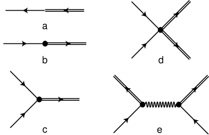
Figure 1: (a) Diagram representing the propagator. The arrow points in the direction of increasing time, and double lines represent the bar fields. (b) Normal diffusion vertex $D_{2}$. (c), (d) Reaction vertices $\lambda$. (e) Disorder vertex $\gamma$.

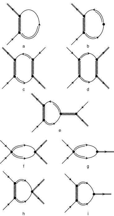
Figure 2: One-loop diagrams: (a) self-energy diagram contributing to $D_{f}$; (b) self-energy diagram contributing to $D_{2}$; (c), (d), and (e) vertex diagrams contributing to $\gamma$; (f), (g), (h), and (i) vertex diagrams contributing to $\lambda$.

To one-loop order, self-energy diagrams and vertex diagrams are summarized in Fig. 1 and Fig. 2. We may be tempted to use the momentum-shell renormalization procedure here. However, due to the difficulty of regularizing this action, the first self-energy diagram would incorrectly contribute to $D_{2R}$ by the momentum-shell renormalization, rather than to $D_{fR}$ by the field theoretic renormalization that is consistent with perturbation theory. In the evaluation of the diagram in Fig. 2a, it is important to treat the external momentum exactly. If a series expansion in the external momentum is performed on the integrand, rather than on the result of the integral, an incorrect contribution to $Z_{2}$ arises. Interestingly, when the diagram in Fig. 2a is evaluated, only a finite contribution to $Z_{f}$ results. Complete calculation shows

$$Z_{f} = 1$$

$$Z_{2} = 1-\frac{(2f-3)\gamma}{4\pi\epsilon}$$

$$Z_{\lambda} = 1-\frac{\gamma_{R}}{2\pi\epsilon}+\frac{\lambda_{R}}{4\pi(f-d)}$$

$$Z_{\gamma} = 1+\frac{\gamma_{R}}{2\pi\epsilon}$$ (9)

where a double pole expansion, $1/\epsilon$ and $1/(f-d)$, is used in the calculation of $Z_{\lambda}$. The use of the double pole expansion in two dimensions means we consider $f$ just slightly smaller than $2$ and $y$ small. As usual, the $\beta$ functions defined by

$$\beta_{D_{2R}} = \mu\frac{\partial}{\partial\mu}D_{2R}$$

$$\beta_{\lambda_{R}} = \mu\frac{\partial}{\partial\mu}\lambda_{R}$$

$$\beta_{\gamma_{R}} = \mu\frac{\partial}{\partial\mu}\gamma_{R}$$ (10)

give the flow equations in two dimensions as

$$\frac{dD_{2R}}{dl} = -\beta_{D_{2R}}=(f-2)D_{2R}+\frac{(2f-3)\gamma_{R}D_{2R}}{4\pi}$$

$$\frac{d\lambda_{R}}{dl} = -\beta_{\lambda_{R}}=(f-2)\lambda_{R}+\frac{\gamma_{R}\lambda_{R}}{2\pi}-\frac{\lambda_{R}^{2}}{4\pi}$$

$$\frac{d\gamma_{R}}{dl} = -\beta_{\gamma_{R}}=\epsilon\gamma_{R}-\frac{\gamma_{R}^{2}}{2\pi}$$ (11)

where we use the relation $\mu=\Lambda/e^{l}$, and $\Lambda$ is a microscopic cutoff. Since $Z_{f}=1$, the reaction and disorder terms do not affect the dynamic exponent, and $z=f$. We determine the long-time decay from the flow equation via matching to short-time perturbation theory. The flow equations are integrated to a short time such that

$$t(l^{*})=t\exp[-\int_{0}^{l^{*}}z(l)dl]=t_{0}$$ (12)

At short times, we find the mean displacement of an unreactive particle from $\langle|r(t(l^{*}),l^{*})|\rangle^{f}=4D_{f}t(l^{*})$, and the concentration of reactants from $c_{A}(t(l^{*}),l^{*})=[(n_{0R}(l^{*})\Lambda^{d})^{-1}+D_{f}\lambda_{R}(l^{*})\Lambda^{f-2}t(l^{*})]^{-1}$. The long-time asymptotic values are given by scaling: $\langle|r(t)|\rangle^{f}=e^{fl^{*}}\langle|r(t(l^{*}),l^{*})|\rangle^{f}$, and $c_{A}(t)=e^{-2l^{*}}c_{A}(t(l^{*}),l^{*})$.

We first investigate the behavior of $D_{2R}$. As we will see below, the fixed point for $\gamma_{R}$ is $\max(0,2\pi\epsilon)$. Using this result, we see that $D_{2R}$ flows exponentially to zero as long as $y<4(2-f)$, when $f$ is near 2. Likely, a higher loop calculation would extend the region in which $D_{2R}$ flows to zero. Thus, at least within the region in which our flow equations apply, $D_{2R}$ always flows to 0 in the presence of Lévy flights. It is, therefore, unnecessary to introduce such a normal diffusion term in the model.

Figure 3: Different regions predicted by the flow equations for the Lévy flight system with disorder model I in two dimensions. The flow equation are accurate for small $y$ and $f$ slightly less than 2. The flow equations do not apply in region IV.

For $\epsilon<0$, i.e. in region I of Fig. 3, there is only a set of trivial stable fixed points, $\gamma_{R}^{*}=0$ and $\lambda_{R}^{*}=0$, for the system. The matching procedure gives the normal concentration decay as

$$c_{A}(t)\sim\frac{1}{\lambda t}$$ (13)

In the region of $\epsilon>0$, $\gamma_{R}^{*}=2\pi\epsilon$ is the nontrivial fixed point. But depending on the value of $\delta=3f+y-6$, the matching procedure yields different results. For $\delta<0$, i.e. in region II of Fig. 3, there is no non-trivial fixed point for $\lambda_{R}$. The corresponding asymptotic concentration decay is a little faster than that in region I:

$$c_{A}(t)\sim\frac{1}{t_{0}}\left(\frac{1}{\lambda}+\frac{1}{4\pi|\delta|D_{f}\Lambda^{f-2}}\right)\left(\frac{t}{t_{0}}\right)^{-\frac{2-|\delta|}{f}}$$ (14)

For $\delta>0$, i.e. in region III of Fig. 3, $\lambda_{R}^{*}=4\pi\delta$ is the fixed point. The asymptotic concentration decay is the fastest:

$$c_{A}(t)\sim\frac{1}{4\pi\delta D_{f}\Lambda^{f-2}t_{0}}\left(\frac{t}{t_{0}}\right)^{-\frac{2}{f}}$$ (15)

The relationship between the concentration decay exponent, $\alpha$, and disorder range, $y$, at a fixed value of $f$ is plotted in Fig 4. Note that the strength of the disorder has no effect whatsoever on the concentration decay.

Figure 4: Decay exponent for the $A+A\to\emptyset$ reaction in the Lévy flight system with disorder model I in two dimensions: $c_{A}(t)\sim({\rm const})t^{-\alpha}$.

The reader will note that the disorder can never slow down the reaction in this model. This is quite an unexpected result, as these reactions are expected to become transport-limited at long times, and disorder should slow down the transport. Model I, Eq. (2), is somewhat unphysical in that this cannot happen due to the lack of disorder contribution to $Z_{f}$.

III Reaction in a Model of Disorder that Obeys Detailed Balance

Although Eq. (2) is often used in the literature, it does not guarantee a long-time Boltzmann distribution for $G({\bf r},t)$. That is, this form of the disorder does not satisfy detailed balance. A more natural form of the Fokker-Planck equation for Lévy flights in random disorder is

$$\frac{\partial G({\bf r},t)}{\partial t}=\nabla^{f-1}\cdot[D_{f}\nabla G({\bf r},t)+G({\bf r},t)\nabla V({\bf r})]$$ (16)

where $\nabla^{f-1}$ is the inverse Fourier transform of $-ik^{f-2}{\bf k}$. Equation (16) can be interpreted as a modification of the continuity equation to take into account the long-range transport induced by the Lévy flights; it is derived in the appendix. With the same form of the correlation function for the potential, Eq. (3), we have

$$S = \int d^{d}{\bf x}\int_{0}^{t_{f}}dt\bar{a}_{i}({\bf x},t)[\partial_{t}-D_{f}(\nabla^{2})^{f/2}+\delta(t)]a_{i}({\bf x},t)$$ (17)

$$+\frac{\lambda}{2}\int d^{d}{\bf x}\int_{0}^{t_{f}}dt[2\bar{a}_{i}({\bf x},t)a_{i}^{2}({\bf x},t)+\bar{a}_{i}^{2}({\bf x},t)a_{i}^{2}({\bf x},t)]$$

$$-n_{0}\int d^{d}{\bf x}\bar{a}_{i}({\bf x},0)$$

$$-\frac{\gamma}{2}\int dt_{1}dt_{2}\int_{{\bf k}_{1}{\bf k}_{2}{\bf k}_{3}{\bf k}_{4}}(2\pi)^{d}\delta({\bf k}_{1}+{\bf k}_{2}+{\bf k}_{3}+{\bf k}_{4})$$

$$\times\frac{k_{1}^{f-2}k_{3}^{f-2}{\bf k}_{1}\cdot({\bf k}_{1}+{\bf k}_{2}){\bf k}_{3}\cdot({\bf k}_{3}+{\bf k}_{4})}{|{\bf k}_{1}+{\bf k}_{2}|^{2+y}}$$

$$\times\hat{\bar{a}}_{i}({\bf k}_{1},t_{1})\hat{a}_{i}({\bf k}_{2},t_{1})\hat{\bar{a}}_{j}({\bf k}_{3},t_{2})\hat{a}_{j}({\bf k}_{4},t_{2})$$

Again, to apply the field theoretic renormalization procedure, the action is recast as

$$S = \int d^{d}{\bf x}\int_{0}^{t_{f}}dt\bar{a}_{i}({\bf x},t)[\partial_{t}-Z_{f}D_{fR}(\nabla^{2})^{f/2}$$

$$+\delta(t)]a_{i}({\bf x},t)+\frac{1}{2}\mu^{f-d}Z_{\lambda}\lambda_{R}D_{fR}\int d^{d}{\bf x}\int_{0}^{t_{f}}dt$$

$$\times[2\bar{a}_{i}({\bf x},t)a^{2}_{i}({\bf x},t)+\bar{a}_{i}^{2}({\bf x},t)a_{i}^{2}({\bf x},t)]$$

$$-\mu^{d}n_{0R}\int d^{d}{\bf x}\bar{a}_{i}({\bf x},0)-\frac{1}{2}\mu^{\epsilon}Z_{\gamma}\gamma_{R}D_{fR}^{2}\int dt_{1}dt_{2}$$

$$\times\int_{{\bf k}_{1}{\bf k}_{2}{\bf k}_{3}{\bf k}_{4}}(2\pi)^{d}\delta({\bf k}_{1}+{\bf k}_{2}+{\bf k}_{3}+{\bf k}_{4})$$

$$\times\frac{k_{1}^{f-2}k_{3}^{f-2}{\bf k}_{1}\cdot({\bf k}_{1}+{\bf k}_{2}){\bf k}_{3}\cdot({\bf k}_{3}+{\bf k}_{4})}{|{\bf k}_{1}+{\bf k}_{2}|^{2+y}}$$

$$\times\hat{\bar{a}}_{i}({\bf k}_{1},t_{1})\hat{a}_{i}({\bf k}_{2},t_{1})\hat{\bar{a}}_{j}({\bf k}_{3},t_{2})\hat{a}_{j}({\bf k}_{4},t_{2})$$

where, $d_{c}=2+y$, $\epsilon=d_{c}-d$, and the rest of the parameters are the same as in action I.

The connections between the renormalized and unrenormalized parameters are

$$Z_{f}D_{fR} = D_{f}$$

$$\mu^{f-d}Z_{\lambda}\lambda_{R}D_{fR} = \lambda$$

$$\mu^{d}n_{0R} = n_{0}$$

$$\mu^{\epsilon}Z_{\gamma}\gamma_{R}D_{fR}^{2} = \gamma$$ (19)

The diagrams are the same as those in Figs. 1 and 2, except that the diagrams from normal diffusion, Figs.  1b and 2b, are not present. A one-loop diagrammatic calculation gives

$$Z_{f} = 1+\frac{\gamma_{R}}{4\pi\epsilon}$$

$$Z_{\lambda} = 1-\frac{\gamma_{R}}{2\pi\epsilon}+\frac{\lambda_{R}}{4\pi(f-d)}$$

$$Z_{\gamma} = 1+\frac{\gamma_{R}}{2\pi\epsilon}$$ (20)

where a double-pole expansion of $1/\epsilon$ and $1/(f-d)$ is used in the calculation of $Z_{\lambda}$.

The dynamic exponent is given by

$$z=f-\mu\frac{\partial}{\partial\mu}\ln Z_{f}=f+\frac{\gamma_{R}}{4\pi}$$ (21)

This suggests that the Lévy flights are significantly slowed by the presence of the new random disorder term. That is, when detailed balance is obeyed, the disorder affects the dynamical exponent.

The $\beta$ functions give us the flow equations from $Z_{i}$ in two dimensions as

$$\frac{d\lambda_{R}}{dl} = -\beta_{\lambda_{R}}=(f-2)\lambda_{R}+\frac{3\gamma_{R}\lambda_{R}}{4\pi}-\frac{\lambda_{R}^{2}}{4\pi}$$

$$\frac{d\gamma_{R}}{dl} = -\beta_{\gamma_{R}}=\epsilon\gamma_{R}$$ (22)

This action is well-behaved, and there is no regularization difficulty. And indeed, both momentum-shell renormalization and field-theoretic renormalization yield identical flow equations to one-loop order. From the flow equations, for $\epsilon>0$, $\gamma_{R}$ flows to $\infty$, indicating that the disorder dominates over the Lévy flights. For $\epsilon<0$, $\gamma_{R}$ flows to $0$, indicating transport of Lévy flights dominates over the disorder. This same behavior, that the disorder must be adjusted to be compatible with the transport, was found in the turbulent reactive flow problem le Tran et al. (1999). An interesting system arises when those two effects are competitive, and so we require $\epsilon=0$, i.e. $y=0$. Under this constraint, $\gamma_{R}=\gamma/D_{f}^{2}$ does not flow. Very likely, this result holds to all orders. Further analysis of the flow equation for $\lambda_{R}$ indicates two regimes. For $\gamma/D_{f}^{2}>4(2-f)\pi/3$, or strong disorder, $\lambda_{R}$ has a stable nontrivial fixed point, given by

$$\lambda_{R}^{*}=4\pi(f-2)+\frac{3\gamma}{D_{f}^{2}}=\lambda^{*}\Lambda^{2-f}/D_{f}$$ (23)

Following the matching procedure, we have

$$c_{A}(t)\sim\frac{1}{\lambda^{*}t}\left(\frac{t}{t_{0}}\right)^{-\frac{2}{f+\gamma/(4\pi D_{f}^{2})}+1}$$ (24)

However, for $\gamma/D_{f}^{2}<4(2-f)\pi/3$, or weak disorder, there is no nontrivial fixed point for $\lambda_{R}$, and we have

$$c_{A}(t) \sim \left(\frac{1}{\lambda}+\frac{1}{[4\pi(2-f)-3\gamma/D_{f}^{2}]\Lambda^{f-2}D_{f}}\right)$$ (25)

$$\times\frac{1}{t}\left(\frac{t}{t_{0}}\right)^{-\frac{\gamma/(2\pi D_{f}^{2})}{f+\gamma/(4\pi D_{f}^{2})}}$$

For the special case of $\gamma/D_{f}^{2}=4(2-f)\pi/3$, $\lambda_{R}$ decays marginally, and we have a logarithmic correction to the decay:

$$c_{A}(t)\sim\frac{3\ln(t/t_{0})}{8\pi D_{f}\Lambda^{f-2}(1+f)t}\left(\frac{t}{t_{0}}\right)^{-\frac{2-f}{1+f}}$$ (26)

Figure 5: Decay exponent for the $A+A\to\emptyset$ reaction in the Lévy flight system that obeys detailed balance in two dimensions: $c_{A}(t)\sim({\rm const})t^{-\alpha}$. The figure is shown for $f=1.9$. The reaction is transport limited on the solid curve and reaction limited on the dashed curve. Note that the region $\alpha>1$ corresponds to ’superfast’ reaction.

In the present case, unlike with the action of section II, the range and strength of disorder affect the decay exponent significantly. The relationship between the decay exponent and $\gamma$ is plotted in Fig. 5. We see that a small amount of potential disorder leads to an increased rate of reaction in the Lévy flights. But as the potential disorder increases further, the rate of reaction eventually decreases. This figure is very much similar to the one that showed up in the study of reactive turbulent flow Deem and Park (1998). In fact, if the Lévy flight parameters are related to the turbulence parameters Deem and Park (1998) as $f=2-g^{*}_{\sigma}$ and $\gamma=4\pi D_{f}^{2}g^{*}_{\gamma}$, these two models predict exactly the same concentration decays. As suggested in Deem and Park (1998), in order for the reaction to occur, multiple reactants must be trapped in regions of low potential energy. After the trapped reactants are depleted, new reactants must be replenished by rapid transport to continue the reaction. Certain combinations of fast transport, $f<2$, and disorder, $\gamma$, lead to ’superfast’ reaction, $\alpha>1$, as shown in Fig. 5. Interestingly, this result means that the inhomogeneous system can have a faster reaction rate than the homogeneous, well-mixed system.

IV Conclusion

We have analyzed the $A+A\to\emptyset$ reaction in two dimensional Lévy flight systems using two models of random disorder. For a common model in the literature, the dynamic exponent always locks to the microscopic step index $f$, and the reaction decay exponent varies between 1 and $2/f$. This surprisingly unphysical result that the disorder cannot slow down the reaction is due to the fact that this model does not satisfy detailed balance. For a model that does satisfy detailed balance, on the other hand, the disorder can and does modify the transport properties of the system. When the disorder is adjusted to be compatible with the Lévy flight statistics, the reaction decay exponent first rises above unity and then drops to zero as the strength of disorder is increased. These results are identical to those from reactive turbulent flow, and this harmony suggests that Lévy flights, properly interpreted, can be a viable model of turbulent fluid transport.

Appendix

In this appendix, we derive Eq. (16) from a master equation. Particle transport by Lévy flight statistics can be modeled by hopping dynamics of particles in space. The hopping rate in the absence of an external potential is simply proportional to Eq. (1). In the presence of an external potential, we modify this rate in a way that satisfies detailed balance Pham and Deem (1998):

$$\alpha({\bf r}_{\rm o}\to{\bf r}_{\rm n})=(D_{f}/r_{0}^{f})P({\bf r}_{\rm n}-{\bf r}_{\rm o})e^{-\beta[V({\bf r}_{\rm n})-V({\bf r}_{\rm o})]/2}$$ (27)

where $\alpha({\bf r}_{\rm o}\to{\bf r}_{\rm n})$ is the rate at which particles hop from ${\bf r}_{\rm o}$ to ${\bf r}_{\rm n}$. The master equation for the Green’s function of this process is

$$\frac{\partial G({\bf r})}{\partial t} = \int d^{d}{\bf x}~{}\alpha({\bf r}-{\bf x}\to{\bf r})G({\bf r}-{\bf x})$$ (28)

$$-\int d^{d}{\bf x}~{}\alpha({\bf r}\to{\bf r}+{\bf x})G({\bf r})$$

We now expand this master equation to first order in $\beta$, i.e. we look for a Fokker-Planck equation that is linear in the potential. Noting that $\hat{P}({\bf k})=1-r_{0}^{f}k^{f}$, we find

$$\frac{\partial\hat{G}({\bf k})}{\partial t} = -D_{f}k^{f}\hat{G}({\bf k})-\frac{\beta D_{f}}{2}\int_{\bf h}\hat{G}({\bf k}-{\bf h})\hat{V}({\bf h})$$ (29)

$$\times[k^{f}+h^{f}-|{\bf k}-{\bf h}|^{f}]+O({\beta^{2}})$$

In real space, we would write this equation as

$$\frac{\partial G({\bf r})}{\partial t}= D_{f}(\nabla^{2})^{f/2}G+\frac{\beta D_{f}}{2}\bigg{[}(\nabla^{2})^{f/2}(GV)$$ (30)

$$+G(\nabla^{2})^{f/2}V-V(\nabla^{2})^{f/2}G\bigg{]}$$

Since we are interested in how the long-wavelength features of the potential affect the dynamics, i.e. we take into account only the small wavevector contributions in Eq. (3), we make an expansion of Eq. (29) for small $h$. We find $(k^{f}+h^{f}-|{\bf k}-{\bf h}|^{f})/2\sim fk^{f-2}{\bf k}\cdot{\bf h}/2$ for $1<f\leq 2$. Realizing that the Green’s function should relax to the Boltzmann distribution at long times, and that $D_{f}$ and $\beta$ may be renormalized a finite amount by a variety of irrelevant operators, we conclude that the proper long-wavelength theory should be

$$\frac{\partial\hat{G}({\bf k})}{\partial t} = -D_{f}k^{f}\hat{G}({\bf k})$$ (31)

$$-\beta D_{f}\int_{\bf h}\hat{G}({\bf k}-{\bf h})\hat{V}({\bf h})k^{f-2}{\bf k}\cdot{\bf h}$$

which is exactly Eq. (16) with units of $\beta$ inserted.

References

• Mollison (1977) D. Mollison, J. R. Stat. Soc. B 39, 283 (1977).
• Ott et al. (1990) A. Ott, J. P. Bouchaud, D. Langevin, and W. Urbach, Phys. Rev. Lett. 65, 2201 (1990).
• Klafter et al. (1990) J. Klafter, A. Blumen, G. Zumofen, and M. F. Shlesinger, Physica A 168, 637 (1990).
• Fogedby (1998) H. C. Fogedby, Phys. Rev. E 58, 1690 (1998).
• Honkonen (1996) J. Honkonen, Phys. Rev. E 53, 327 (1996).
• Honkonen (2000) J. Honkonen, Phys. Rev. E 62, 7811 (2000).
• Park and Deem (1998a) J.-M. Park and M. W. Deem, Phys. Rev. E 57, 2681 (1998a).
• Park and Deem (1998b) J.-M. Park and M. W. Deem, Phys. Rev. E 57, 3618 (1998b).
• Deem and Park (1998) M. W. Deem and J.-M. Park, Phys. Rev. E 58, 3223 (1998).
• le Tran et al. (1999) N. le Tran, J.-M. Park, and M. W. Deem, J. Phys. A: Math. Gen. 32, 1407 (1999).
• Vernon and Howard (2001) D. Vernon and M. Howard, Phys. Rev. E 63, 041116 (2001).
• Lee (1994) B. P. Lee, J. Phys. A: Math. Gen. 27, 2633 (1994).
• Kravtsov et al. (1985) V. E. Kravtsov, I. V. Lerner, and V. I. Yudson, J. Phys. A: Math. Gen. 18, L703 (1985).
• Zinn-Justin (1996) J. Zinn-Justin, Quantum Field Theory and Critical Phenomena (Clarendon Press, Oxford, 1996), 3rd ed.
• Pham and Deem (1998) V. Pham and M. W. Deem, J. Phys. A: Math. Gen. 31, 7235 (1998).