Conductance scaling at the band center of wide wires with pure non–diagonal disorder

Abstract

Kubo formula is used to get the scaling behavior of the static conductance distribution of wide wires showing pure non–diagonal disorder. Following recent works that point to unusual phenomena in some circumstances, scaling at the band center of wires of odd widths has been numerically investigated. While the mean conductance shows a decrease that is only proportional to the inverse square root of the wire length, the median of the distribution exponentially decreases as a function of the square root of the length. Actually, the whole distribution decays as the inverse square root of the length except close to $G=0$ where the distribution accumulates the weight lost at larger conductances. It accurately follows the theoretical prediction once the free parameter is correctly fitted. Moreover, when the number of channels equals the wire length but contacts are kept finite, the conductance distribution is still described by the previous model. It is shown that the common origin of this behavior is a simple Gaussian statistics followed by the logarithm of the $E=0$ wavefunction weight ratio of a system showing chiral symmetry. A finite value of the two–dimensional mean conductance is obtained in the infinite size limit. Both conductance and the wavefunction statistics distributions are given in this limit. This results are consistent with the critical character of the $E=0$ wavefunction predicted in the literature.

I Introduction

The existence of peculiar properties that differentiate pure non–diagonal disorder models from disorder models including diagonal disorder has a long history. Probably, the first contribution along this line corresponds to Dyson’s work on a one–dimensional phonon model published in 1953dyson . The existence of a divergent density of states at the band center of such disordered systems implying a divergent localization length was pointed in later works1d_a ; 1d_b . Since then many works on this subject have been published (a representative list can be found in Ref.(mudry0, )). The existence of some kind of delocalization transition at the band center of such models certainly disturbs the widely accepted statement saying that the specific form of disorder does not matter in single parameter scaling theoryeconomou .

A bipartite lattice is a lattice that can be divided into two sublattices such that the Hamiltonian changes sign under a transformation that changes the sign of the wavefunction on one sublattice. When pure non–diagonal disorder is considered on a bipartite lattice, the electron-hole symmetry of the spectrum is not destroyed by disorder. This property has important consequences as, for example, the existence of an eigenstate at $E=0$ for any disorder realization of a system constituted by an odd number of sites (the spectrum shows $\pm E_{\alpha}$ pairs plus a state at $E=0$). Recently, several works pointing to the exotic behavior of transport properties of quantum wires showing chiral symmetry have been publishedmudry0 ; mudry . For example, scaling of the conductance strongly depends on the parity of the number of channels along the wire. Also, related activity in field theory has produced several models demonstrating a delocalization transition in the vicinity of the zero energy statecampos .

In this paper, the scaling properties of the simplest disorder model preserving chiral symmetry have been carefully analyzed at the band center of quantum wires. Numerical simulation has been used to get the whole distribution of conductances. While the mean value of the conductance decays algebraically for wires of odd width, an alternative measure of the central value of distributions -the median- shows an exponential decay. Actually, the larger part of the conductance measurements has an exponentially small value for large wires. Therefore, although the conductance distribution is certainly peculiar at the band center, I would still use the term exponential localization when referring to the scaling behavior of the conductance of long wires. Results change when width and length of the wire coincide. In this case, the numerical simulation presented in this paper uses a dot geometry point of view keeping the size of the contacts finite while dot area scaling proceeds. The conductance distribution converges to a well defined limit that is compatible with the predicted critical behavior of the state at the band center. It is shown that the analytic form used to fit conductance distributions comes from a new underlying wavefunction statistics describing the distribution of weight ratios of the $E=0$ wavefunction.

The format of the paper is as follows. Section II defines a quite simple chain model that allows some analytical results and an unbound numerical simulation. Section III gives a more general disorder model on finite rectangular clusters of the square lattice. The way in which the conductance is calculated is presented in Section IV. Numerical results are given in Section V, first for wide disordered wires and, second, for square clusters. The last Section of the paper compiles the main conclusions reached by this numerical study of conductance scaling.

II Toy model

Let me begin with a detailed description of the scaling properties of the conductance of a chain showing pure non–diagonal disorder. In this case, sign changes of the hopping parameters do not matter and changes in their absolute value should be considered. One case that allows some analytic results consists of a chain with hopping parameters that randomly take values of $1$ and $\sqrt{2}$ with equal probability. Starting from the selfenergy of an ideal chain at its band center $\Sigma_{0}=-i$, successive selfenergies can be obtained through the disordered part of the chain by means of the usual iterative sequence (see, for example, Eqs. (7)-(10) in Ref.(1d_b, )):

$$\Sigma_{n+1}=-{{t_{n}}^{2}\over\Sigma_{n}}\qquad,$$ (1)

where ${t_{n}}^{2}$ takes values 1 or 2 with equal probability. Since selfenergy remains purely imaginary, a more convenient form is possible:

$$-\Sigma_{n+1}/i={{t_{n}}^{2}\over(-\Sigma_{n}/i)}\qquad.$$ (2)

The conductance $G$ of a sample is obtained from the selfenergy at the end of the disordered chain part $\Sigma_{N}/i$:

$$G={{4(-\Sigma_{0}/i)(-\Sigma_{N}/i)}\over[1+(-\Sigma_{0}/i)(-\Sigma_{N}/i)]^{2}}={{4(-\Sigma_{N}/i)}\over[1+(-\Sigma_{N}/i)]^{2}}\qquad.$$ (3)

Eq. (3) shows that the conductance varies between 0 and 1 as it corresponds to a one–channel system. Actually, the conductance takes the value 1 only if $-\Sigma_{N}/i=-\Sigma_{0}/i=1$. Repeated use of Eq.(2) shows that the form in which the random hopping elements appear in the selfenergy expression is:

$$\frac{{t_{0}}^{2}{t_{2}}^{2}{t_{4}}^{2}...}{{t_{1}}^{2}{t_{3}}^{2}{t_{5}}^{2}...}\qquad.$$ (4)

Therefore, a perfect transmission through the chain is obtained when the number of normal (hopping equal to 1) and strong (hopping equal to $\sqrt{2}$) bonds of the numerator coincides with the corresponding numbers of the denominator. Solving this simple combinatorial problem, one gets a probability

$$p(G=1)={1\over 2^{N}}\sum_{n=0}^{N/2}\>\bigg{[}{(N/2)!\over{(N/2-n)!n!}}\bigg{]}^{2}$$ (5)

for the peak of the probability distribution of the conductance at $G=1$curiosidad . Notice that the distribution is a sum of delta functions since the hopping takes just two different values; for example, the peak below the one at $G=1$ appears at $G=8/9$ and corresponds to $-\Sigma_{N}/i=2$ or $-\Sigma_{N}/i=1/2$ (one extra strong bond either in the numerator or the denominator). An asymptotic expansion for large enough chain lengths can be found for the sum in (5):

$$p(G=1)\sim\sqrt{2\over{\pi N}}\qquad.$$ (6)

The scaling behavior of this peak is enough to explain an inverse square root law for the mean value of $G$ given that other peaks of the distribution decay in a similar or faster way with the size of the chain. This is an interesting behavior since it perfectly coincides with scaling predictions for wide wires of odd number of transversal modesmudry .

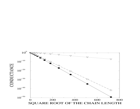
Figure 2: Length scaling for the model of Fig. 1 when the conductance distribution is described by an alternative central value such as the average value of the logarithm (filled circles), the median (empty circles) or the conductance value at which the integral of the distribution reaches a value of 0.9 (down triangles). All of them are fitted in the whole range of chain lengths by an exponential law decaying as a function of the square root of the sample length.

Numerical simulations can be done as precise as necessary for this simple model. This fact allows a detailed comparison with theoretical predictions. Fig. 1 shows the scaling of the conductance as described by its mean value. Root mean square deviation is about some tenths of the conductance unit. In any case, the average conductance at large sizes ($N>1000$) shows a power law scaling with the distance that is compatible with the inverse square root law given by Eq.(6). According with this result, a disordered chain with pure non–diagonal disorder shows non–standard scaling at the band center. Nevertheless, alternative measures of the central value of the distribution restore to some way the usual exponential decay of one–dimensional conductances, even in the presence of chiral symmetry. For example, the geometric mean of the same conductance distributions shows a much more pronounced decrease with length (see Fig. 2) although the corresponding standard deviation is of the same order as the mean making doubtful its statistical relevance. But there are other alternatives which do give a good description of the overall scaling of the distribution. Both the median or any definition based on the value of the integral of the distribution between 0 and an arbitrary upper limit $G_{\rm max}$ flow to exponentially small values. The physical meaning is clear in this case: half or more of the measures are exponentially small at large chain lengths. Actually, the precise scaling law for these central value alternatives is:

$$G_{0}\sim\exp\Big{(}-\sqrt{L/\xi}\Big{)}\qquad,$$ (7)

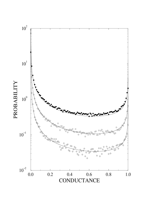
Figure 4: Length scaling of the probability distribution of conductances of a nine channel wire. Filled circles, empty circles and diamonds give histograms for the statistics of $10^{5}$ samples of lengths 100, 1000 and 10000, respectively. Continuous lines give results obtained from Eq. (10). Conductance unit is ${e^{2}}/h$.

where $\xi$ gives a measure of the exponential localization length. Fig. 2 shows that fits according to this law are excellent over the whole length range. The ultimate reason for such statistically disappointing results is simply the unusual size scaling of the distribution. While the major part of the distribution below $G=1$ decays in an algebraic form, the weight of the distribution accumulates in an exponentially small region near $G=0$ (Fig. 4 in Section V illustrates graphically this behavior). In this way, the upper part of the distribution dominates the scaling behavior of mean, root mean square deviation, etc., while accumulation at $G=0$ gives the behavior of central value definitions based on the integral of the distribution. In my opinion, these last definitions are better suited for characterizing the whole distribution than standard averages. Ultimately, one should look at the precise experimental protocol followed to get a value of the conductance before making predictions about the result of the measurements.

III Non–diagonal disorder model

The lattice Hamiltonian describing random hopping on a $L\times M$ cluster of the square lattice is :

$$\hat{H}={\sum_{<ll^{\prime}>}t_{ll^{\prime}}\hat{c}_{l}^{{\dagger}}\hat{c}_{l^{\prime}}}\qquad,$$ (8)

where $\hat{c}_{l}^{{\dagger}}$ creates an electron on site $l$, $l$ and $l^{\prime}$ are nearest–neighbor sites, and $t_{ll^{\prime}}$ is the hopping energy from site $l$ to $l^{\prime}$. It takes values 1 and -1 with equal probability. Let me refer to this model as the Random Hopping Sign (RHS) model. Obviously, the square lattice can be divided into two sublattices such that atoms belonging to one of them hop only to sites belonging to the other sublattice when described by Hamiltonian (8). Therefore, this Hamiltonian changes sign under a transformation that changes the sign of the electron operators on one sublattice. Consequently, the spectrum is symmetric relative to the band center at $E=0$ for any disorder realization, i.e., for any values of the random variables of the model $\{t_{ll^{\prime}}\}$.

The model given by Eq.(8) is probably the simplest two dimensional model showing chiral symmetry. Many changes can be done to this model preserving chirality. For example, absolute values of the hopping can fluctuate in addition to their signs or complex values of the hopping parameters can be considered if random magnetic fluxes are simulated. The results described below are not sensible to any of these modifications of the disorder model. Numerical values are somewhat changed but trends remain exactly the same.

IV Conductance calculation

Randomly generated samples of $L\times M$ clusters are connected to ideal leads of width $M$. Typically, $L\gg M$ in a wire geometry. The conductance of the whole system is obtained using Kubo formulakubo within exact one-electron linear response theory. Computational details are given elsewherejav2 ; cpc . Let me just mention that the inversion of the Hamiltonian matrix needed to get the Green function of the wire cannot proceed slab by slab as it is usually done within an optimized code. Numerical divergences take place owing to the existence of a true eigenstate at exactly $E=0$ for any piece of the system showing an odd number of sites (the matrix $E-\hat{H}$ is locally singular). Nevertheless, numerical calculation proceeds straightforward when pivoting over the whole Hamiltonian matrix that includes the ideal leads is allowed.

V Results

V.1 Wide disordered wires

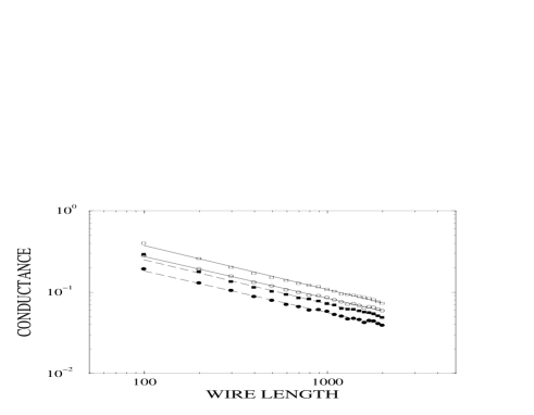
Figure 3: Length scaling of the mean conductance of a wire of 9 (empty circles) or 19 channels (empty squares) at the band center ($E=0$). Average conductances are given in units of the conductance quantum ${e^{2}}/h$ and fitted to power law curves of exponents $-0.51\pm 0.01$ and $-0.54\pm 0.01$, respectively. Filled symbols give the values of the variance obtained for the same sets of randomly generated samples. Dashed lines are just 2/3 of the previous fits. Error bars are of the order of the symbols representing the averages.

The first aim has been the recovery of some important results obtained for wide wires by Mudry, Brouwer, and Furusakimudry . In particular, the exotic dependence of the scaling law on the parity of the wire width is obtained for the present model (a simplification of their Random Flux Model). Open boundary conditions have been used to get conductances of stripes of fixed width and number of open channels (the wire width is equal to the number of channels at the band center). Sample lengths have been varied from 99 to 1980 in steps of 99. As many as $10^{4}$ samples are necessary to get good values of means and other central values of conductance distributions. Fig. 3 shows the scaling law for two typical odd widths (9 and 19 channels) in a log-log plot. Error bars are comparable to the symbols representing the conductance averages. A power law fit to the numerical data is compatible with a mean conductance scaling proportional to the inverse square root of the sample length $L$:

$$<G>\sim{1\over{\sqrt{L}}}.$$

This is precisely the scaling law obtained in Ref.(mudry, ) for quantum wires of an odd section. Notice that scaling proceeds smoothly without distinguishing odd and even wire lengths. As noted by these authors, the variance of the conductance distribution is as large as its mean, making the mean a poor characteristic of the whole distribution. Actually, the predicted relationship

$${<G^{2}>\over<G>}=\frac{2}{3}$$

is accurately reproduced by the numerical data (see filled symbols of Fig. 3 and the dashed lines that are simply $2/3$ of the previous fits). On the other hand, when an even number of channels is studied, exponential scaling of the average conductance together with an exponentially small typical deviation is obtained in complete agreement with previous workmudry .

A deeper understanding of scaling of the conductance mean value can be obtained from the analysis of the whole conductance distribution. Here, conductances for $10^{5}$ samples of width $9$ and lengths $10^{2}$, $10^{3}$, and $10^{4}$ have been compiled and the corresponding histograms plotted in Fig. 4. It is clear that the probability for large values of the conductance diminishes as the length of the wire increases. Actually, since the plot is semilogarithmic the roughly equal separation between filled and empty circles for one side and between empty circles and diamonds for the other side, implies a power law decrease of the probability. The weight that the probability distribution loses for large conductance values goes close to $G=0$. I have checked that the divergence of the probability at $G=1$ is proportional to $1/\sqrt{1-G}$ while the divergence at the origin looks also algebraic but with an exponent starting close to $-{\frac{1}{2}}$ for small disorder and decreasing towards $-1$ as disorder increases.

Although the conductance corresponding to ideal (non disordered) wires equals their widths (9 and 19, in this case), Fig. 4 shows that conductance just reaches the value of 1 for disordered systems. It seems that just one channel is effective. Therefore, it is tempting to compare these conductance distributions with the one corresponding to one random channel within the orthogonal universality classcoe arguing that before localization the effect of disorder is just randomizing transport coefficients. But the comparison is very bad since apart for small differences all theories show probabilities that continuously decrease from $G=0$ to $G=1$. In particular, the simplest result that applies to a random channel described by scattering matrices of the Circular Orthogonal Ensemble is:

$$p(G)=\frac{1}{2\sqrt{G}}\qquad,$$ (9)

that is quite different from the one obtained by numerical simulation. There is a direct mathematical reason explaining this failure. Typically, several states contribute to the Green function calculated at an arbitrary energy within the spectrum of a disordered system. But this is not the case when the Green function of a chiral system is calculated at $E=0$ which is an eigenenergy of the isolated system with an odd number of sites. In this situation, both the Green function of the isolated finite system and the one corresponding to the extended system including the leads (and related to the previous one by a Dyson equation) are dominated by the pole at $E=0$, that is, are completely determined by the $E=0$ eigenfunction. In the next subsection, I will exploit this feature to analyze the conductance distribution as a consequence of a precise wavefunction statistics. Meanwhile, let us return to the theory of Ref. (mudry, ) to analyze the numerical results.

Mudry, Brouwer, and Furusaki give the following expression for the conductance distribution of wires with an odd number of channels in the localized regime (see Eq. (4.10) of the second paper of Ref. (mudry, )):

$$p(G)=\sqrt{C\over\pi}{{\exp\{-C[{\rm arcosh}(G^{-1/2})]^{2}\}}\over{G\sqrt{1-G}}}\qquad,$$ (10)

where

$$C={l\over{4L}}{{M^{2}+M-2}\over{M-1}}\qquad,$$ (11)

with $l$ the mean free path, $L$ the wire length, and $M$ the wire width (which coincides with the number of channels at the bandcenter). A second scaling parameter $\eta$ that characterizes the disorder on a microscopic scale does not appear because it vanishes for the random flux model (RFM) and the model studied here (see Section III) is just a special case of RFM modeljav2 . When $C$ is small enough ($C<0.01$) the distribution is very well described by a much simpler expression (error smaller than one percent for $G\neq 0$):

$$p(G)\simeq\sqrt{C\over\pi}{1\over{G\sqrt{1-G}}}$$ (12)

which allows the evaluation of the mean and the variance of the distribution:

$$<G>\simeq 2\sqrt{C\over\pi}$$

$$<G^{2}>=\frac{2}{3}<G>\qquad.$$

Using the explicit form of $C$ (Eq.(11)) an expression is obtained that can be used to fit the remaining parameter $l$ once an enough number of widths and/or lengths have been studied:

$${<G>}^{2}L\simeq{l\over\pi}{{M^{2}+M-2}\over{M-1}}\qquad.$$ (13)

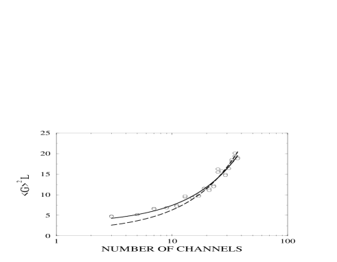
Figure 5: Dependence of the mean conductance and variance on the number of channels for a fixed length of 2000. The number of samples used to get accurate values of the statistical values is $10^{4}$. Two fits to the data are shown: one using Eqs. (4.11a) and (4.11b) of the second paper in Ref.(mudry, ) with $l=1.646$ (dashed line) and a linear fit ($C$ given by Eq.(15)) (continuous line).

Fig. (5) shows a fit to the mean and variance values obtained for sets of $10^{4}$ randomly generated samples of length $L=2000$ and width $M$ from three to 37. While Eq.(13) works reasonably good for large widths it fails near $M=3$. Actually, an alternative fit by a linear law works sensibly better:

$${<G>}^{2}L=aM+b\qquad.$$ (14)

Consequently, the distribution given by Eq. (10) will be used with

$$C=\frac{0.3515M+2.3050}{L}$$ (15)

to describe the results obtained by numeric simulation.

Probability $p(G)$ is shown in Fig. 4 as continuous lines. Although the three numerical distributions are nicely reproduced, accuracy is better for wider wires as expected from the theory ($M\ll L$ is assumed in the theory leading to Eq. (10)). The divergence at $G=1$ is of the inverse square root form while the apparent $G^{-1}$ non–integrable divergence at the origin is regularized by the complex numerator which vanishes at $G=0$. In conclusion, Eq.(10) is a very good description of the numerical data once the constant $C$ is properly estimated.

Let us try an alternative way of characterizing the central value of distributions of the form shown in Fig. 4. Previous experience with disorder models of this kind proves that the median is more robust than the mean for some distributions showing large $G$ variances but smaller $\ln(G)$ variances, i.e., when geometric mean does it better that the usual arithmetic meanjav2 . Unfortunately, the distribution of $\ln(G)$ is also very broad in the present case. Scaling results for the toy model of Section II suggest the use of the median. Fig. 6 gives the median scaling obtained for the previously collected conductance distributions. In can be seen that median values are exponentially smaller than mean values at large wire lengths. The fact that the median scales towards 0 can be inferred from the scaling of the histograms given in Fig. 4 although, the accumulation near exponentially small values of $G$ is not visible in the Figure. Even the scaling law of medians is the same that describes the chain model (see, Eq. (7)). Alternatively, the exponential decay of the median as a function of the square root of the wire length can be inferred from Eq. (10) once the distribution is written as a logarithmic normal distribution using the variable change described in the next subsection.

The practical meaning of the result is quite clear, more than half of the conductance observations are exponentially decreasing as the wire length increases. Actually, the fraction of the samples showing exponentially small conductances increases with wire length because probability below $G=1$ decreases monotonically. Just the difference with a conventional one–dimensional scaling (as, for example, the one obtained for wires of even width) comes from the power law decrease of the upper part of the probability distribution that should be compared with the exponential decrease characteristic of standard scaling.

V.2 Two dimensional system

While a standard study of the scaling of the conductance in 2D would imply the calculation of conductances of increasing $L\times L$ samples connected to ideal leads of width equal to the square side $L$, in this work I have used a dot setup specially designed for the study of just one conducting statenote1 . Certainly, when the number of incoming channels is fixed by a point contact geometry, the only factor that affects the value of the conductance is the size (area) of the dot. In this way, the presumably increase of the conductance due to wider contacts does not obscure the underlying scaling law strictly due to the increased size of the system. Two different limits are well known for large values of $L$. First, ballistic transport through the sample can occur as it happens in chaotic cavities. This limit is described in a first approximation by scattering matrices of the Circular Orthogonal Ensemble (COE)coe . Roughly speaking, a conductance about $1\over 2$ per channel can be expected. Second, Anderson exponential localization would imply an exponentially small value of conductances for large enough dot sizes. This limit applies to diagonal disorder, for example. At the band center of a system with chiral symmetry, numerical simulation shows a behavior similar to the ballistic one (see Fig. 7). Mean conductance converges to a well–defined finite limit while the whole conductance distribution is perfectly described by Eq. (10). Since now the system is not quasi–onedimensional as wide wires are, one is forced to conclude that there should be deep general reasons for the validity of Eq. (10) in this context.

Let me briefly describe the numerical procedure. The transmission between any couple of points within the dot is calculated and the corresponding conductance distribution obtained. To this end, two clean infinite chains (the leads) are attached through two arbitrarily chosen lattice sites within the disordered square sample (the dot). For this geometry, the transmission from site $\bf r$ to site $\bf r^{\prime}$ is given by the following expression:

$$T={{4\ {\psi(\bf r)}^{2}\ {\psi(\bf r^{\prime})}^{2}}\over\big{(}{\psi(\bf r)}^{2}+{\psi(\bf r^{\prime})}^{2}\big{)}^{2}}\qquad,$$ (16)

where $\psi(\bf r)$ is the wavefunction at the band center. From this equation, $0\leq T\leq 1$, and the conductance is between zero and one quantum unit for this numerical simulation. While the large number of transmission evaluations ($\sim\frac{1}{2}L^{4}$) allows for a very precise calculation of the whole conductance distribution, the dependence of the conductance on the separation between point contacts is not given by the procedure. The eigenstate at the band center is obtained by direct inversion of the Schrödinger equation ($\hat{H}\psi=0$) where $\hat{H}$ is given by (8). Once the $E=0$ wavefunction statistics is known, Eq. (16) can be used to get a conductance distribution. For example, if the Porter-Thomas formpoto were valid:

$$f(t)={1\over{\sqrt{2\pi t}}}\exp(-t/2)\qquad,$$ (17)

where $t=N{\psi(\bf r)}^{2}$ being $N$ the number of sites, the conductance distribution would be given by:

$$p(G)=\int_{0}^{\infty}\int_{0}^{\infty}{dt\ dt^{\prime}\ f(t)\ f(t^{\prime})\ \delta\Big{(}G-{{4tt^{\prime}}\over(t+t^{\prime})^{2}}}\Big{)}\qquad.$$ (18)

which can be integrated to give the final result:

$$p_{\rm PT}(G)={1\over\pi}{1\over\sqrt{G(1-G)}}\qquad.$$ (19)

Although probability $p_{\rm PT}(G)$ reproduces some features of the conductance distributions shown in Figs. 4 and 7 for the smaller cluster sizes (for example, the square root divergence at $G=1$), it is clearly non comparable to the accurate result given by Eq.(10). What comes as a surprise is the fact that a logarithmic normal distribution of the wavefunction ratios $t/t^{\prime}$ exactly gives the conductance distribution proposed by Mudry et al.mudry . That is, assuming

$$g(x)=\sqrt{\frac{C}{4\pi}}\exp(-\frac{C}{4}x^{2})$$ (20)

being $x=\ln(t/t^{\prime})$, the conductance distribution is given by

$$\int_{-\infty}^{\infty}{dx\ g(x)\ \delta\Big{(}G-{\frac{4}{e^{x}+e^{-x}+2}}\Big{)}}\qquad.$$ (21)

This integral is easily solved giving $p(G)$ of Eq.(10) with

$$G=\frac{4}{e^{x}+e^{-x}+2}$$

or equivalently,

$$\frac{x}{2}={\rm arcosh}(G^{-1/2})\qquad.$$

This result gives some clue over the complicate $G$ dependence that happens to appear in its distribution function. Numerical simulation (see Fig. 8) shows that Eq.(20) accurately describes the wavefunction squared ratios of large disordered two-dimensional systems and, consequently, conductance distributions of the form given by Eq.(10) are valid in this case.

Let us now discuss the scaling properties of the mean conductance at the band center. Conductance has been averaged over a significant number of randomly generated samples of increasing linear sizes ($L$) keeping almost constant the total number of measurements. Fig. 9 shows the results obtained by this numerical procedure. The scaling of the mean conductance can be fitted to a model of the form:

$$<G>=a+bL^{-\frac{1}{4}}$$ (22)

with a very good precision. The asymptotic value corresponding to the infinite limit is 0.245. Finite values of the conductance of two–dimensional systems showing chiral symmetry have been predicted in a number of papersgade ; furusaki ; mudry0 ; campos ; mudry2 . Although, the present numerical simulation nicely supports these theories some caution must be used for two main reasons. First, a somewhat practical reason. Results heavily depend on the fact that the Green function of this problem is just given by only one particular state. While the energy of this state is well defined theoretically, it could be difficult to make an experiment at just a particular energy. Previous authors on the subject have clearly shown that chirality is lost as soon as $E=0$ is leftmudry . Second reason is a bit more technical. Scaling properties have been obtained for clusters of an odd number of sites and, therefore, a state at $E=0$. Present computational facilities do not allow to prove that scaling of clusters of an even number of states proceeds in the same way. (Note that in this case the Green function should be recalculated for any new position of the point contacts since storing of the whole Green function matrix of the isolated cluster is not possible). Nevertheless, I have checked that odd/even differences are minimal for small systems.

The universal conductance distribution at the band center of a two–dimensional chiral system shown by the thick line in Fig.(7) is probably the most original result in the paper. It corresponds to the $L\to\infty$ limit of Eq.(22) which is obtained for $C=0.0471$ in Eq.(10) but does not differ very much from the distributions corresponding to the simulated sizes ($L=599,699,799$) plotted as three thin indistinguishable lines. All three are accurately described by Eq.(10) with $C=0.0948$. Although obtained for point contacts, previous experience with wide wires proves that minor differences should be expected for wider but finite contactsnote2 . Let me insist in the idea that perfect agreement with the theoretical conductance distribution is also explained by a particular distribution of wavefunction weight ratios (see Eq.(20)) that is confirmed by numerical simulation. Fig. 8 give the distributions obtained for a small cluster size ($L=99$) -higher maximum value- and for a larger size ($L=499$) together with its corresponding Gaussian (dashed line). The thick line gives the universal prediction for this statistical measure of the wavefunction. Consequently, I think that unusual phenomena as they have been described in the literature are quite compatible with present results for the conductance distributionfurusaki ; mudry2 ; campos .

VI Discussion

The scaling properties of the conductance distribution of wide wires showing chiral symmetry has been analyzed by numerical solution of a simple model Hamiltonian. Predictions of a power law decrease of the mean conductance have been confirmed. Besides, the strange scaling properties of the distribution give rise to unusual statistical properties that have been described in the main text. For example, while the slow algebraic decay of the mean conductance is due to few but very large fluctuations, it has been shown that almost all conductance measurements are exponentially small for large wires. Actually, an exponential law is obtained for the median of the distribution and for any generalization of the median based on the integral of the distribution. Nevertheless, exponential decay is not proportional to the sample length but to its square root. That is a significant deviation from standard localization theory.

Surprisingly, statistical conductance properties of two–dimensional systems connected to point contacts are described at the band center by the same distribution that describes wide wires. It has been shown that this statistics appears due to the existence of an underlying Gaussian distribution of the logarithm of the ratio of the wavefunction weights at $E=0$. The main difference with quasi one–dimensional systems is that now both the mean and the median conductance seem to reach a finite limit. The universal statistical distributions of conductance and wavefunction ratios have been obtained. Although they share some properties with the corresponding statistics of the Circular Orthogonal Ensemble, it has been shown that they differ. This numerical result calls for some theory able to explain the origin of such a simple statistics of the wavefunction at the band center of a chiral system.

Figure 1: Length scaling of the conductance of a disordered chain at $E=0$. Average conductance is given in units of the conductance quantum ${e^{2}}/h$. Although the variance of the conductance distribution is large, the values given for the averages show error bars that are sensibly smaller than the symbols representing the mean values. The fit at large lengths by a power law curve of exponent $-0.51\pm 0.01$ is also shown.

Figure 6: Length scaling of the conductance of a wire of 9 (circles) or 19 channels (squares) at the band center ($E=0$). Scaling of the median (filled symbols) is shown besides the data of Fig. 3 in a semilogarithmic plot. Medians can be fitted over the whole range of studied lengths by (7) giving values of $\xi$ equal to 5.73 and 8.99 for the 9 and 19 channels wires, respectively.

Figure 7: Probability distribution of conductances between point contacts in a large disordered square sample. Results for three sizes ($L=599,699,799$) are given together with the theoretical prediction given by Eq. (10) with $C=0.0948$ (All four lines are seen as the thin line in the figure). The universal distribution corresponding to the infinite two–dimensional system is given by the thick line ($C=0.0471$). The conductance distribution corresponding to the Porter-Thomas wavefunction statistics is given by the dashed line. Conductance unit is ${e^{2}}/h$.

Figure 8: Probability distribution of the wavefunction weight ratio in a square disordered dot. Results for two sizes ($L=99$ and $499$) are given as continuous lines together with the theoretical prediction (Eq. (20)) for $C=0.09124$ which corresponds to $L=499$ (dashed line). The universal distribution corresponding to the infinite two–dimensional system is given by the thick line ($C=0.0471$).

Figure 9: Size scaling of the mean value of the conductance between point contacts in a square disordered dot. Continuous line is a fit of the form given by Eq.(22) with an asymptotic value of $a=0.245$. Conductance is given in units of the conductance quantum ${e^{2}}/h$.

- (1) F. J. Dyson, Phys. Rev. , 1331 (1953).
- (2) G. Theodorou and M. H. Cohen, Phys. Rev. B , 4597 (1976).
- (3) T. P. Eggarter and R. Riedinger, Phys. Rev. B , 569 (1978).
- (4) P. W. Brouwer, C. Mudry, B. D. Simons, and A. Altland, Phys. Rev. Lett. 81, 862 (1998).
- (5) E. N. Economou, Green’s Functions in Quantum Physics (Springer–Verlag, Berlin, 1983).
- (6) C. Mudry, P. W. Brouwer, and A. Furusaki, Phys. Rev. B 59, 13221 (1999) and Phys. Rev. B 62, 8249 (2000) and P. W. Brouwer, C. Mudry, and A. Furusaki, Physica E 9, 333 (2001).
- (7) A. Altland and B. D. Simons, Nucl. Phys. B 562, 445 (1999); T. Fukui, Nucl. Phys. B 562, 477 (1999); T. Fukui, Nucl. Phys. B 575, 673 (2000); S. Guruswamy, A. LeClair and A. W. W. Ludwig, Nucl. Phys. B 583, 475 (2000); M. Fabrizio and C. Castellani, Nucl. Phys. B 583, 542 (2000); A. M. Garcia-Garcia and J. J. M. Verbaarschot, Nucl. Phys. B 586, 668 (2000); B. Klein and J. J. M. Verbaarschot, Nucl. Phys. B 588, 483 (2000); T. Guhr, A. Müller-Groeling and H. A. Weidenmüller, Phys. Rep. 299, 189 (1998).
- (8) If the complex probability distribution of selfenergies implied by Eq.(4) were substituted by its geometric mean, a value of 1 would be obtained. But this does not imply that perfect transmission () or diverging localization length in the language of other authors is the average value of the relevant transport magnitude. Actually, both the distribution of selfenergies or Lyapunov exponents are broad and cannot be substituted by any central value of their distributions. Ref. (altshuler, ) further illustrates this point.
- (9) L. I. Deych, A. A. Lisyansky, and B. L. Altshuler, Phys. Rev. Lett. 84, 2678 (2000).
- (10) R. Kubo, J. Phys. Soc. Japan , 570 (1957); R. Kubo, S.J. Miyake, and N. Hashitsume, in Solid State Physics, edited by H. Ehrenreich and D. Turnbull (Academic Press, New York, 1965), Vol. 17, pp. 269–364.
- (11) J. A. Vergés, Phys. Rev. B 57, 870 (1998).
- (12) J. A. Vergés, Comput. Phys. Commun. 118, 71 (1999).
- (13) H. U. Baranger and P. A. Mello, Phys. Rev. Lett. 73, 142 (1994) and Phys. Rev. B 54, R14297 (1996), V. N. Prigodin, K. B. Efetov and S. Iida, Phys. Rev. Lett. 71, 1230 (1993), R. A. Jalabert, J-L. Pichard and C. W. J. Beenakker, Europhys. Lett. 27, 255 (1994), E. McCann and I. V. Lerner, J. Phys.: Condens. Matter 8, 6719 (1996).
- (14) C. E. Porter and R. G. Thomas, Phys. Rev , 483 (1956).
- (15) A conventional scaling analysis like the one followed in Ref.(jav2, ) shows an almost constant conductance average close to quantum units of conductance for clusters sizes from to and both periodic and open boundary conditions.
- (16) R. Gade, Nucl. Phys. B 398, 499 (1993); R. Gade and F. Wegner, ibid. 360, 213 (1991); see also, S. Hikami, M. Shirai, F. Wegner, Nucl. Phys. B 408, 413 (1993); D. K. K. Lee, Phys. Rev. B 50, 7743 (1994).
- (17) A. Furusaki, Phys. Rev. Lett. , 604 (1999).
- (18) A. W. W. Ludwig, M. P. A. Fisher, R. Shankar, and G. Grinstein, Phys. Rev. B 50, 7526 (1994); C. Mudry, C. Chamon, X.-G. Wen, Nucl. Phys. B 466, 383 (1996); I. I. Kogan, C. Mudry, and A. M. Tsvelik, Phys. Rev. Lett. 77, 707 (1996); C. de C. Chamon, C. Mudry, and X-G. Wen , Phys. Rev. Lett. 77, 4194 (1996); Y. Hatsugai, X.-G. Wen, M. Kohmoto, Phys. Rev. B 56, 1061 (1997).
- (19) Situation quantitatively changes when contacts of the order of the square side are considerednote1 . In this case, the conductance average is larger () and its distribution Gaussian.