Bose-Einstein transition in a dilute interacting gas.

Abstract

We study the effects of repulsive interactions on the critical density for the Bose-Einstein transition in a homogeneous dilute gas of bosons. First, we point out that the simple mean field approximation produces no change in the critical density, or critical temperature, and discuss the inadequacies of various contradictory results in the literature. Then, both within the frameworks of Ursell operators and of Green’s functions, we derive self-consistent equations that include correlations in the system and predict the change of the critical density. We argue that the dominant contribution to this change can be obtained within classical field theory and show that the lowest order correction introduced by interactions is linear in the scattering length, $a$, with a positive coefficient. Finally, we calculate this coefficient within various approximations, and compare with various recent numerical estimates.

I Introduction

A precise description of the role of interparticle correlations on the Bose-Einstein transition is indispensable to understanding its physical nature; indeed, correlations are expected to play an essential role in the very existence of superfluidity and related properties, vortices, flow metastability, etc. In general, dilute systems offer the possibility of accurate microscopic treatments. The study of the Bose-Einstein transition in very dilute gases could provide experimental tests of the theory. A large portion of the literature on the modification of the transition temperature is based on a simple transposition of one of the most popular method of condensed matter physics, mean field theory in various guises, where the correlations are unmodified by the interactions and remain purely statistical (as in an ideal gas). Mean field theories, for instance Gross-Pitaevskii, successfully describe a broad variety of interesting phenomena observable in experiments, for example the spatial distribution of the gas in a harmonic trap [1, 2]; for a recent review of numerous successful applications of mean field theories in Bose-Einstein condensation in atomic gases, see [3]. Our purpose in this paper is to go beyond mean field theories and to explore the effects of correlations on the properties of the transition, studying in particular how they modify the transition temperature.

We assume that the interparticle interaction can be described by a positive scattering length $a$, equivalent to the interaction of hard spheres of diameter $a$. We shall also consider a dilute gas, i.e., work in the regime where $a$ is much smaller than the interparticle distance, $an^{1/3}\ll 1$, where $n$ is the particle density. The critical number density, $n_{c}^{0}$, of an ideal gas is given by

$$n_{c}^{0}\lambda^{3}=\zeta(3/2)\simeq 2.612,$$ (1)

where $\lambda$ is the thermal wavelength

$$\lambda=\frac{h}{\sqrt{2\pi mk_{B}T}},$$ (2)

$\zeta$ the Riemann zeta function; $m$ the particle mass and $k_{B}$ Boltzmann’s constant. Note that since at the transition $\lambda\sim n^{-1/3}$, the diluteness condition is equivalent to $a\ll\lambda$.

In an interacting gas, the critical value of the degeneracy parameter, $n_{c}\lambda^{3}$, is modified; the first order change in the critical temperature is related to that in the degeneracy parameter by

$$\frac{\Delta T_{c}}{T_{c}^{0}}=-\frac{2}{3}\frac{\Delta(n_{c}\lambda^{3})}{n_{c}^{0}\lambda^{3}}.$$ (3)

Because mean field theories effectively treat physical systems as ideal gases with modified parameters, the dimensionless degeneracy parameter keeps exactly the same value as in an ideal gas. To calculate its change as a function of the interactions it is necessary to go beyond mean field theories and include correlations arising from the interactions.

One might expect repulsive interactions to increase the degeneracy parameter – equivalently, to decrease the critical temperature, $T_{c}$, at constant density; in general, the presence of hard cores tends to impede the motion of the particles necessary for quantum exchange effects, therefore reducing the influence of quantum statistics and the critical temperature. For example, the superfluid transition temperature of liquid ⁴He is below that of an ideal gas of the same density. Moreover, applying pressure to liquid ⁴He effectively increases the role of the repulsive core of the potential, and decreases the critical temperature.

Studies on the effect of interactions on the transition began in the 1950’s with the work of Huang, Yang, and Luttinger [5], who concluded that the phase transition of the interacting Bose gas “more closely resembles an ordinary gas-liquid transition than the Bose-Einstein condensation,” but they did not make a specific prediction for the change in $T_{c}$. Shortly thereafter Lee and Yang [6] predicted an increase of $T_{c}$ proportional to $a^{1/2}$; later, in Ref. [7] they corrected this result and concluded that the shift of the critical temperature is linear in $a$, with no prediction for the magnitude or even the sign of the effect. In 1960, Glassgold et al. predicted again a positive temperature shift proportional to $a^{1/2}$ [8]. Later, Huang predicted an increase $\sim a^{3/2}$ [9], and recently [10], he predicted that $T_{c}$ increases as $a^{1/2}$, using the same virial expansion as that of Ref. [6]. Despite the lack of qualitative agreement among these many solutions of the problem, these studies showed that the changes in question were not merely due to excluded volume effects (proportional to the cube of the hard core diameter $a$) but to more interesting quantum effects, proportional to a smaller power of $a$.

The problem lay dormant for two decades until it was revisited by Toyoda [11], who studied the transition in the Bogoliubov approximation in the condensed phase. This work predicted a decrease of the critical temperatures at constant density proportional to $a^{1/2}$. As the sign agreed with the measurements in liquid ⁴He, the question appeared settled. Toyoda’s result was reinforced by numerical Path-Integral Quantum Monte Carlo calculations showing that the effect of interparticle repulsion was indeed to decrease the critical temperature [12, 13]. Nevertheless, at the time of these calculations, the issue did not have the same experimental interest as it has now, and it was not fully appreciated that these calculations were limited to relatively high densities and did not explore the region of dilute systems.

With the prospect of experimental realization of Bose-Einstein condensation in dilute gases, Stoof [14, 15] carried out many-body and renormalization group analyses concentrating on the dilute regime. Stoof’s work contains interesting precursors to the present work, e.g., Ref. [14] predicts a linear positive shift in the critical temperature about twice that of our estimate in [16]. Reference [15] predicts more structure in the $a$ dependence of the effect, $\sim a\ln a$, [17], qualitatively similar to the $a^{2}\ln a$ we describe below [18].

A surprise came when the Monte Carlo calculations for hard sphere bosons were extended to lower densities and showed, in addition to the depression of $T_{c}$ at high densities, the existence of a low density regime where the critical temperature is indeed increased by the interaction [19]. At very low densities the shift of the critical temperature was found to be

$$\frac{\Delta T_{c}}{T_{c}^{0}}=c\,n^{1/3}a,$$ (4)

with $c\simeq 0.34$, determined by a numerical extrapolation to the limit $a\to 0$. However, a more recent explicit Monte Carlo calculation [20] of the leading correction to the ideal gas behavior predicts a prefactor $c\simeq 2.3$. One source of the discrepancy lies in the non-analytic dependence of $T_{c}$ on $a$, discussed below, which gives rise to non-linear corrections at the densities where the Monte Carlo calculation of Ref. [19] was performed.

In the past several years, the problem was attacked by analytic approaches based on self-consistent non-linear equations derived both in the Ursell operator formalism [21], and the Green’s function formalism [16]. One finds in both approaches that the effect of repulsive interactions is to decrease the degeneracy parameter, thus increasing the critical temperature at constant density. Moreover, Ref. [16] proves the linearity of $\Delta T_{c}$ in $a$. This was done by observing that the dominant contribution to the shift in the critical density can be calculated by restricting the propagators to their zero Matsubara frequency sector, thereby reducing the quantum many-body problem to a classical field theoretical problem in three spatial dimensions. An alternative proof of the linearity in $a$ based on renormalization group arguments is presented in [22]. While Refs. [21, 16, 22] all agree on the functional form, they do not provide definitive quantitative predictions for the prefactor; Ref. [21] provides $c\sim 1$, and an estimate in Ref. [16] of an exact formula for $\Delta T_{c}/T_{c}^{0}$ predicts $c\sim 2-3$. In the limit of a large number $N$ of components [22], $c=8\pi/3\zeta(3/2)^{4/3}\simeq 2.33$; interestingly, this exact result for $N\to\infty$ agrees with the numerical result $c=2.33\pm 0.25$ of Ref. [20] for $N=2$. The reduction of the problem to classical field theory has been exploited in the recent calculations of the transition in classical $\phi^{4}$ field theory on the lattice extrapolated to the continuum [23, 24], which give $c\simeq 1.3$.

The linearity in $a$ is a non-trivial, non-perturbative result. Since the interaction is itself linear in $a$, one might imagine deriving this result in some form of simple pertubation theory. However, the first order term in $a$, for fixed density, vanishes identically, while all higher order terms have infrared divergences. Nonetheless, various authors have attempted to skirt the infrared problems. For example, Ref. [25] unjustifiably “regularizes” divergences in sums that appear at the transition with an analytic continuation of the Riemann zeta function. Similarly, Ref. [10] uses a virial expansion, unjustified at the critical point, as we discuss below. In another approach, Ref. [26] attempts to exploit differences in first order pertubation theory between the canonical and grand-canonical ensembles in finite volume; this pertubative approach necessarily fails in the thermodynamic limit, preventing a direct determination of the critical temperature. In Ref. [27] finite-size-scaling is used to reconcile this approach with the grand-canonical calculations. Reference [28] calculates $T_{c}$ with the help of an “optimized linear delta expansion , which avoids infrared divergencies and operates for any $N$; for $N=2$ the authors find $c\sim 3.0$, but the validity of the method is difficult to assess, and the accuracy of this result may be affected by uncontrolled errors.

The aim of this paper is to summarize current understanding of the problem of the transition temperature. We provide a more detailed account of our earlier analytical calculations, and in addition compare the Green’s function and Ursell calculations. The paper is organized as follows: In the next section we recall features of the Bose-Einstein transition in an ideal gas and show how the addition of a mean repulsive field does not alter the critical value of the degeneracy parameter. Then in Sec. III we include correlations and obtain, using alternatively the Ursell and Green’s function formalisms, simple self-consistent equations which reveal the physical origin of the change in the critical temperature. In Sec. IV we show that the dominant contribution to the change in the critical temperature can be calculated using a classical field approximation, and we show that the resulting change is linear in the scattering length. Section V is devoted to numerical calculations of the coefficient $c$, and to a numerical exploration of the range of validity of the linear behavior. We focus throughout on a spatially uniform system; a discussion of the transition temperature of a dilute gas in a trap can be found in Refs. [2, 29, 30]. For experimental data in the ⁴He-Vycor system, see [31].

II Ideal gas, mean field and related calculations

In a homogeneous system, the number density of a non-condensed ideal Bose gas is given by

$$n=\int\frac{d^{3}k}{(2\pi)^{3}}\frac{1}{e^{\beta(\varepsilon_{k}^{0}-\mu)}-1}=\frac{1}{\lambda^{3}}g_{3/2}(z)$$ (5)

with $\beta=1/k_{B}T$, $\mu$ is the chemical potential, $z=\exp(\beta\mu)$ the fugacity, and ($\hbar=1$)

$$\varepsilon_{k}^{0}=k^{2}/2m;$$ (6)

the Bose (polylogarithmic) function $g_{p}(z)$ is defined by

$$g_{p}(z)\equiv\sum_{j=1}^{\infty}\frac{z^{j}}{j^{p}}.$$ (7)

As $\mu$ tends to zero from negative values $g_{3/2}(z)\to\zeta(3/2)$ corresponding to the maximum density for a non-condensed gas at a given temperature given by Eq. (1).

The simplest way to include repulsive interactions is in mean field. Assuming that all the effects of interactions can be described by an $s$-wave scattering length, one can generalize Eq. (5) by writing:

$$n=\frac{1}{\lambda^{3}}g_{3/2}(e^{\beta(\mu-\Delta\mu)})$$ (8)

where the shift of the chemical potential $\Delta\mu$ is proportional to the number density:

$$\beta\Delta\mu=2gn\beta=4a\lambda^{2}n,$$ (9)

and $g=4\pi\hbar^{2}a/m$. Equation (8) is a simple consequence of the Hartree-Fock approximation, using a pseudopotential proportional to $a$, in which the shift of the single particle energies is given by

$$\Sigma_{HF}=2gn;$$ (10)

the factor of two comes from exchange. Since $\Sigma_{HF}$ is independent of momentum we have to increase the chemical potential by $\Delta\mu=\Sigma_{HF}$ to keep the same particle density as the ideal gas. The same results are obtained in §4 of Ref. [21].

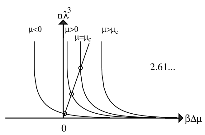
FIG. 1.: Plot of the density $n\lambda^{3}$ as a function of the shift of the chemical potential $\beta\Delta\mu$, for different values of the chemical potential $\beta\mu$. For a given value of $\beta\mu$, the self-consistent solution is given by the intersection point (circle) of this curve with the straight line $\beta\Delta\mu=4a\lambda^{2}n$.

Because the Hartree-Fock self-energy depends on the density, the relation between the chemical potential at the transition and the critical density is more complicated than in the non-interacting case, and the equation $\mu-\Delta\mu=0$ is non-linear. Its solution is conveniently obtained with the geometrical method of [21], illustrated in Fig. 1. At fixed $\mu$ and $\beta$, with $\beta\Delta\mu$ as a variable, the density is obtained through (8); then a simple construction provides the value of $\Delta\mu$ corresponding to the transition. Finally, the density as a function of $\mu$ varies as shown in Fig. 2 (full line); it behaves similarly to that of the ideal gas. However, the transition now occurs at a positive value of the chemical potential and the compressibility $(1/n^{2})\partial n/\partial\mu$ is finite, in contrast to the ideal gas where it diverges. As mentioned in the introduction, the critical density remains exactly the same as for the ideal gas, because at the transition $\mu=\Delta\mu$ and thus critical density is given by the same integral as for the ideal gas.

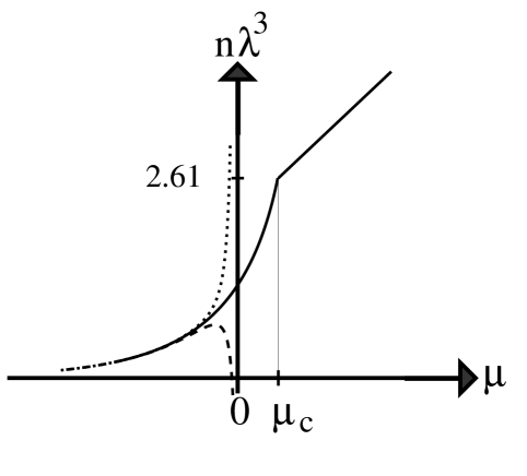
FIG. 2.: Variations of the density $n\lambda^{3}$ as a function of the chemical potential predicted in mean field (full line), for small constant value of the interaction parameter $a/\lambda$. The dotted line corresponds to the ideal gas. The mean field solution curve shows no maximum, but a constantly increasing density as a function of the chemical potential. On the other hand, any finite expansion in orders of $a/\lambda$ leads to divergencies around $\mu=0$ and may introduce spurious extrema (dashed line).

It is instructive to use this simple mean field model to test the limit of simple approximations in an exactly soluble case. Expanding the right side of Eq. (8) in powers of $a/\lambda$ we find the virial expansion:

$$n\lambda^{3}=g_{3/2}(z)-4\frac{a}{\lambda}g_{1/2}(z)\times g_{3/2}(z)+8\left(\frac{a}{\lambda}\right)^{2}g_{3/2}(z)\left\{2\left[g_{1/2}(z)\right]^{2}+g_{3/2}(z)g_{-1/2}(z)\right\}+\dots.$$ (11)

Now, if as Ref. [10] we consider only the first two terms of the expansion we find that the density (the broken lines in Fig. 2) develops a maximum for a negative value of $\mu$; since the density must always be an increasing function of $\mu$, it then becomes tempting to infer that a phase transition should take place at this point. As seen in the figure, this point corresponds to a smaller density than for the ideal gas; this reasoning would then predict an increase of the critical temperature, at constant density, proportional to $\sqrt{a}$, precisely the result obtained in [10]. But one should keep in mind that in this simple model the density maximum is just an artefact of the first order virial expansion, as illustrated by the absence of any maximum in the full curve of Fig. 2; in fact, inclusion of second order terms in $a$ of (11) makes the maximum disappear. From the original Eq. (7), the critical density cannot change. Similar arguments were already given in Refs. [32] and [21]; sufficiently close to $\mu=0$, higher order terms diverge faster and, eventually, dominate the lower order terms in any viral expansion.

The simple example above illustrates the dangers of truncating an expansion in $a$, even within the mean field approximation. The physical origin of the difficulty is simple: the very essence of Bose-Einstein condensation is the appearance of long exchange cycles over the system, which cluster together all particles that they contain [35]; therefore, the phenomenon is not easily captured within any formalism containing a limitation on the size of clusters; further discussion of the effect of long exchange clusters on the position of the Bose-Einstein transition can be found in [19]. One must be very careful in truncating pertubative expansions in which nominally higher-order terms turn out to be of comparable order; rather it is necessary in general to sum an infinite number of terms.

In the calculation of Toyoda [11], the only mean field taken into account is that due to the condensed particles below the transition temperature. His approximation is in fact lowest order Bogoliubov theory. While this theory describes correctly the ground state at zero temperature and its elementary excitations, its extension near the critical temperature meets several difficulties; in particular it predicts a first order phase transition [33], a point not taken into account. In fact, above $T_{c}$, Toyoda’s calculation of the free energy is just that of an ideal gas, with no shift in the critical temperature.

III Self-consistent equations

In this section, as well as in the rest of this paper, we concentrate on the non-condensed state and approach the critical temperature from above. As we have seen in the previous section, mean field effects which produce merely a constant shift in the single particle energies around $T_{c}$ do not affect the value of the critical temperature. A modification of $T_{c}$ thus requires the inclusion of correlations; whose effect of such correlations is to lower the single particle occupation at small $k$. Thus, as the temperature is lowered, the chemical potential reaches the lowest single particle energy for a value smaller than in mean field, resulting in a decrease of $n_{c}$.

It is instructive at this stage to consider the highly oversimplified model in which correlations push down only the level $k=0$ and all other levels are treated within mean field. Then, at the transition, when the $k=0$ level hits the chemical potential, the other particles experience a constant energy shift $\bar{\mu}>0$ with respect to the level $k=0$, and the critical density is given by:

$$n_{c}=\int\frac{d^{3}k}{(2\pi)^{3}}\frac{1}{e^{\beta(\varepsilon_{k}^{0}+\bar{\mu})}-1}=\frac{1}{\lambda^{3}}\,g_{3/2}\left(e^{-\beta\bar{\mu}}\right).$$ (12)

Since $\bar{\mu}$ is small, one can expand the Bose function $g_{3/2}\left(e^{-\beta\bar{\mu}}\right)$:

$$g_{3/2}\left(e^{-\beta\bar{\mu}}\right)=\zeta(3/2)-2\sqrt{\pi\beta\bar{\mu}}.$$ (13)

In fact, in calculating the change in the critical density $\Delta n_{c}=n_{c}-n_{c}^{0}$, one can equivalently expand the statistical factor in (12) at small $k$:

$$\frac{1}{e^{\beta(\varepsilon_{k}^{0}+\bar{\mu})}-1}\to\frac{1}{\beta(\varepsilon_{k}^{0}+\bar{\mu})}$$ (14)

and arrive at the result:

$$\Delta n_{c}=n_{c}-n_{c}^{0}\approx\int_{0}^{\infty}\frac{dk}{\pi^{2}}\frac{m}{\beta}k^{2}\left(\frac{1}{k^{2}+2m\bar{\mu}}-\frac{1}{k^{2}}\right)=-\frac{2}{\lambda^{3}}\sqrt{\pi\beta\bar{\mu}}.$$ (15)

We shall often use the approximation (14) in the following. We note here that it is valid provided only momenta $k\ll\lambda^{-1}$ contribute significantly to the integral (15), which requires $\sqrt{2m\bar{\mu}}\ll\lambda^{-1}$. Since we expect the first correction beyond mean field to be $\beta\bar{\mu}\sim(a/\lambda)^{2}$, this condition is satisfied if $a\ll\lambda$.

As anticipated, the correlations that push down the level $k=0$ lead to a decrease of the critical density, and hence to an increase of the critical temperature. Furthermore, the magnitude of the effect is not necessarily analytic in the small change $\bar{\mu}$ of the chemical potential, and hence in the interaction strength $a$. In fact, the expected result $\beta\bar{\mu}\sim(a/\lambda)^{2}$ together with Eq. (15) lead to $\Delta n_{c}/n_{c}\sim a/\lambda$. To include correlations more generally we consider two approaches, that of Ursell operators used already for this problem in [21], and that of finite temperature field theory. Before deriving detailed results, let us spend a moment comparing the two approaches.

Within finite temperature field theory one typically carries out a systematic expansion of the properties of a many-body system, e.g., the pressure, in powers of the interaction $V$, using either unperturbed Green’s functions $G_{0}$ or self-consistent ones, $G$. Ursell operators provide a different approach to calculating thermodynamic properties of an interacting many-particle system, and lead naturally to expansions in terms of correlations of higher and higher orders. The Ursell operator of rank $n$, $U_{n}$, describes the correlations of a system of $n$ interacting Boltzmann particles. For example, the operator $U_{2}$, defined by

$$U_{2}=e^{-\beta\left(p_{1}^{2}/2m+p_{2}^{2}/2m+V(r_{1}-r_{2})\right)}-e^{-\beta(p_{1}^{2}/2m+p_{2}^{2}/2m)},$$ (16)

acounts for two-body correlations. One expects that matrix elements of $U_{n}$ vanish between states in which one of the particles is far away from the others, and, in the tradition of cluster expansions, one writes expansions of thermodynamic functions in powers of the Ursell operators $U_{n}$. Every term of such an expansions is expected to be finite, even for highly singular potentials such as hard spheres. Inclusion of the specific bosonic or fermionic statistics gives rise to exchange cycles.

Solved exactly, both formalisms give in principle identical results for static thermodynamic properties, and detailed comparisons of how specific approximations can be formulated in either approach can be found in [34]. In the following we study the effects of correlations by means of a simple self-consistent approximation which can be derived in either formalism. This simple self-consistent approximation leads to a nonanalytic change in the spectrum at small $k$.

A Ursell operators

We briefly summarize the principal results obtained in [21] with the Ursell method, reformulated here in a way to make a ready comparision with the Green’s function approach. More details are given in Appendix.

Reference [21] provides the general diagramatic rules to obtain the reduced one-body density operator in momentum space, $\rho_{k}$, as a function of the ideal gas Bose distribution, $f_{k}$, and the Ursell operators $U_{n}$ ($n\geq 2$). Quite generally, above the critical point the single particle density operator has the form of a Bose distribution, but with modified single particle energies,

$$\rho_{k}=f_{k}(\mu-\delta\mu_{k})=\frac{1}{e^{\beta(\varepsilon_{k}^{0}+\delta\mu_{k}-\mu)}-1}.$$ (17)

The particle number density is given in terms of $\rho_{k}$ by

$$n=\int\frac{d^{3}k}{\left(2\pi\right)^{3}}\,\rho_{k}.$$ (18)

When looking for leading order corrections one can safely ignore Ursell operators, $U_{n}$, with $n\geq 3$. The resulting topological structure of the diagrams of the Ursell pertubation series then becomes equivalent to that of the perturbative expansion using Green’s functions with two-body interactions. Furthermore, by treating the matrix elements of $U_{2}$ as momentum independent, one quantitatively recovers the pertubation theory of the Green’s function approach with a momentum-independent coupling constant related to the $s$-wave scattering length $a$. Finally, as we shall below, at the critical point the density operator $\rho_{k}$ becomes large at small momenta, $\rho_{k}\gg 1$ for $k\to 0$, so that the approximation

$$1+\rho_{k}\simeq\rho_{k}\simeq[\beta(\varepsilon_{k}^{0}+\delta\mu_{k}-\mu)]^{-1}$$ (19)

can be used systematically (as in (29) below). These remarks explain why the results that we obtain using Ursell operators will eventually be identical to those obtained within the Green’s function approach in the particular limit of $a\ll\lambda$.

FIG. 3.: (a) First order Ursell diagrams; the double line corresponds to one operator $U_{2}$. Here we slightly change the representation of Ref. [21] and replace the dotted segments there (corresponding to a summation over all exchange cycle lengths) by closed curves; in this way, the $U_{2}$ diagrams become very similar to the usual Green’s function diagrams. Despite this close graphical similarity, the physical interpretation of the diagrams is different: for instance, exchange cycles do not appear at all in Green’s function diagrams. (b) Simplest examples of the diagrams included in the iteration. (c) Diagrams leading to Eqs. (24) and (108). (d) Bubble diagrams leading to Eq. (111).

To obtain the mean field result, Eq. (32) of Ref. [21], we iterate the first order diagrams shown in Fig. 3a (examples of iterated diagrams are shown in Fig. 3b); this leads to:

$$\rho_{k}=f_{k}(\mu-\Delta\mu),$$ (20)

with

$$\beta\Delta\mu\simeq 4a\lambda^{2}\int\frac{d^{3}k}{(2\pi)^{3}}\,\rho_{k}=4a\lambda^{2}n.$$ (21)

In this approximation the only effect of the interactions is to produce a momentum independent shift of the single particle energies which, as discussed in the previous section, can be absorbed in a shift of the chemical potential:

$$\mu^{\prime}=\mu-\Delta\mu,$$ (22)

leaving the critical density identical to that of the ideal gas.

To go beyond mean field, we include in the self-consistent equation for $\rho$ the corrections displayed in Fig. 3c. These are formally of second order in $a/\lambda$ and read (§5 of [21]):

$$\rho_{k}=f_{k}(\mu^{\prime}-\delta\mu_{k}),$$ (23)

with

$$\beta\delta\mu_{k}\simeq-8\left(\frac{a}{\lambda}\right)^{2}\lambda^{6}\int\frac{d^{3}k^{\prime}}{(2\pi)^{3}}\int\frac{d^{3}q}{(2\pi)^{3}}\,\rho_{k^{\prime}}\,\rho_{k^{\prime}-q}\,\rho_{k+q}.$$ (24)

Note how the integral (24), in which momentum conservation appears explicitly ($q$ is the momentum transfer in a binary collision), introduces a $k$-dependence of the energy shift, as opposed to the result of the simple mean field approximation.

We assume that the single particle state with $k=0$ still has the lowest energy, so that the phase transition occurs when

$$\mu^{\prime}-\delta\mu_{k=0}=0.$$ (25)

The critical density is then given by

$$n_{c}=\int\frac{d^{3}k}{(2\pi)^{3}}\,\rho_{k}=\int\frac{d^{3}k}{(2\pi)^{3}}\,f_{k}(\delta\mu_{k=0}-\delta\mu_{k}),$$ (26)

which, because of the $k$-dependence of $\delta\mu_{k}$, does not coincide with the critical density of the ideal gas obtained for constant $\delta\mu$. Instead

$$\Delta n_{c}=n_{c}-n_{c}^{0}=\int\frac{d^{3}k}{(2\pi)^{3}}\,\left[f_{k}(\delta\mu_{k=0}-\delta\mu_{k})-f_{k}(\delta\mu_{k=0})\right].$$ (27)

In general, $\delta\mu_{k}-\delta\mu_{k=0}$ is an increasing function of $k$, so that $\Delta n_{c}$ is negative.

The variable appearing in Eq. (26),

$$\delta\mu_{k}-\delta\mu_{k=0}\simeq-\frac{8}{\beta}\left(\frac{a}{\lambda}\right)^{2}\lambda^{6}\int\frac{d^{3}k^{\prime}}{(2\pi)^{3}}\int\frac{d^{3}q}{(2\pi)^{3}}\,\rho_{k^{\prime}}\,\rho_{k^{\prime}-q}\,\left[\rho_{k+q}-\rho_{q}\right],$$ (28)

can be simplified if we notice that when the critical condition (25) is fulfilled the dominant contribution to the integrals comes from small momenta for which the statitical factors $f_{k}$ diverge. In fact, if the $f_{k}$’s are evaluated with the free particle spectrum, the integral in (24) becomes logarithmically divergent in the infrared. To see that, we expand the $f_{k}$’s as in (14),

$$\left[e^{\beta(\varepsilon_{k}^{0}-\mu^{\prime}+\delta\mu_{k})}-1\right]^{-1}\simeq\frac{1}{\beta(\varepsilon_{k}^{0}+\delta\mu_{k}-\mu^{\prime})}.$$ (29)

Setting

$$\varepsilon_{k}=\varepsilon_{k}^{0}+\delta\mu_{k}-\delta\mu_{k=0},$$ (30)

we obtain the self-consistent relation valid at small $k$,

$$\varepsilon_{k}=\varepsilon_{k}^{0}-8\left(\frac{a\lambda^{2}}{\beta^{2}}\right)^{2}\int\frac{d^{3}k^{\prime}}{(2\pi)^{3}}\int\frac{d^{3}q}{(2\pi)^{3}}\frac{1}{\varepsilon_{k^{\prime}}}\frac{1}{\varepsilon_{k^{\prime}-q}}\left[\frac{1}{\varepsilon_{k+q}}-\frac{1}{\varepsilon_{q}}\right].$$ (31)

A simple power counting argument indicates the integral is logarithmically divergent if we replace the self-consistent energies $\varepsilon$ by the free $\varepsilon_{k}^{0}$. For the self-consistent spectrum, however, no infrared divergences occur, as we shall see in III C.

B Green’s functions

In the normal state the single particle Green’s function $G(k,z_{\nu})$ is given

$$G^{-1}(k,z_{\nu})=z_{\nu}+\mu-\varepsilon_{k}^{0}-\Sigma(k,z_{\nu}),$$ (32)

where $k$ is the single particle momentum, and $z_{\nu}=2\pi i\nu/\beta$ is a Matsubara frequency, with $\nu=0,\pm 1,\pm 2,\dots$. The self-energy $\Sigma(k,z)$, which describes the effect of the interactions, can be obtained as a series in powers of the interaction strength $a$ by standard diagrammatic techniques [4, 37, 38, 39]. The single particle density matrix is related to $G$ by

$$\rho_{k}=-T\sum_{\nu}\,\,e^{z_{\nu}0^{+}}\,G(k,z_{\nu}).$$ (33)

The criterion for condensation is that the chemical potential $\mu$ reaches the bottom of the single particle excitation spectrum, and we again assume, as in §III A, that the lowest single particle state is that with $k=0$. The transition point is then determined by the condition [40]:

$$G^{-1}(0,0)=0\quad\text{or}\quad\Sigma(0,0)=\mu\,.$$ (34)

At that point,

$$G^{-1}(k,z_{\nu})=z_{\nu}-\varepsilon_{k}^{0}-\left[\Sigma(k,z_{\nu})-\Sigma(0,0)\right],$$ (35)

To first order in the interaction strength, the self-energy is given by the Hartree-Fock approximation, leading to a contribution $\Sigma_{HF}$ (see Eq. (10)) independent of both $k$ and $z$ which can then be eliminated by a redefinition of the chemical potential, as discussed above.

FIG. 4.: (a) Green’s function diagrams leading to Eq. (36), similar to Fig. 3c. (b) Green’s function bubble diagrams leading to Eq. (99), similar to Fig. 3d.

The structure of $\Sigma(k,z)$ in next order is described by the two diagrams in Fig.  4a. The second is the exchange term of the first, and within the present approximation in which the matrix elements of the interaction do not depend on momenta, the two contributions are equal. Replacing the free propagators by their Hartree-Fock version, we have

$$\Sigma(k,z_{\nu})=2g^{2}\int\frac{d^{3}k^{\prime}}{(2\pi)^{3}}\frac{d^{3}q}{(2\pi)^{3}}\frac{f_{k^{\prime}}(1+f_{k^{\prime}+q})(1+f_{k-q})-(1+f_{k^{\prime}})f_{k^{\prime}+q}f_{k-q}}{z_{\nu}+\mu^{\prime}+\varepsilon_{k^{\prime}}^{0}-\varepsilon_{k^{\prime}+q}^{0}-\varepsilon_{k-q}^{0}}.$$ (36)

Because the condensation condition (34) involves only the Matsubara frequency $z_{\nu}=0$, we concentrate from now on this contribution. Furthermore, as before, we isolate the dominant contribution by expanding the statistical factors, so that $f_{k}\sim T/\varepsilon_{k}^{0}$, and

$$\Sigma(k,0)-\Sigma(0,0)\simeq-2g^{2}T^{2}\int\frac{d^{3}k^{\prime}}{(2\pi)^{3}}\frac{d^{3}q}{(2\pi)^{3}}\frac{1}{(\varepsilon_{k^{\prime}}^{0}-\mu^{\prime})(\varepsilon_{k^{\prime}-q}^{0}-\mu^{\prime})}\left(\frac{1}{\varepsilon_{k-q}^{0}-\mu^{\prime}}-\frac{1}{\varepsilon_{q}^{0}-\mu^{\prime}}\right).$$ (37)

Replacing the bare energies $\varepsilon_{k}^{0}$ by the dressed energies $\varepsilon_{k}^{0}+\Sigma(k,0)$, observing that $\mu^{\prime}=\Sigma(0,0)$ at the transition, and setting

$$\varepsilon_{k}=\varepsilon_{k}^{0}+\Sigma(k,0)-\Sigma(0,0),$$ (38)

we recover Eq. (31). Note that the earlier $\delta\mu_{k}-\delta\mu_{k=0}$ is simply $\Sigma(k,0)-\Sigma(0,0)$.

C Discussion

The change of the critical density is intrinsically related to $\delta\mu_{k}$ (or equivalently $\Sigma(k,0)$) by Eq. (26). In terms of

$$U(k)=2m\left[\delta\mu_{k}-\delta\mu_{k=0}\right]=2m\left[\Sigma(k,0)-\Sigma(0,0)\right],$$ (39)

the change of the critical density introduced by the interaction is

$$\Delta n_{c}=\int\frac{d^{3}k}{(2\pi)^{3}}\left\{\frac{1}{e^{\beta[k^{2}+U(k)]/2m}-1}-\frac{1}{e^{\beta k^{2}/2m}-1}\right\}$$ (40)

or

$$\Delta n_{c}\simeq-\frac{2}{\pi\lambda^{2}}\int_{0}^{\infty}dk\,\frac{U(k)}{k^{2}+U(k)},$$ (41)

where in the second line we have used the approximation (14).

The heart of the calculation of the critical density is then to determine the function $U(k)$, a non-trivial task, since the evaluation of this function by naive perturbation expansion fails because of infrared divergences. However, higher order iterations lead to an instability in the energy spectrum at small momenta, as in Ref. [21]. In the limit of an infinite number of iterations, the spectrum around $k=0$ hardens: the self-consistent solution of (24) leads indeed to $\varepsilon_{k}\sim k^{3/2}$, as predicted by Patashinskii and Pokrovskii [42] using the following argument.

For free particles, the integral in Eq. (37) contains six powers of momentum in both the numerator and denominator, and is thus logarithmically divergent. In order to ensure that the self-consistent solution, $\varepsilon_{k}$, converges in the infrared limit, $\varepsilon_{k}$ must behave (modulo possible logarithmic corrections) as $\sim k^{\alpha}$ with $\alpha<2$, so that the free particle energies, $\varepsilon_{k}^{0}\sim k^{2}$, can be neglected at small $k$ with respect to $\Sigma(k,0)-\Sigma(0,0)$. With this behavior, $\Sigma(k,0)-\Sigma(0,0)\sim k^{6-3\alpha}$, so that we find a self-consistent energy spectrum, $\varepsilon_{k}\sim\Sigma(k,0)-\Sigma(0,0)\sim k^{\alpha}$, for $\alpha=3/2$.

The modification of the spectrum occurs only for small momenta $k\ll k_{c}$, where $k_{c}$ is a scale that will be specified below. We note here only that since $U(k)$ is of order $a^{2}/\lambda^{4}$, one expects $k_{c}$ to be of order $a/\lambda^{2}$. For momenta $k_{c}\ll k\to\infty$, perturbation theory becomes applicable leading to $U(k)/k^{2}\to 0$. The typical momenta involved in the integral (41) are of order $k_{c}$. The validity of Eq. (41) for $k\ll\lambda^{-1}$ requires $k_{c}\ll\lambda^{-1}$, which is satisfied in the dilute limit.

We later present numerical self-consistent solutions of Eq. (31). Here we reconsider the simple analytical model calculation of Ref. [16] which provides an estimate for the scale $k_{c}$, and acts as a reference for the numerical results presented later. In this analytical model we construct a self-consistent energy spectrum at the critical point:

$$\varepsilon_{k}=\frac{\hbar^{2}k^{2}}{2m}+\Sigma(k,0)-\Sigma(0,0)$$ (42)

within the approximation (37) for the self-energy, which we write as

$$\Sigma(k,0)-\Sigma(0,0)=-2g^{2}T\int\frac{d^{3}q}{(2\pi)^{3}}B(q)\left(\frac{1}{\varepsilon_{k-q}}-\frac{1}{\varepsilon_{q}}\right),$$ (43)

where the bubble diagram contributes

$$B(q)=T\int\frac{d^{3}p}{(2\pi)^{3}}\frac{1}{\varepsilon_{p}\varepsilon_{p+q}}.$$ (44)

To extract the low momentum structure, below the scale $k_{c}$, we evaluate the most divergent terms of Eq. (43) using the following ansatz:

$$\varepsilon_{k}=k_{c}^{1/2}\frac{\hbar^{2}k^{3/2}}{2m}\Theta(k_{c}-k)+\frac{\hbar^{2}k^{2}}{2m}\Theta(k-k_{c}).$$ (45)

With this spectrum, Eq. (44) becomes

$$B(q)\simeq\frac{4m}{\pi\hbar^{2}\lambda^{2}k_{c}}\left[\ln\left(\frac{k_{c}}{q}\right)+c\right],$$ (46)

where $c\approx 2+2\ln 2-\pi/2$ =1.816, and in the limit $k\to 0$ the self-energy is

$$\Sigma(k,0)-\Sigma(0,0)=\frac{1024\pi\hbar^{2}}{15m}\left(\frac{a}{\lambda^{2}}\right)^{2}\left(\frac{k}{k_{c}}\right)^{3/2}.$$ (47)

Identifying the right side of this equation with $k_{c}^{1/2}\hbar^{2}k^{3/2}/2m$, the self-consistency condition, Eq. (45), in the limit $k\to 0$ applies that

$$k_{c}=32\left(\frac{2\pi}{15}\right)^{1/2}\frac{a}{\lambda^{2}}\approx 20.7\frac{a}{\lambda^{2}}.$$ (48)

As expected, the scale of the low momentum structure is $a/\lambda^{2}$. However, one should note that the large value of the numerical factor implies that the range of validity of the calculation is limited to very small values of $a/\lambda$ (so that the condition $k_{c}\ll\lambda^{-1}$ is fulfilled).

The energy spectrum obtained with this analytical model is only self-consistent for wavevectors $k\ll k_{c}$. In the limit $k\gg k_{c}$ we assume that $\varepsilon_{k}$ goes over to the free particle spectrum $\varepsilon_{k}\simeq\hbar^{2}k^{2}/2m$, ignoring here a logarithmic correction (see Sec. V). We smoothly interpolate between these limits, writing

$$U(k)=\frac{2m}{\hbar^{2}}\left(\Sigma(k,0)-\Sigma(0,0)\right)=\frac{k_{c}^{1/2}k^{3/2}}{1+(k/k_{c})^{3/2}}.$$ (49)

Thus we estimate the critical temperature as

$$\frac{\Delta T_{c}}{T_{c}}=\frac{4\lambda}{3\pi\zeta(3/2)}\int_{0}^{\infty}\frac{U(k)}{k^{2}+U(k)}\simeq 3\,an^{1/3}.$$ (50)

While the precise coefficient is sensitive to the details of the interpolation between the low and high $k$ limits, e.g., (49), the result remains of order unity in any case.

The $k^{3/2}$ spectrum is only an approximation and is not stable if higher order corrections are included; from the general theory of phase transitions, at $T_{c}$, $\varepsilon_{k}\sim k^{2-\eta}$, where $\eta=\varepsilon^{2}/54\simeq 0.02$ in an $\varepsilon=4-D$ expansion or $\eta=8/(3\pi^{2}N)\simeq 0.14$ in the large $N$ limit (with $N=2$) [43]. This model provides too strong a modification of the spectrum at small momenta.

The model calculation illustrates however the basic mechanism behind the change of the degeneracy parameter, the modification of the single particle energy spectrum at small momentum. This may be understood as a result of correlations among particles caused by their repulsive interactions: particles minimize their repulsion by avoiding each other in space, i.e., by correlating their positions; the physical origin of the effect is therefore a spatial rearrangement that affects the atoms with low momentum. By contrast, atoms with high momenta have too much kinetic energy to develop significant correlations. The modification of the spectrum translates into a modification of the population of the various levels. In particular the low momentum levels at momentum scale $\sim k_{c}$ are less populated than they would in a mean field approximation at the same density, and the overall result is a decrease of the critical density.

The hardening of the spectrum obtained as a solution of the self-consistent equations, which is responsible for the decrease of the critical density, also provides a cure for the infrared divergences which occur in the perturbative calculation in second order. However, as we shall see in the next section, such divergences appear in all orders in perturbation theory, so that we need a more general scheme to approach the problem.

IV Classical field approximation

In this section we extend the discussion of the previous section in a way that is at the same time more general, in that it is not restricted to any particular class of diagrams, and less general, in that only the linear corrections to the density are investigated.

A Breakdown of perturbation theory

Our main goal is the calculation of the critical density. As an intermediate step, we distinguish in Eq. (33) for $\rho_{k}$ the contribution of zero and non-zero Matsubara frequencies:

$$\rho_{k}=-TG(k,0)-T\sum_{\nu\neq 0}\,G(k,i\omega_{\nu}).$$ (51)

The density is obtained by integrating over momentum $k$ (see Eq. (18)). The terms with $\nu\neq 0$ are regular at small momentum since a non-vanishing Matsubara frequency provides an infrared cutoff. They provide corrections to the density, that are analytic in the self-energy, and therefore of the same order as $\Sigma$, starting at order $a^{2}$ (modulo possible logarithmic corrections). On the other hand, the integral for $\nu=0$ is singular for small $k$, and the infrared divergences introduce non-analyticity in $a$. Since, we are interested here in the dominant correction to the critical density, we will retain only this term in $\rho_{k}$. Note that the resulting expression for the density is ultraviolet divergent, a problem bypassed by calculating the change in the critical density.

As illustrated by the example of the previous section, infrared divergences also occur in the calculation of self-energies $\Sigma(k,0)$; we now use simple power counting arguments to analyze these divergences. Let us first consider diagrams in which all the internal lines carry zero Matsubara frequencies. It is convenient here to introduce a new notation and set

$$\varepsilon^{0}_{k}-\mu^{\prime}=(k^{2}+\zeta^{-2})/2m.$$ (52)

The quantity $\zeta$, a the mean field correlation length, is given by

$$\frac{\hbar^{2}}{2m\zeta^{2}}=-\mu^{\prime}=-(\mu-\Sigma_{HF});$$ (53)

$\zeta$ plays the role of an infrared cutoff in the integrals. Note that $\zeta\rightarrow\infty$ ($\mu^{\prime}\rightarrow 0$) when $T\rightarrow T_{c}^{0}$. In the perturbation series, we take the intermediate propagators to be neither free, nor fully self-consistent as in the previous section, but containing the mean field contributions. All the functions that are integrated in the diagrams then appear as products of fractions of the form

$$\left[K^{2}+\zeta^{-2}\right]^{-1},$$ (54)

where $K$ denotes a generic combination of momenta; it is then natural to use the dimensionless products $K\zeta$ as new integration variables. Consider then a diagram of order $a^{n}$. The lowest order $n=2$ has been already explicitly written in (37), and it is proportional to $(a/\lambda)^{2}\ln(k\zeta)$, where $k$ is the external momentum. For $n>2$, every additional order brings in one factor $a$ from the vertex, one integration over three-momenta, a factor $T$, and two Green’s functions (the internal lines). The contribution of the diagram can thus be written as:

$$T\,\left(\frac{a}{\lambda}\right)^{2}\left(\frac{a\zeta}{\lambda^{2}}\right)^{n-2}F(k\zeta),$$ (55)

where $F$ is a dimensionless function, which we do not explicitly need here. The main point is that when one approaches the critical temperature, the coherence length becomes large so that the summation of terms (55) diverges. In the critical region, $\zeta$ is $\sim\lambda^{2}/a$, so that all the terms in the perturbative expansion are of the same order of magnitude. Therefore, at the critical point, perturbation theory is not valid.

Let us now assume that in a given diagram some propagators carry non-zero Matsubara frequencies so that one momentum integration will be altered. For that integration, the presence of an additional imaginary term $2i\pi\nu T$ in the denominators of the propagators ensures that no singularity at $k=0$ can take place. Essentially, in the corresponding propagators, $\zeta$ is replaced by a term proportional to $\lambda$, so that one factor $a\zeta/\lambda^{2}$ in (55) is now replaced by $a/\lambda$. Compared to the diagram with only vanishing Matsubara frequencies, this diagram is down by a factor $a/\lambda$, and thus negligible in a leading order calculation of $\Sigma$.

B Classical field approximation

The diagrams where all Matsubara frequencies vanish are those of an effective theory for static fields. Ignoring the non-zero Matsubara frequencies is indeed equivalent to ignoring the (imaginary) time dependence of the field operators. In this approximation the many-body problem reduces to a classical field theory in three space dimensions.

The energy of a classical field configuration is given by

$${\cal H}=\int d^{3}r\left(\frac{|\nabla\varphi^{(}r)|^{2}}{2m}-\mu^{\prime}|\varphi(r)|^{2}+\frac{2\pi a}{m}|\varphi(r)|^{4}\right).$$ (56)

The zero Matsubara component of the density is given by $\langle|\varphi(r)|^{2}\rangle$. By assumption, the wavenumbers of the classical field are limited to $k$ less than an ultraviolet cutoff $\Lambda\sim\lambda^{-1}$. As one approaches the critical region, $k\mathrel{\hbox to0.0pt{\raise 2.20013pt\hbox{$<$}\hss}{\lower 2.20013pt\hbox{$\sim$}}}k_{c}$, all the terms in the integrand of (56) become of the same order of magnitude:

$$\frac{k_{c}^{2}}{2m}\sim\mu^{\prime}\sim\frac{a}{m}\frac{T}{\mu^{\prime}}k_{c}^{3},$$ (57)

where $(T/\mu^{\prime})k_{c}^{3}$ is the contribution to the density of the modes with $k\sim k_{c}$. From Eq. (57) we see that $k_{c}\sim a/\lambda^{2}$. For $k\simeq k_{c}$ perturbation theory in $a$ makes no sense, and in fact all terms in the perturbative expansion are infrared divergent. For $k_{c}\ll k\ll\lambda^{-1}$, perturbation theory is applicable. Note that, in the critical region, $\zeta\sim 1/k_{c}\sim\lambda^{2}/a$.

By a simple rescaling of the fields $\varphi\to\sqrt{mT}\phi$, one can write the effective action for the classical field theory as

$$-{\cal H}/T=\int d^{3}r\left(\frac{1}{2}|\nabla\phi(r)|^{2}-m\mu^{\prime}|\phi(r)|^{2}+\frac{4\pi^{2}a}{\lambda^{2}}|\phi(r)|^{4}\right).$$ (58)

The rescaled fields $\phi$ have the dimensions of an inverse length. The classical theory contains ultraviolet divergences, which spoil simple dimensional arguments for the linear change of $T_{c}$.

C Linear dependence of the density correction

We now consider a diagrammatic expansion of $\Sigma$ in terms of the full zero frequency Green’s function, defined by:

$$-2mG^{-1}(k)=k^{2}-2m\mu+2m\Sigma(k,a,G,\Lambda),$$ (59)

from here on we obmit the explicit index $\nu=0$ in $\Sigma$ and $G$. In this self consistent expression the self consistent the self-energy $\Sigma$ depense on $\mu$ only through its dependence on $G$. Instead of $\mu$, we use the dimensionless parameter $\alpha$ defined by

$$-2m\mu+2m\Sigma(0)=\alpha\frac{a^{2}}{\lambda^{4}}.$$ (60)

The parameter $\alpha$ controls the distance to the critical point; it vanishes exactly at the transition, as opposed to $\mu$. In terms of $\alpha$ the Green’s function is now given by:

$$-2mG^{-1}(k)=k^{2}+\alpha\frac{a^{2}}{\lambda^{4}}+U(k),$$ (61)

where

$$U(k)=2m\Sigma(k,a,G,\Lambda)-2m\Sigma(0,a,G,\Lambda).$$ (62)

Since $\Sigma$ depends only on the full Green’s function, $U(k)$ depends only on $\alpha$ and not on $\Sigma(0)$; moreover, the ultraviolet divergence in $\Sigma(k)$ is only logarithmic, and the difference $U(k)$ is independent of the cutoff $\Lambda$ in the limit $\Lambda\to\infty$.

If we assume that $\Lambda\to\infty$, the power counting analysis of §IV A implies that

$$U(k)=\frac{a^{2}}{\lambda^{4}}\,\widetilde{\sigma}\left(\frac{k\lambda^{2}}{a},\alpha\right).$$ (63)

Inserting this result into (41) and making the change of variable $x=k\lambda^{2}/a$, one finds

$$\Delta n_{c}=-\frac{2a}{\pi\lambda^{4}}\lim_{\alpha\rightarrow 0}\int dx\frac{\widetilde{\sigma}(x,\alpha)}{x^{2}+\widetilde{\sigma}(x,\alpha)},$$ (64)

showing that the change in the critical density is indeed linear in $a$.

This result assumes that the limit $\widetilde{\sigma}(x,\alpha\to 0)$ is well defined. This is the case in the self-consistent schemes that we discussed above; they avoid the infrared problem of perturbative calculations, and lead to well defined values of $\Delta n_{c}$. Similarly, in calculations involving resummations of bubbles or ladder diagrams the cutoff is provided by an effective screening explicitly generated by the infinite resummations. Large $N$ techniques lead to a similar screening, with the advantage of also providing an expansion parameter [22, 44].

On the other hand, situations where the limit $\widetilde{\sigma}(x,\alpha\to 0)$ is problematic are encountered in perturbation theory where, for reasons discussed above, an infrared cutoff is needed; determination of this cutoff through the condensation condition can lead to spurious $a$ dependence (an explicit example is worked out in detail in the next section).

The linearity of the shift in the critical density does not depend on the ultraviolet cutoff and is thus an universal quantity. Nevertheless, the universal behavior implicity assumes that the limit $\Lambda\to\infty$ has been taken and is strictly valid only in the limit $a\to 0$. If $a$ is not sufficiently small, the classical field approximation ceases to be valid and non-linear corrections appear. The classical field approximation requires that all momenta involved in the various integrations are small in comparison with $\Lambda\sim\lambda^{-1}$ or, in other words, that the integrands are negligibly small for momenta $k\sim\lambda^{-1}$. Only then, for instance, can we use the approximate form of the statistical factors (29). This requires in particular that $k\sim k_{c}\ll\Lambda$, yielding $a/\lambda\ll 1$. In fact, because, as we shall see, the relation between $k_{c}$ and $a/\lambda$ involves a large number, this regime is reached only for very small values, $a/\lambda\mathrel{\hbox to0.0pt{\raise 2.20013pt\hbox{$<$}\hss}{\lower 2.20013pt\hbox{$\sim$}}}10^{-2}-10^{-3}$.

V Explicit calculations

Our goal in this section is to provide specific illustrations of the discussions of the previous sections. We first present analytical calculations which shed light on the difficulties encountered when attempting to calculate the shift in the critical temperature using perturbation theory. Then we show how partial resummations of the perturbative expansion generate screening of long range correlations and allow an explicit calculation of the self-energy, and then of the transition temperature. Finally we present results of numerical self-consistent calculations, which we compare with the analytical counterparts, and evaluate the limitations of the classical field theory. The accuracy of such approximative schemes is difficult to gauge a priori. An alternative is to use lattice calculations to solve the three-dimensional classical field theory. Results of such calculations have been presented recently [23, 24].

A Second order perturbation theory

In order to illustrate the difficulties that one meets in perturbative calculation near $T_{c}$, let us return for a moment to the second order self-energy diagram, which is the lowest order diagram that introduces correlations and therefore corrections to the critical density. The value of this diagram for vanishing Matsubara frequencies is given by Eq. (37)

$$\Sigma(k)-\Sigma(0)=-2g^{2}T^{2}\int\frac{d^{3}k^{\prime}}{(2\pi)^{3}}\frac{d^{3}q}{(2\pi)^{3}}\frac{1}{(\varepsilon^{0}_{k^{\prime}}-\mu^{\prime})(\varepsilon^{0}_{k^{\prime}-q}-\mu^{\prime})}\left[\frac{1}{\varepsilon^{0}_{k+q}-\mu^{\prime})}-\frac{1}{\varepsilon^{0}_{q}-\mu^{\prime}}\right],$$ (65)

where $g=4\pi a/m$.

We note that $\Sigma(k)$ is the convolution of three factors of the form $1/(k^{2}+\zeta^{-2})$, with $\zeta$ defined in Eq. (53). Using the Fourier transform

$$\int\frac{d^{3}k}{(2\pi)^{3}}\,\frac{\text{{\rm e}}^{ikr}}{k^{2}+\zeta^{-2}}=\frac{1}{4\pi r}e^{-r/\zeta},$$ (66)

we obtain

$$2m\Sigma(k)=-128\pi^{2}\left(\frac{a}{\lambda^{2}}\right)^{2}\int r^{2}drj_{0}(kr)\left(\frac{e^{-r/\zeta}}{r}\right)^{3},$$ (67)

where $j_{0}(x)\equiv\sin x/x$. This expression contains, as anticipated, a logarithmic divergence at small distances. Let us isolate this divergence by separating the Bessel function $j_{0}(x)$ into its value at the origin and a correction term:

$$j_{0}(x)=j_{0}(0)+\left(\frac{\sin x}{x}-1\right)$$ (68)

The first term gives a momentum independent contribution, given by $\Sigma(0)$. Introducing a cutoff $1/\Lambda$ to control the ultraviolet divergence, we obtain

$$2m\Sigma(0)=128\pi^{2}\left(\frac{a}{\lambda^{2}}\right)^{2}\mathrm{Ei}(-\frac{3}{\Lambda\zeta})\approx-128\pi^{2}\left(\frac{a}{\lambda^{2}}\right)^{2}\left[\ln(\frac{\Lambda\zeta}{3})-\gamma\right],$$ (69)

where $\gamma=0.577\ldots$ is Euler’s constant, and $\mathrm{Ei}$ the exponential integral function. The last approximate equality is valid when $\Lambda\zeta\gg 1$, which we assume to be the case. The second term, which is regular and equal to $2m(\Sigma(k)-\Sigma(0))=U(k)$, does not require a cutoff. The result is

$$U(k) = -128\pi^{2}\left(\frac{a}{\lambda^{2}}\right)^{2}\int_{0}^{\infty}(j_{0}(kr)-1)\,\frac{e^{-3r/\zeta}}{r}\,dr\,$$ (70)

$$= 128\pi^{2}\left(\frac{a}{\lambda^{2}}\right)^{2}\left\{\frac{3}{k\zeta}{\arctan}\frac{k\zeta}{3}+\frac{1}{2}\ln\left(1+(\frac{k\zeta}{3})^{2}\right)-1\right\}.$$ (71)

This equation implies that $U(k)$ is a monotonically increasing function of $k$, $\sim k^{2}$ at small $k$, and growing logarithmically at large $k$. This logarithmic behavior, obtained in perturbation theory, remains in general the dominant behavior of $U(k)$ at large $k$, i.e., for $\zeta^{-1}\ll k\,\raisebox{-2.15277pt}{$\stackrel{{\scriptstyle<}}{{\sim}}$}\,\Lambda$.

Our result for $U(k)$ can now be used in Eq. (41) in order to determine the change in the critical density from Eq. (41). Because $U(k)>0$, this change is negative. We get:

$$\Delta n_{c}=-\frac{2}{\pi\lambda^{2}}\int_{0}^{\infty}{\rm d}k\frac{U(k)}{k^{2}+U(k)}=-\frac{2}{\pi\lambda^{2}}\,k_{c}\,\int_{0}^{\infty}{\rm d}x\frac{J\sigma(x)}{x^{2}+J^{2}\sigma(x)},$$ (72)

where we have set

$$x=k\zeta\qquad\qquad k_{c}=8\pi^{2}\frac{a}{\lambda^{2}},\quad\quad U(k)\equiv k_{c}^{2}\,\sigma(x),\qquad\qquad J=\zeta k_{c}.$$ (73)

Note that for small $x$, $\sigma(x)\sim x^{2}/27\pi^{2}$ while at large $x$, $\sigma(x)\sim 2\,(\ln(x/3)-1)/pi^{2}$. The function $\sigma(x)/x^{2}\propto\Delta\varepsilon_{k}/\varepsilon_{k}$ gives an indication, independent of the specific values of the parameters, of the range of values of $x$ over which the single particle spectrum is significantly modified, and hence of the range of momenta contributing to $\Delta n_{c}$: this function monotonically decreases with $x$, reaching half its maximum value for $x\approx 7$, and about $1/10$ of its maximum when $x\approx 20-30$. Comparison of this momentum scale with the characteristic momentum scale of higher Matsubara frequencies ($1/\lambda\sim 1/\Lambda$) gives a constraint on the values of $a$ for which the calculation is meaningful. In particular, $a$ has to be small enough that $a/\lambda\ll\frac{1}{30}(J/8\pi^{2})$.

As noted earlier, the momentum dependence of $\Sigma(k)$ is essential for $\Delta n_{c}$ to be non-vanishing. In this second order calculation, the (statistical quasiparticle) spectrum remains quadratic at small $k$, and is given by

$$\epsilon_{k}\to\frac{k^{2}}{2m}\left(1+\frac{J^{2}}{27\pi^{2}}\,\right),\quad\quad\mathrm{for}\quad k\to 0.$$ (74)

As expected, the spectrum of the interacting system is harder than the free spectrum. In the present approximation, it is identical to the spectrum of non-interacting particles with an effective mass $m^{*}<m$.

The final result for $\Delta n_{c}$ depends on the infrared cutoff $\zeta$, which can be determined by the condensation condition $\mu^{\prime}=\Sigma(0)$:

$$\frac{1}{\zeta^{2}}=\frac{2}{\pi^{2}}\,k_{c}^{2}\,\left[\ln\left(\frac{\Lambda\zeta}{3}\right)-\gamma\right].$$ (75)

In principle the ultraviolet cutoff $\Lambda$ could be eliminated by an appropriate counter term calculable in the full theory. Alternatively, one could calculate $\Sigma(0)$ from the expression (36) involving the complete statistical factors. The result of such a calculation would be to replace the term $\ln(\Lambda\zeta)$ in Eq. (69) by $\ln(\zeta/\lambda)$, up to a numerical additive constant. Here we shall simply choose an ultraviolet cutoff $\Lambda=1/\lambda$, keeping in mind that there is arbitrariness in the procedure which affects the final result, since for $a/\lambda\ll 1$, then $\zeta\gg\lambda$, and $\ln(\zeta/\lambda)$ will eventually dominate. Nevertheless, it is intructive to solve the equation above for $\zeta$ as a function of $a$ with this choice of cutoff. Typical values are given in the table below:

$a/\lambda$	$\zeta/\lambda$	$J$	$c$
0.01	6.5	5.1	2.4
0.001	23	1.8	0.90
$10^{-4}$	153	1.2	0.60
$10^{-5}$	1208	0.95	0.47
$\cdots$	$\cdots$	$\cdots$	$\cdots$
$10^{-9}$	$7.510^{6}$	0.59	0.29
$10^{-10}$	$7.010^{7}$	0.55	0.27
$10^{-11}$	$6.510^{8}$	0.51	0.25

The behavior of $\zeta$ with $a$ is understandable: if $a$ is large, condensation takes place far from the mean field value, hence the small $\zeta$. If $a$ is small, condensation takes place near the mean field value for which $\zeta\to\infty$. In fact Eq. (75) shows that $\zeta\sim\lambda^{2}/a$ up to a logarithmic correction. The last column of the table gives the coefficient $c$ in Eq. (4) for $\Delta T_{c}$. The variation of $\Delta T_{c}$ with $a$ follows closely that of $J\int dx\,\sigma(x)/x^{2}=J/6\pi$; that is, the term in $J^{2}$ in the denominator plays almost no role.

This simple calculation also illustrates the limits of a pertubative approach. The infrared cutoff introduces a new scale in the problem which spoils the argument leading to the linearity of the $a$-dependence of $\Delta T_{c}$ ($c$ is not a constant). The condensation condition (75) which relates the infrared cutoff to the microscopic length $\lambda$, induces a spurious logarithmic correction which does not vanish as $a\to 0$.

B Non self-consistent bubble sums

The previous calculation illustrates how the mixing of ultraviolet and infrared divergences in perturbation theory can produce spurious $a$ dependences. It is therefore desirable to find approximations in which the infrared cutoff is internally generated. One such approximation was already presented in Sec. IIIC. We turn now to another, the resummation of bubble diagrams, as illustrated in Fig. 4b. Again, the quality of such an approximation can only be gauged by a comparison with an exact calculation, except in large $N$ limit where the bubble summation becomes exact itself [22, 44].

The one bubble diagram can be calculated explicitly. Keeping an infrared cutoff, we have

$$B(q)=T\int\frac{d^{3}p}{(2\pi)^{3}}\frac{1}{(\varepsilon_{p}^{0}-1/2m\zeta^{2})(\varepsilon_{p+q}^{0}-1/2m\zeta^{2})}=\frac{4\pi}{\lambda^{4}Tq}\arctan\frac{q\zeta}{2}.$$ (76)

In the infinite cutoff limit ($\zeta\to\infty$) this simplifies into

$$B(q)=\frac{2\pi^{2}}{\lambda^{4}T}\frac{1}{q}.$$ (77)

The Fourier transform of $B(q)$ is nothing but the leading contribution to the density-density correlation function. At the critical point this correlations behaves as $1/r^{2}$, so that density fluctuations are correlated over very large distances; this is the physical origin of the infrared divergences of perturbative calculations. Nevertheless, these fluctuations can be screened, for instance by summing the bubble or ladder diagrams. The respective contributions of the two classes of diagrams actually differ only by the number of exchange diagrams. For the bubble sum, the correlation function reads

$$\frac{B(q)}{1+2gB(q)}=\frac{2\pi^{2}}{\lambda^{4}T}\frac{1}{q+k_{c}},$$ (78)

and is now regular at small $q$. The screening wave number $k_{c}$ is given by

$$k_{c}=8\pi^{2}\frac{a}{\lambda^{2}}.$$ (79)

In the ladder approximation the factor of $2$ in the denominator of (78) is absent, and, correspondingly, $k_{c}=4\pi^{2}a/\lambda^{2}$.

Now, an infrared cutoff is no longer needed in the calculation of $U(k)$, and the limit $\zeta\to\infty$ can be taken. One finds

$$U(k)=-\frac{2}{\pi^{2}}k_{c}^{2}\,\kappa\,\int_{0}^{\infty}dx\,\frac{1}{1+x\kappa}\,\left[\frac{x}{2}\,\ln\left|\frac{1+x}{1-x}\right|-1\right],$$ (80)

where $\kappa\equiv k/k_{c}$. To study the limiting behavior of $U(k)$ at large and small $k$, it is convenient to transform this expression as follows. First we integrate twice by parts to obtain

$$U(k)=-\frac{2}{\pi^{2}}\frac{k_{c}^{2}}{\kappa}\int_{0}^{\infty}dx\,\frac{2(1+x\kappa)[\ln(1+x\kappa)-1]}{(1-x^{2})^{2}}.$$ (81)

Taking the derivative of the integrand with respect to $\kappa$ which obtain

$$\frac{d}{d\kappa} \int_{0}^{\infty}dx\,\frac{2(1+x\kappa)[\ln(1+x\kappa)-1]}{(1-x^{2})^{2}}$$ (82)

$$= \frac{1}{2}\int dx\ln(1+x\kappa)\left(\frac{1}{(1-x)^{2}}-\frac{1}{(1+x)^{2}}\right)=\frac{\kappa^{2}}{1-\kappa^{2}}\ln\kappa.$$ (83)

The $\kappa$ integral can now be expressed in terms of the polylogarithmic function $g_{p}(x)$, defined in Eq.(7); the integration constant is choosen to make $U(k=0)=0$. Thus,

$$U(k)=-\frac{2}{\pi^{2}}\frac{k_{c}^{2}}{\kappa}\left\{\kappa[1-\ln\kappa]+\frac{1}{2}\ln\kappa\ln(1+\kappa)+\frac{1}{2}\left[g_{2}(1-\kappa)+g_{2}(-\kappa)\right]-\frac{\pi^{2}}{12}\right\}.$$ (84)

However, to derive the limiting behavior of $U(k)$ it is more convenient to take the limits in Eq. (83) and integrate afterwards.

For small $\kappa$ ($\kappa=k/k_{c}\mathrel{\hbox to0.0pt{\raise 2.20013pt\hbox{$<$}\hss}{\lower 2.20013pt\hbox{$\sim$}}}0.1$), $U(k)$ is well approximated by its small $k$ behavior:

$$U(k)=-\frac{2}{3\pi^{2}}k^{2}\left(\ln\frac{k}{k_{c}}-\frac{1}{3}\right),\quad\quad k\ll k_{c}.$$ (85)

As expected from perturbation theory, $U(k)$ grows logarithmically for large momenta, $k$, and for $k/k_{c}\mathrel{\hbox to0.0pt{\raise 2.20013pt\hbox{$>$}\hss}{\lower 2.20013pt\hbox{$\sim$}}}50$, $U(k)$ is well approximated by:

$$U(k)=\frac{2k_{c}^{2}}{\pi^{2}}\left(\ln\frac{k}{k_{c}}-1\right),\quad\quad k/k_{c}\gg 1.$$ (86)

From the small $k$ behavior of $k^{2}+U(k)$ one can estimate the critical index $\eta$. The logarithmic term indicates a modified power law in the low momentum limit $\sim k^{2-\eta}\sim k^{2}(1-\eta\ln k+...)$. Comparing the coefficients of the logarithmic terms we obtain

$$\eta=\frac{2}{3\pi^{2}}\approx 0.068.$$ (87)

Due to the exchange contributions this value differs by a factor of $2$ from the usual large $N$ results.

The change in the critical density is now

$$\Delta n_{c}=-\frac{2k_{c}}{\pi\lambda^{2}}\int_{0}^{\infty}d\kappa\,\frac{\sigma(\kappa)}{\kappa^{2}+\sigma(\kappa)}.$$ (88)

Let us first estimate the range of $\kappa_{0}=k_{0}/k_{c}$ where $\sigma(\kappa)$ dominates over $\kappa^{2}$. Using the small $k$ asymptotics of $U(k)$ we estimate $\kappa_{0}\,\raisebox{-2.15277pt}{$\stackrel{{\scriptstyle<}}{{\sim}}$}\,\exp[-3\pi^{2}/2]\ll 1$. Therefore, we can again ignore the term in $\sigma(\kappa)$ in the denominator of (88) without making a significant error; it only brings in an harmless singularity at small $\kappa$. We get then:

$$\frac{\Delta n_{c}}{n_{c}}=\frac{4k_{c}\lambda}{\pi^{3}\zeta(3/2)}\int_{0}^{\infty}\frac{d\kappa}{\kappa}\int_{0}^{\infty}\frac{dx}{1+x\kappa}\left(\frac{x}{2}\ln\left|\frac{1+x}{1-x}\right|-1\right).$$ (89)

In order to calculate the integral, we want to exchange the orders of the $\kappa$ and $x$ integrals. Since the integrals, however, are not absolutely convergent, before we do so we need to introduce a regularization, inserting a factor $\kappa^{\epsilon}$ in the $\kappa$ integral, and taking the limit $\epsilon\to 0^{+}$. With this factor we may exchange the orders of integration. The $\kappa$ integral becomes

$$\int_{0}^{\infty}d\kappa\,\frac{\kappa^{\epsilon-1}}{1+x\kappa}=\frac{1}{\epsilon x^{\epsilon}}.$$ (90)

The remaining $x$ integral becomes

$$\int dx\,x^{-\epsilon}\left(\frac{x}{2}\ln\left|\frac{1+x}{1-x}\right|-1\right).$$ (91)

For $\epsilon=0$ this integral vanishes identically. Thus we may replace $x^{-\epsilon}$ by $x^{-\epsilon}-1$ which goes to $-\epsilon\ln x$ as $\epsilon\to 0$. The remaining integral is

$$\int dx\,\ln x\left(\frac{x}{2}\ln\left|\frac{1+x}{1-x}\right|-1\right)=-\frac{\pi^{2}}{8}.$$ (92)

The factors of $\epsilon$ cancel out, and we find

$$\frac{\Delta n_{c}}{n_{c}}=-\frac{k_{c}\lambda}{2\pi\zeta(3/2)}=-\frac{4\pi}{\zeta(3/2)}\frac{a}{\lambda}.$$ (93)

We finally obtain the changes in the transition density and the transition temperature:

$$\frac{\Delta n_{c}}{n_{c}}=-\frac{4\pi}{\zeta(3/2)^{4/3}}an^{1/3}\qquad\qquad\frac{\Delta T_{c}}{T_{c}}=-\frac{2}{3}\frac{\Delta n_{c}}{n_{c}}\simeq 2.33\,an^{1/3},$$ (94)

This result for the bubble sum agrees with the leading order result of the $1/N$ expansion. It is interesting to observe that the leading order $1/N$ result is independent of $N$. Since $aN$ is kept constant in the $1/N$ expansion, $k_{c}$ is effectively independent of $N$ ($k_{c}=2\pi^{2}aN/\lambda^{2}$), while $U(k)$ is of order $1/N$. Therefore, the approximation of neclecting $U(k)$ in the denominator of Eq. (88) is justified in the $1/N$ expansion.

In the bubble sum, we can keep $U(k)$ in the denominator and calculate the integral in Eq. (88) numerically, and find a reduction the linear coefficient of the critical temperature shift from $c=2.33$ to $c=2.20$ for $N=2$. In this approximation the condensation condition reads

$$2m\Sigma(0)=-\frac{2k_{c}^{2}}{\pi^{2}}\int_{0}^{\Lambda/k_{c}}dx\frac{1}{1+x^{2}}=\frac{2k_{c}^{2}}{\pi^{2}}\ln\frac{k_{c}}{\Lambda+k_{c}},$$ (95)

which gives the mean field correlation length,

$$\frac{1}{\zeta^{2}}=\frac{2k_{c}^{2}}{\pi^{2}}\ln\frac{1}{\lambda k_{c}}.$$ (96)

As before we have taken $\Lambda=1/\lambda$ and assumed that $\lambda k_{c}\ll 1$. As opposed to the second order calculation, Eq. (75), the condition (95) does not mix the infrared and ultraviolet cutoff, and does not introduce any spurious $a$ dependence in the final result for the shift in the critical temparature.

The condensation condition (95) is the only place where the microscopic scale $\lambda$ enters explicitly. However, the classical field theory result for $\Delta T_{c}$ assumes implicitly that the contributions of momenta $k\sim\lambda^{-1}$ are vanishingly small. Alternatively, if we were to cut the integration in (88) off at $k\sim\Lambda$, one should find a result independent of the specific value of $\Lambda\mathrel{\hbox to0.0pt{\raise 2.20013pt\hbox{$>$}\hss}{\lower 2.20013pt\hbox{$\sim$}}}\lambda^{-1}$. In fact we have seen that the momenta important in the determination of $\Delta T_{c}$ are $k\sim k_{c}$. The validity of the classical field approximation requires that $k_{c}\ll\lambda^{-1}$, or, since $k_{c}=8\pi^{2}a\lambda^{2}$, $a/\lambda\ll 1/8\pi^{2}$; thus, the linear regime is attained only for anomalously small $a$. When $a$ is not so small, non-linear corrections $\sim a^{2}\ln(a/\lambda)$ appear, which tend to decrease the value of $\Delta T_{c}$, as discussed in Ref. [18] (see also below).

In Ref. [14], Stoof examines the appearance of Bose-Einstein condensation, calculating the shift of the critical density within a real time formalism. The approach includes, not only the mean field contributions, but also sums of ladder graphs within the many-body T-matrix-approximation. He derives an analytical formula for the modification of the energy spectrum, from which Stoof obtains a relative increase of the critical temperature, $4.66\,\,an^{1/3}$, exactly twice the value of the large-N calculation [22]. Summing ladders, and neclecting $U(k)$ in the denominator of Eq. (88) we indeed reproduce this result. Evaluating the entire integral numerically, one obtains $c=3.90$.

C Self-consistent calculations

We now solve numerically the self-consistent calculations discussed in Sec. IIIC. We quantitatively compare three different approximations for the self-energy, the one bubble approximation, Eq. (43),

$$\Sigma(k)-\Sigma(0)=-2g^{2}T\int\frac{d^{3}q}{(2\pi)^{3}}B(q)\left(\frac{1}{\varepsilon_{k-q}}-\frac{1}{\varepsilon_{q}}\right),$$ (97)

and, to compare with previous calculations, the ladder summation of particle-particle scattering processes

$$\Sigma(k)-\Sigma(0)=-2g^{2}T\int\frac{d^{3}q}{(2\pi)^{3}}\frac{B(q)}{1+gB(q)}\left(\frac{1}{\varepsilon_{k-q}}-\frac{1}{\varepsilon_{q}}\right).$$ (98)

and, finally, the bubble summation of particle-hole scattering processes

$$\Sigma(k)-\Sigma(0)=-2g^{2}T\int\frac{d^{3}q}{(2\pi)^{3}}\frac{B(q)}{1+2gB(q)}\left(\frac{1}{\varepsilon_{k-q}}-\frac{1}{\varepsilon_{q}}\right),$$ (99)

The energy spectrum $\varepsilon_{k}$ in the denominators are determined self-consistently using Eq. (42); $B(q)$ is given in Eq. (44).

Although the integrals in Eqs. (97)-(98) giving the difference of the self-energies, $U(k)=2m[\Sigma(k)-\Sigma(0)]$, are convergent, we introduce a large momentum cutoff $\Lambda$ for their numerical evaluation ($U(k\geq\Lambda)\equiv 0$). Only in the limiting case $\Lambda\to\infty$, will $U(k)$ become independent of $\Lambda$; for any finite cutoff, the energy spectrum depends weakly on $\Lambda$. The cutoff enters only through the dimensionless parameter $\Lambda\lambda^{2}/a$. For the numerical calculation the value $\Lambda\lambda^{2}/a\simeq 800$ was used. For the self-consistent bubble calculation we further studied the influence of the cutoff to extrapolate numerically to the limit $\Lambda\to\infty$.

FIG. 5.: Self-energy $U(k)$ in units of $a^{2}/\lambda^{4}$ plotted as a function of $x=k\lambda^{2}/a$ for the three approximations discussed in the text: (a) self-consistent one bubble approximation, (b) self-consistent ladder summation, and (c) self-consistent bubble sum. These result are obtained with an ultraviolet cutoff of $\Lambda\lambda^{2}/a\simeq 800$. The dashed line shows the analytical (not self-consistent) calculation of $U(k)$ in the bubble approximation, Eq. (84).

Figure 5 summarizes the numerical results of this section in terms of the self-energies $\Sigma(k)-\Sigma(0)$ corresponding to the three different approximations. The various curves in Fig. 5 display the logarithmic growth of $U(k)$ at large $k$. Note however that within the present approximations the overall magnitude of $U(k)$ is determined by the behavior of the spectrum at small $k$: the harder the spectrum, the larger $U(k)$, and the larger the value of $c$. Nevertheless, the values of the shifts in the critical temperature remain comparable. For instance, for the value of the cutoff given above, the shifts of the critical temperature that we obtain from Eq. (41) are: $\Delta T_{c}/T_{c}^{0}\simeq 3.8\,an^{1/3}$ for the self-consistent one bubble calculation, $\Delta T_{c}/T_{c}^{0}\simeq 1.6\,an^{1/3}$ for the self-consistent bubble sum, and $\Delta T_{c}/T_{c}^{0}\simeq 2.5\,an^{1/3}$ for the self-consistent ladder sum. These values still depend weakly on the value of the ultraviolet cutoff $\Lambda$, and still conatin logarithmic corrections $\sim a^{2}\ln(a/\lambda)$, as we shall see below.

We now compare in more detail these results with our analytical calculations and discuss briefly the extrapolation $\Lambda\to\infty$, i.e. the extrapolated result of the bubble summation is $\Delta T_{c}/T_{c}\simeq 2.0an^{1/3}$.

1 Self-consistent one-bubble calculation

In the limit $k\rightarrow 0$, we expect to recover the $k^{3/2}$ behavior of the analytical model of Sec. IIIC. By fitting the numerical data to the following functional form

$$2m(\Sigma(k)-\Sigma(0))=\frac{k_{c}^{1/2}k^{3/2}}{1+a_{1/2}(k/k_{c})^{1/2}+a_{1}(k/k_{c})+a_{3/2}(k/k_{c})^{3/2}+...},$$ (100)

we extract a momentum scale $k_{c}$, which agrees quantitativly with that of the analytical calculation, $k_{c}\sim 20\,a/\lambda^{2}$. However, the spectrum very soon deviates from this behavior, due to the large value of the coefficient $a_{1/2}\simeq 0.9$. At intermediate wavevectors, around $k_{c}$, $U(k)$ is roughly linear, and eventually grows logarithmically for $k\gg k_{c}$, as expected from pertubation theory.

2 Self-consistent bubble sum

As we have seen in a previous example the main effect of self-consistency is to modify the spectrum at low momentum, avoiding infrared divergencies. Since, however, the bubble sum already provides a screening of the long range correlations leading to the infrared divergences, we do not expect qualitative changes in $U(k)$ in going from the non self-consistent result of Sec. VB, to the fully self-consistent calculations. This behavior can be seen in Fig. 5: deviations occur only at high momenta, mainly due to the influence of the finite cutoff in the numerical solution.

To study more quantitatively the influence of a large but finite cutoff $\Lambda$ we have performed a self-consistent calculation of $U(k)$ numerically for several values of $\Lambda\lambda^{2}/a$. As explained in Ref. [18] we expect a logarithmic dependence on $\Lambda\lambda^{2}/a$; therefore we have used this functional form to fit our numerical data, which provides

$$\frac{\Delta T_{c}}{T_{c}}\simeq 1.95\,an^{1/3}\left[1+32\frac{an^{1/3}}{\Lambda\lambda}\ln\left(21\frac{an^{1/3}}{\Lambda\lambda}\right)\right],\quad\quad\Lambda/a\gg 1.$$ (101)

Extrapolating to $\Lambda\to\infty$ we obtain $c\simeq 2.0$, which is slightly smaller than the shift obtained for the non self consistent bubble sum. Alternatevely, taking a finite value for $\Lambda\lambda$ that is independent of $a$, e.g. $\Lambda\lambda\sim 1$, provides a logarithmic correction which limits the linear regime to very small values of $an^{1/3}$. The precise value of this correction is model dependent, as we see in the following subsection.

3 Influence of non-zero Matsubara frequencies

Non-linear corrections to the critical temperature shift cannot be obtained within the zero Matsubara frequency sector. One possibility would be to use an effective field theory which includes the effects of non-zero frequencies, e.g., as new vertices in the effective action. Here, we use a different approach, solving the following pair of non-linear equations,

$$\epsilon_{k}=\frac{\hbar^{2}k^{2}}{2m}+\Sigma(k)-\Sigma(0),\quad\Sigma(k)-\Sigma(0)=-2g^{2}T\int\,\frac{d^{3}q}{(2\pi)^{3}}\frac{B(q)}{1+2gB(q)}\left(\frac{1}{\epsilon_{k-q}}-\frac{1}{\epsilon_{q}}\right),$$ (102)

where the cutoff in the bubble diagram integral

$$B(q)\simeq\beta\int\frac{d^{3}p}{(2\pi)^{3}}f_{p}f_{p+q}$$ (103)

is no longer a simple step function, but rather the smoother Bose function $f_{k}=(\exp(\beta\epsilon_{k})-1)^{-1}$. We calculate the shift in the transition temperature using Eq. (40). Although this does not correspond to a systematic approximation, it provides an illustration of the effect of keeping the full statistical factors in the calculation (instead of using their classical limit).

FIG. 6.: Dependence of the transition temperature, $T_{c}/T_{c}^{0}$, of a dilute homogeneous Bose gas on scattering length $a/\lambda$, calculated by solving Eqs. (102) and (103) self-consistently. The dashed line is a fit to the data points, given by Eq. (104). The asymptotic linear behavior extracted from this fit is shown for comparision. The linear behavior is seen only at very small values of $a/\lambda$.

In Fig. 6 we show the calculated critical temperature in the dilute region. The Bose functions in (40) lead to $a^{2}\ln a$ corrections in $\Delta T_{c}/T_{c}$. On the other hand, the Bose functions in the bubble diagram, Eq. (103) lead to less singular corrections. We ignore them here and fit the the numerical datas to the same functional form of Eq. (101) as in the last subsection, and find,

$$\frac{\Delta T_{c}}{T_{c}}\simeq 1.9an^{1/3}\left[1+2.6an^{1/3}\ln(3.1an^{1/3})\right].$$ (104)

Even in the very dilute region, $n^{1/3}a\sim 0.01$, the logarithmic corrections are noticeable and reduce the temperature shift with respect to the linear prediction. This provides a possible explanation for the discrepancy of the different Monte Carlo results [20, 23, 24] and [19]; whereas Refs. [20, 23, 24] calculated the linear corrections directly in the limit $n^{1/3}a\rightarrow 0$, Ref. [19] performed several calculations in the density regime $10^{-6}<na^{3}\raisebox{-2.15277pt}{$\stackrel{{\scriptstyle<}}{{\sim}}$}0.1$ finding a shift of the critical density much smaller than expected from the linear formula of Refs. [20, 23, 24]. Although the logarithmic corrections tend to decrease this linear shift, the approximations underlying Eqs. (102) and (103) are too crude to allow quantitative comparision.

In [15] Bijlsma and Stoof, using renormalization group techniques, obtained an increase of the critical temperature. A peculiar feature of their results is that the dependence of the critical temperature on the dimensionless parameter $an^{1/3}$ is given by an unusual curve, going as $a\ln a$ in the limit of vanishing interaction [17]. The interpretation of such an unexpected dependence is not clear at this stage.

VI Conclusion

In this paper, we have studied the effects of particle interactions and correlations on the transition temperature for Bose Einstein condensation, and derived the leading effects beyond mean field in dilute systems. Our study is general and not limited to any particular approximation, for instance an arbitrary selection of class of diagrams in a perturbation expansion. We have shown that the leading term in the change of the critical density is first order in the scattering length $a$, and can be derived by solving the corresponding classical field theory. Estimating analytically the coefficient requires in general uncontrolled approximations. Among the various approximations that we have tried, our prefered result is the self-consistent calculation of the sum of bubble diagrams, which gives a coefficient 2.0. However this number should not be trusted at a $10\%$ level. Compared with the most recent numerical results of Refs. [23, 24], $c\simeq 1.3$, our value is still acceptable; the complexity of the mathematical problem does not permit one to make a definitive prediction of the prefactor of the linear term from an analytic analysis.

It is remarkable, that, despite this complexity, all approximations that we have used lead to comparable results: to get the right order of magnitude of the critical density or temperature change a precise determination of the energy shift $U(k)$ is not required. The contribution of this function to $\Delta T_{c}$ are actually close to ”all or nothing” for extreme $k$ values: for small $k$, the function is larger than the free particle energy and the corresponding momenta are completely depopulated, the precise value of $U(k)$ is not relevant; for large $k$, the free particle energy dominates and the value of $U(k)$ is also irrelevant. The important feature of $U(k)$ are the crossover values at which it is comparable to the free particle energy spectrum, and the way this region is crossed by the function.

We have limited ourselves to an homogeneous gas contained in a box, ignoring the influence of a possible external potential, for example magnetic traps and optical lattices. In both such systems, the dimensionality can vary continuously from three to two or smaller, and, therefore, affects the nature of the transition. We will discuss them in future publications.

ACKNOWLEDGEMENTS

Author GB would like to thank the Ecole Normale Supérieure and the CEA Saclay Center, and GB, FL, and MH the Aspen Center of Physics for hospitality in the course of this work. This research was facilitated by the Cooperative Agreement between the University of Illinois at Urbana-Champaign and the Centre National de la Recherche Scientifique, and supported in part by the NASA Microgravity Research Division, Fundamental Physics Program and by National Science Foundation Grant PHY98-00978 and continuation. Laboratoire Kastler Brossel de l’Ecole Normale Supérieure is UMR 8552 du CNRS and associé à l’Université Pierre et Marie Curie.

APPENDIX

Since the formalism of Ursell operators is less common than that of Green’s functions, we give in this appendix a few more technical details concerning the equations written in § III A; this will allow the interested reader to make contact with the calculations of ref. [21] more easily. For instance, the right side of Eq. (21) can be obtained from Eqs. (58), (53) and (55) of this reference, which provide:

$$X_{k}=e^{\beta\Delta\mu}\rho_{k},$$ (105)

so that (55) becomes:

$$-\log\left[1-\frac{4a}{\lambda}\left(\frac{\lambda}{2\pi}\right)^{3}\int d^{3}k\,\,\rho_{k}\,\times e^{\beta\Delta{\mu}}\right].$$ (106)

Equation  (21) is then nothing but the first order term in an expansion of this result in powers of $a$.

Similarly, Eq. (24) can be obtained as the lowest order expansion of a relation obtained from Eqs. (55) and (81) of [21],

$$\beta\,\,\delta\mu_{k}=-\log\left[1+8\left(\frac{a}{\lambda}\right)^{2}e^{3\beta\Delta{\mu}}{J}_{2}\right]$$ (107)

with

$${J}_{2}=\lambda^{6}\int\frac{d^{3}k^{{}^{\prime}}}{\left(2\pi\right)^{3}}\int\frac{d^{3}q}{\left(2\pi\right)^{3}}\,\,\rho_{k^{\prime}}\,\rho_{k^{\prime}-q}\,\rho_{k+q}\times e^{\beta\Delta(k,k^{\prime},q)},$$ (108)

and

$$\Delta(k,k^{\prime},q)==\delta\mu_{k^{\prime}}+\delta\mu_{k^{\prime}-q}+\delta\mu_{k+q}.$$ (109)

We note that we have changed the sign convention of [21] by introducing a minus sign in the right hand side of (24); in this way, positive $\Delta\mu$ as well as positive $\delta\mu_{k}$ correspond to positive corrections to the self-energies. This convention makes more straightforward the comparison between $\delta\mu_{k}$ and the self-energy $\Sigma(k)$ introduced in the Green’s function formalism.

The exact form of the $\delta\mu$’s is not important for the discussion of § III A. In the context of mean field, what matters actually is only the existence of some $k$ independent form of $\Delta\mu$, and one could use expression (106) as well; nevertheless, it would not improve the accuracy either, since it , but it is actually just a consequence of the simplest approximation used for the self-consistent equation for $\rho$. As for correlations effects, the only essential property is the momentum conservation rule that appears in (24) as well as in (108).

Higher orders can be readily incorporated into the self-consistent equation [21]; for instance, a summation of bubble diagrams shown in Fig. 3d leads to the generalization of Eq. (24):

$$\beta(\delta\mu_{k}-\delta\mu_{0})=-4\frac{a}{\lambda}\lambda^{3}\int\frac{d^{3}q}{(2\pi)^{3}}\frac{A(q)}{1+A(q)}\left(\rho_{k+q}-\rho_{q}\right)$$ (110)

where

$$A(q)=2\frac{a}{\lambda}\lambda^{3}\int\frac{d^{3}k^{\prime}}{(2\pi)^{3}}\,\rho_{k^{\prime}}\,\rho_{k^{\prime}-q}.$$ (111)

With the factor $A(q)$ in the denominator the integral of Eq. ( 110) is convergent in the infrared with a free particle spectrum. Further generalizations are discussed in [21]. Numerical solutions of particular approximations are presented in Sec. V. As far as the bubble summation of Eq. (110) is concerned, we remark that a summation of Ursell ladder-like diagrams leads to the same result without the $2$ in the denominator; for more details, see [34].

REFERENCES

- [1] G. Baym and C.J. Pethick, Phys. Rev. Lett. 76, 6 (1996).
- [2] M. Holzmann, W. Krauth and M. Naraschewksi, Phys. Rev. A59, 2956 (1999).
- [3] F. Dalfovo, S. Giorgini, S. Stringari, and L. Pitaevskii, Rev. Mod. Phys. 71, 463 (1999).
- [4] A.L. Fetter and J.D. Walecka, Quantum theory of many-particle systems, McGraw-Hill (1971), §28.
- [5] K. Huang, C.N. Yang, and J.M. Luttinger, Phys. Rev. 105, 776 (1957).
- [6] T.D. Lee and C.N. Yang, Phys. Rev. 105, 1119 (1957).
- [7] T.D. Lee and C.N. Yang, Phys. Rev. 112, 1419 (1958).
- [8] A.E. Glassgold, A.N. Kaufman, and K.M. Watson, Phys. Rev. 120, 660 (1960); Appendix B.
- [9] K. Huang, ”Imperfect Bose gas” in Studies in Statistical Mechanics, vol. 2, edited by J. de Boer and G.E. Uhlenbeck, North Holland (1964).
- [10] K. Huang, Phys. Rev. Lett. 83, 3770 (1999).
- [11] T. Toyoda, Annals of Physics N.Y. 141, 154 (1982).
- [12] E.L. Pollock and D.M. Ceperley, Phys. Rev. B36, 8343 (1987).
- [13] D.M Ceperley, Rev. Mod. Phys. 67, 279 (1995).
- [14] H.T.C. Stoof, Phys. Rev. A45, 8398 (1992).
- [15] M. Bijlsma and H.T.C. Stoof, Phys. Rev. A54, 5085 (1996).
- [16] G. Baym, J-P. Blaizot, M. Holzmann, F. Laloë and D. Vautherin, Phys. Rev. Lett. 83, 1703 (1999).
- [17] We thank H.T.C. Stoof for pointing out to us the small structure of Ref. [15].
- [18] M. Holzmann, G. Baym, J.-P. Blaizot, and F. Laloë, Phys. Rev. Lett. 87, 120403 (2001).
- [19] P. Grüter, D. Ceperley and F. Laloë, Phys. Rev. Lett. 79, 3549 (1997).
- [20] M. Holzmann and W. Krauth, Phys. Rev. Lett. 83, 2687 (1999).
- [21] M. Holzmann, P. Grüter and F. Laloë, Eur. Phys. Journ. B 10, 739 (1999).
- [22] G. Baym, J-P. Blaizot and J. Zinn-Justin, Europhys. Lett. 49, 150 (2000).
- [23] V.A. Kashurnikov, N. V. Prokof’ev, and B. V. Svistunov, Phys. Rev. Lett. 87, 120402 (2001).
- [24] P. Arnold and G. Moore, Phys. Rev. Lett. 87, 120401 (2001).
- [25] A.M.J. Schakel, Int. Journ. Mod. Phys. B 8, 2021 (1994); ”Boulevard of broken symmetries”, Habilitationschrift Freie Universität Berlin (1998), cond-mat 9805152.
- [26] M. Wilkens, F. Illuminati and M. Krämer, J. Phys. B 33, L779 (2000).
- [27] E. Mueller, G. Baym, and M. Holzmann, J. Phys. B (to be published) (2001), cond-mat/0105359.
- [28] F. de Souza Cruz, M.B. Pinto, and R.O. Ramos, Phys. Rev. B64, 014515 (2001).
- [29] M. Houbiers, H.T.C. Stoof, and E.A. Cornell, Phys. Rev. A56, 2041 (1997).
- [30] P. Arnold and B. Tomášik, cond-mat/0105147 (2001).
- [31] J.D. Reppy, B.C. Crooker, B. Hebral, A.D. Corwin, J. He, and G.M. Zassenhaus, Phys. Rev. Lett. 84, 2060 (2000).
- [32] F. Laloë, “Dilute-degenerate gases” in Bose-Einstein condensation, edited by A. Griffin, D.W. Snoke and S. Stringari, Cambridge Univ. Press (1995).
- [33] G. Baym and G. Grinstein, Phys. Rev. D15, 2897 (1977).
- [34] M. Holzmann, thesis, La transition de Bose Einstein dans un gaz dilué, Paris (2000).
- [35] V. Elser, Ph.D. thesis, University of California, Berkeley (1984).
- [36] R. Balian and C. de Dominicis, Ann. Phys. 62, 229 (1971).
- [37] J.P. Blaizot and G. Ripka, Quantum theory of finite systems, MIT Press (1986).
- [38] L.P. Kadanoff and G. Baym, Quantum statistical mechanics, Benjamin (1962).
- [39] A. A. Abrikosov, L.P. Gorkov, and I.E. Dzyaloshinski, Methods of quantum field theory in statistical physics, Prentice Hall (1963).
- [40] A.Z. Patashinskii and V.L. Pokrovskii, Fluctuation theory of phase transitions, Pergamon Press (1979).
- [41] S.T. Beliaev, Zh. E.T.F. 34, 151 and 417 (1958); Sov. Phys. JETP 7, 104 and 289 (1958).
- [42] A.Z. Patashinskii and V.L. Pokrovskii, Zh.E.T.F. 46, 994 (1964); Sov. Phys. JETP 19, 677 (1964).
- [43] J. Zinn-Justin, Quantum Field Theory and critical phenomena, Oxford University Press (1996).
- [44] P. Arnold and B. Tomášik, Phys. Rev. A62, 063604 (2000).