[

A note on cluster methods for strongly correlated electron systems

Abstract

We develop, clarify and test various aspects of cluster methods dynamical mean field methods using a soluble toy model as a benchmark. We find that the Cellular Dynamical Mean Field Theory (C-DMFT) converges very rapidly and compare its convergence properties with those of the Dynamical Cluster Approximation (DCA). We propose and test improved estimators for the lattice self energy within C-DMFT.

]

The development of dynamical mean field methods has resulted in significant advances in our understanding of strongly correlated electron systems, in particular in the area of the Mott transition [1]. This method, captures the local effects of correlations such as the Kondo effect and the transfer of spectral weight between the coherent and the incoherent part of the spectral function. It suffers however from limitations arising from its single site mean field character such as the lack of k dependence of the self energy. In the context of disordered system, the dynamical mean field theory has a precursor in the famous coherent potential approximation (CPA) for which cluster extensions such as the molecular CPA [7] have been formulated. Naturally, generalizations of these and other statistical mechanical approaches such as the Bethe Peirls approximation to the area of quantum interacting systems, have been investigated recently [1], [3], [2] ,[4] ,[8], [6]. This area of investigation is in its beginning stages, and comparative studies of the various methods are important to increase our understanding of the strengths and the limitations of these methods, at a level comparable to our present understanding of the single site dynamical mean field theory. This note is a contribution in this direction. We focus, here on the CDMFT [6] and the DCA [2] method, because both methods have been proved to be manifestly causal, i.e. the output of an approximated solution of the cluster equations is causal, as long as a causal method is used for the solution of the impurity model. Because no numerical investigations of the C-DMFT have been carried out, we test the performance of this method in a simple soluble model that was introduced by I. Affleck and B. Marston [5]. It has a k dependent, albeit static, self energy, and therefore is a simple playground to explore the cluster method.

In the first part of the paper we describe the CDMFT [6], and introduce a real space formulation of the DCA. to facilitate the comparison with CDMFT. In the second part we compare the predictions of DCA and CDMFT for the short distance behavior of correlation functions, in different cluster sizes against the exact solution. In the CDMFT approach the lattice self energy is a derived quantity which needs to be estimated from the cluster self energy, an auxiliary quantity which enters the dynamical mean field equations. In the second part of the paper we provide improved estimators for the lattice self energy and discuss how they improve the convergence to the exact answer as a function of the cluster size.

Real space formulation the cluster schemes: A fairly general model of strongly correlated electrons contains hopping and interaction terms. It is defined on a lattice of $L^{d}$ sites in d dimensions, and we divide the lattice in $(L/L_{c})^{d}$ cubic clusters of $L_{c}^{d}$ sites (more general forms can also be considered). We denote with ${\mathbf{e}}_{i}$ the internal cluster position and with ${\mathbf{R}}_{n}$ the cluster position in the lattice (therefore the position of the i-th site of the n-th cluster is ${\mathbf{R}}_{n}+{\mathbf{e}}_{i}$). The lattice Hamiltonian is expressed in terms of fermionic operators $f^{\dagger}_{{\mathbf{R}}_{n},\alpha}$ and $f_{{\mathbf{R}}_{m},\beta}$ and can be written as:

$$H = \sum_{n,\alpha,m,\beta}t_{\alpha,\beta}({\mathbf{R}}_{n}-{\mathbf{R}}_{m})f^{\dagger}_{{\mathbf{R}}_{n},\alpha}f_{{\mathbf{R}}_{m},\beta}$$ (1)

$$+ \sum_{n,\alpha,m,\beta,n^{\prime},\alpha^{\prime},m^{\prime},\beta^{\prime}}U_{\alpha,\beta,\alpha^{\prime},\beta^{\prime}}(\{{\mathbf{R}}\})f^{\dagger}_{{\mathbf{R}}_{n},\alpha}f_{{\mathbf{R}}_{m},\beta}f^{\dagger}_{{\mathbf{R}}_{n^{\prime}},\alpha^{\prime}}f_{{\mathbf{R}}_{m^{\prime}},\beta^{\prime}}$$ (2)

$\alpha=i,\sigma$ and $\sigma$ is an internal degree of freedom (i.e. a spin, spin-orbital or band index). Most cluster schemes, neglect the interaction terms between different clusters. The effects of those interactions, can be treated using the extended dynamical mean field approach [8] but we will not discuss these improvements in this paper. All the different cluster schemes can be formulated as a self consistent equation for the cluster self-energy which consist of the following loop:(i) start with a guess of the cluster self-energy $(\Sigma_{c})_{\alpha,\beta}$, (ii) from the cluster self energy compute the Weiss function or host cluster propagator $(G_{0})_{\alpha,\beta}$, which enters in the effective action for the cluster degrees of freedom, (iii) use the effective action compute the cluster Green function $(G_{c})_{\alpha,\beta}$, (iiii) compute the new cluster self-energy, (iiiii) iterate this loop until the convergence is reached. The DCA and CDMFT schemes differ in the way step (ii) is carried out. Within the CDMFT one obtains the Weiss function from the cluster self energy by the equation:

$$\hat{G}_{0}^{-1}=\left(\left(\frac{L_{c}}{L}\right)^{d}\sum_{{\mathbf{K}}}\frac{1}{(i\omega_{n}+\mu)\hat{\cal I}-\hat{t}({\mathbf{K}})-\hat{\Sigma}_{c}}\right)^{-1}+\hat{\Sigma}_{c}$$ (3)

where $t({\mathbf{K}})_{\alpha,\beta}$ is the Fourier transform of the hopping matrix in eq. (1) with respect to ${\mathbf{R}}_{n}-{\mathbf{R}}_{m}$ ($\mathbf{k}$ is a wave-vector in the Brillouin zone reduced by $L_{c}$ in each direction), $\omega_{n}$ is the Matsubara frequency and $\mu$ is the chemical potential. Once the Weiss function has been computed one can obtain $\hat{G}_{c}$ by functional integration of the single site action. Step (iiii) is carried out using the definition of the cluster self-energy: $\hat{\Sigma}_{c}=\hat{G}_{0}^{-1}-\hat{G}_{c}^{-1}$.

To facilitate the comparison with the CDMFT, in the following we shall derive the DCA scheme using the real space formulation of the cluster. To lighten the notation we will assume that the variable $\sigma$ is conserved to make all the cluster matrices diagonal in $\sigma$ and subsequently we will drop this index. We take periodic boundary condition on the cluster and we define the matrix $U_{i,j}({\mathbf{K}})=\exp(-i{\mathbf{K}}\cdot{\mathbf{e}}_{i})\delta_{{\mathbf{e}}_{i},{\mathbf{e}}_{j}}$. It is crucial for the following to note that the matrix $\hat{t}({\mathbf{K}})$ has the following representation: $t({\mathbf{K}})_{i,j}=\frac{1}{L_{c}^{d}}\sum_{{\mathbf{k}_{c}}}e^{i({\mathbf{K}}+{\mathbf{k}}_{c})\cdot({\mathbf{e}}_{i}-{\mathbf{e}}_{j})}t({\mathbf{K}}+{\mathbf{k}}_{c})$, where ${\mathbf{k}}_{c}$ are the cluster momenta. Therefore the matrix $\hat{U}({\mathbf{K}})\hat{t}({\mathbf{K}})\hat{U}^{\dagger}({\mathbf{K}})$ is diagonal with respect to cluster momenta: $(\hat{U}({\mathbf{K}})\hat{t}({\mathbf{K}})\hat{U}^{\dagger}({\mathbf{K}}))_{i,j}=\frac{1}{L_{c}^{d}}\sum_{{\mathbf{k}_{c}}}e^{i{\mathbf{k}}_{c}\cdot({\mathbf{e}}_{i}-{\mathbf{e}}_{j})}t({\mathbf{K}}+{\mathbf{k}}_{c})$. Using this property one can write the (ii) DCA eq. in real space as:

$$\hat{G}_{0}^{-1}=\left(\left(\frac{L_{c}}{L}\right)^{d}\sum_{{\mathbf{K}}}\frac{1}{(i\omega_{n}+\mu)\hat{\cal I}-\hat{U}\hat{t}\hat{U}^{\dagger}({\mathbf{K}})-\hat{\Sigma}_{c}}\right)^{-1}+\hat{\Sigma}_{c}$$ (4)

Since the matrices $\hat{U}\hat{t}\hat{U}^{\dagger}(K)$ and $\hat{\Sigma}_{c}$ are diagonal with respect to ${\mathbf{k}}_{c}$, this equation coincides with the DCA equations of Jarell et. al. [2] after a Fourier transformation with cluster momenta. Once $\hat{G}_{0}$ is known, $\hat{G}_{c}$ is computed by functional integration of the cluster effective action and the new cluster self-energy is obtained by $\Sigma_{c}({\mathbf{k}}_{c})=G_{0}^{-1}({\mathbf{k}}_{c})-G_{c}^{-1}({\mathbf{k}}_{c})$.
Eq. 4 allows a direct formulation of DCA in real space and a detailed comparison with CDMFT. We also note this real space formulation can be used to defined many causal cluster schemes, by introducing a different matrix $U(k)$ in the previous equation.

A simplified one dimensional large-N model: comparison between the exact solution and the predictions of the cluster schemes. In the following we focus on a simple one dimensional model, originally introduced and studied by I. Affleck and B. Marston [5] in two dimensions. We compare the DCA and CDMFT schemes to its exact solution. This model is a generalization of the Hubbard-Heisenberg model where the SU(2) spins are replaced by a SU(N) spins, the on site repulsion is scaled as $1/N$ and the large N limit is taken. Its Hamiltonian reads:

$$H = -t\sum_{i,\sigma}(f_{i,\sigma}^{\dagger}f_{i+1,\sigma}+f_{i+1,\sigma}^{\dagger}f_{i,\sigma})$$ (5)

$$+ \frac{J}{2N}\sum_{i,\sigma,\sigma^{\prime}}(f_{i,\sigma}^{\dagger}f_{i,\sigma^{\prime}}f_{i+1,\sigma^{\prime}}^{\dagger}f_{i+1,\sigma}+f_{i+1,\sigma}^{\dagger}f_{i+1,\sigma^{\prime}}f_{i,\sigma^{\prime}}^{\dagger}f_{i,\sigma})$$ (6)

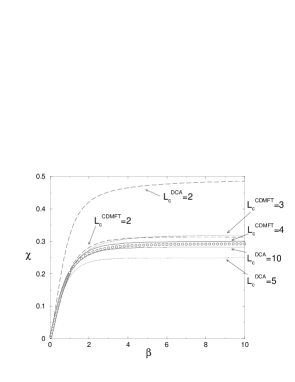
FIG. 1.: $\chi$ as a function of $\beta$ for $\mu=1$, and $t=1$. The points are the exact solution. The lines are $\chi_{cl}^{DCA}$ for $L_{c}=2,5,10$ and $\chi_{cl}^{CDMFT}$ for $L_{c}=2,3,4$.

where $i=1,\dots,L$ and $\sigma=1,\dots,N$ and we take the large $L$ and $N$ limits. In the following we will use $J$ as the unite of temperature and therefore we put $J=1$ and we rescale the hopping term $t\rightarrow t/J$. The thermodynamics of this model can be solved exactly since in the large $N$ limit the quantity $\chi=\frac{1}{N}\sum_{\sigma}f_{i,\sigma}^{\dagger}(t)f_{i+1,\sigma}(t)$ does not fluctuate. Indeed (5) reduces to a free-fermions Hamiltonian with a “renormalized” hopping term $t\rightarrow t+\chi$ and a self-consistent condition on $\chi$:

$$\chi=\frac{1}{L}\sum_{k}f(\beta E_{k})\cos k,\qquad E_{k}=-2(t+\chi)\cos k+\mu$$ (7)

where $\mu$ is the chemical potential, $f(\beta E_{k})$ is the Fermi function and $\beta$ is the inverse temperature.
We now apply the DCA approximation to the Hamiltonian (5). As previously, the computation is simplified by the fact that the quantity $\chi_{cl}^{DCA}=\frac{1}{N}\sum_{\sigma}f_{i,\sigma}^{\dagger}(t)f_{i+1,\sigma}(t)$, where $i$ and $i+1$ belong to the same cluster, does not fluctuate in the large-N limit. As a consequence the functional integral on the cluster degrees of freedom reduce to a simple Gaussian integral. Thus, imposing periodic boundary condition on the cluster, the eq. ${\cal G}^{-1}(k_{c})=G_{c}^{-1}(k_{c})+\Sigma_{c}(k_{c})$ implies: $\Sigma_{c}(k_{c})=2\chi_{cl}^{DCA}\cos k_{c}$. Using the second DCA equation which expresses the cluster Green-function as a function of $\Sigma_{c}(k_{c})$, we obtain the self-consistent DCA relation for $\chi_{cl}^{DCA}$:

$$\chi_{cl}^{DCA} = \frac{1}{L}\sum_{K,k_{c}}f(\beta E_{K,k_{c}})\cos k_{c},$$ (9)

$$\qquad E_{K,k_{c}}=-2t\cos(k_{c}+K)-2\chi_{cl}^{DCA}\cos k_{c}+\mu$$

Note that in the infinite cluster limit one recovers the exact equation (7).

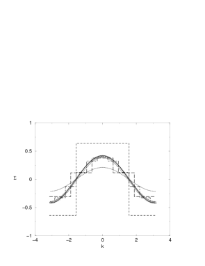
FIG. 2.: Lattice self energy predicted by the different methods compared with the exact solution (triangles) for $t=\beta=\mu=1$. The dotted line is the result of the CDMFT estimator in [6], whereas the continuous line is the result of the first improvement discussed in this paper. The dashed, long dashed and dot dashed lines are respectively the DCA results for $L_{c}=2,5,10$.

Now we focus on the CDMFT approximate solution. As in the DCA case, since the quantity $(\chi_{cl}^{CDMFT})_{i}=\frac{1}{N}\sum_{\sigma}f_{i,\sigma}^{\dagger}(t)f_{i+1,\sigma}(t)$ does not fluctuate, one obtains: $(\Sigma_{c})_{i,j}=(\chi_{cl}^{CDMFT})_{i}\delta_{i,j-1}+(\chi_{cl}^{CDMFT})_{j}\delta_{i,j+1}$. This is the generalization of the corresponding DCA expression to a case without periodic boundary condition. Note that now the quantity $(\chi_{cl}^{CDMFT})_{i}$ may depend on the cluster index. Denoting the eigenvectors and the eigenvalues of the matrix $\hat{t}+\hat{\Sigma}$ respectively $\psi_{i}^{\nu}(K)$ and $\lambda^{\nu}(K)$ ($\nu=1,\dots,L_{c}$), the (ii) CDMFT equation, which expresses the cluster Green-function in terms of the cluster self-energy, reads:

$$(G_{c})_{i,j}=\frac{L_{c}}{L}\sum_{K,\nu}\psi_{i}^{\nu}(K)(\psi_{j}^{\nu}(K))^{*}\frac{1}{i\omega_{n}+\mu-\lambda^{\nu}(K)}$$ (10)

Using this expression we finally get the self-consistent CDMFT equation on $(\chi_{cl}^{CDMFT})_{i}$:

$$(\chi_{cl}^{CDMFT})_{i} = \frac{L_{c}}{L}\sum_{K,\nu}\psi_{i}^{\nu}(K)(\psi_{i+1}^{\nu}(K))^{*}f(\beta E_{K,\nu}),\qquad$$ (12)

$$E_{K,\nu}=\mu-\lambda^{\nu}(K)$$

Notice that eq. 12 corresponds to the exact solution of a model defined by a Hamiltonian similar to (5) in which $J_{i,i+1}$ equals $1$ if $i$ and $i+1$ belong to the same cluster and zero otherwise. This implies in particular that in the infinite cluster limit the CDMFT approximation gives back the exact solution. We have numerically solved the self consistent equations (7,9,12) to compare the DCA and CDMFT predictions for different cluster sizes to the exact solution.

FIG. 3.: $\chi$ as a function of $\beta$ for $\mu=1$, and $t=1.$. The points are the exact solution. The lines are, from top to bottom: $\chi_{cl}^{DCA}$ (dashed line), $\chi_{la}^{DCA}$ (long-dashed line), $\chi_{cl}^{CDMFT}$ (dot-dashed line), $\chi_{la}^{CDMFT2}$ (continuous line), $\chi_{la}^{CDMFT1}$ (dotted line). $\chi_{la}^{CDMFT1}$ is the result obtained using the CDMFT estimator for the lattice self-energy in [6] whereas $\chi_{la}^{CDMFT2}$ corresponds to the first improvement discussed in this paper.

In Fig. (1) we plot the result of this analysis for $t=1,\mu=1$ as a function of $\beta$ and for different cluster sizes. The two methods converge (the convergence is not uniform in $\beta$) toward the exact solution for high enough $L_{c}$ but C-DMFT converges better that DCA. Indeed the C-DMFT result are already surprisingly good for $L_{c}=2$. However, as we shall discuss below, there are two different ways to compute $\chi$ within the cluster methods. The one used here is based on a real space cluster intuition. The second one, relies on a momentum space intuition and computes the correlation functions from the k dependent lattice Greens function, this procedure was advocated in ref [2] and . we will show that it is also gives accurate results for small clusters.

The lattice self-energy. We now address the computation of the lattice self energy. In DCA a discretized form of the lattice self energy in momentum space, enters directly in the evaluation of $G_{0}$. On the other hand, CDMFT focuses on estimating the cluster greens function, and the lattice self energy does not participate in the mean field equations, and has to be estimated later from the cluster self energy. For the simplified large-N one dimensional model studied in this paper the DCA prediction for the lattice self-energy reads:

$$\Sigma_{latt}^{DCA}(k)=\Sigma(k_{c})=2\chi_{cl}^{DCA}\cos k_{c}$$ (13)

where $k$ belongs to $[-\frac{\pi}{L_{c}}+k_{c},k_{c}+\frac{\pi}{L_{c}}]$. Whereas for C-DMFT an estimator for the lattice self energy is constructed using the matrix $S_{R_{n},\alpha;i}=\delta_{R_{n}+\alpha,i}$ where $\alpha$ is the internal cluster index and $i$ denotes a lattice site. The simplest form [6] is: $\Sigma_{latt}^{CDMFT}(k)=\sum_{\alpha,\beta}\tilde{S}^{\dagger}_{\alpha}(k)\Sigma_{\alpha,\beta}\tilde{S}_{\beta}(k)$, where $\tilde{S}_{\alpha}(k)$ is the Fourier transform of the matrix $S$ with respect to the original lattice index $i$. $\tilde{S}_{\alpha}(k)$ can be easily written in terms of the matrix $\hat{U}(k)$ defined before: $\tilde{S}(k)_{\alpha}=U_{\alpha,\alpha}(k)/\sqrt{L_{c}}$. Therefore the relationship between the lattice and the cluster self energy reads: $\Sigma_{latt}^{CDMFT}(k)=\sum_{\alpha,\beta}[U^{\dagger}(k)\Sigma_{c}U(k)]_{\alpha,\beta}/L_{c}$. For example, in the case of the two site cluster we find: $\Sigma_{latt}^{CDMFT}(k)=\chi_{cl}^{CDMFT}cos(k)$, whereas the exact solution gives $\Sigma_{latt}(k)=2\chi_{ex}cos(k)$. As a consequence, even if the value of $\chi$ is well predicted by the CDMFT there is a factor 2 between the two self-energies. The reason of this discrepancy may be understood writing the simple estimator of the lattice self energy [6] in real space $(\Sigma_{latt})_{i-j}=\sum_{\alpha,\beta\,:\,\alpha-\beta=i-j}(\Sigma_{c})_{\alpha,\beta}/L_{c}$. This means that the lattice self energy for a certain value of $i-j$ is obtained averaging over all the cluster self energy elements corresponding to $\alpha-\beta=i-j$. In the limit of an infinite cluster translation invariance implies that the cluster self energy coincides with the lattice self energy in the bulk. Therefore the factor $1/L_{c}$ cancels and we get the exact solution. However for a finite lattice there are only $L_{c}-1$ factors for $i-j=1$, $L_{c}-2$ factors for $i-j$=2 , …$L_{c}-k$ factors for $i-j=k$. Therefore it is highly desirable to have improved estimators for smaller size clusters in which the formula in which the average over all the factors having $\alpha-\beta=k$ is weighted by their number $1/(L_{c}-k)$. One could also think to put an extra weight to extract the lattice self-energy only from the sites in the bulk, for which the CDMFT result should be better. We propose new general class of estimators for the lattice self energy in terms of the cluster self energy, that inherit its causality property.

$$(\Sigma_{latt})_{i-j}=\sum_{\alpha,\beta\,:\,\alpha-\beta=i-j}w_{\alpha,\beta}{(\Sigma_{c})_{\alpha,\beta}}$$ (14)

where the matrix $w_{\alpha,\beta}$ is positive definite and $\sum_{\alpha,\beta\,:\,\alpha-\beta=i-j}w_{\alpha,\beta}\rightarrow 1$ for $L_{c}\rightarrow\infty$ (this guarantees a good behavior in the infinite cluster limit). Using that the trace of the product of two positive definite matrices is positive, one can easily prove that if the cluster self-energy is causal this formula produce a lattice self-energy which is also causal. Note that (14) does not change the behavior for an infinite cluster, but can really improve the results for finite cluster sizes. For example, in Fig. 2 we compare the exact lattice self-energy to the DCA and the CDMFT predictions (using the initial estimator proposed in [6] and the simple improvement $w_{\alpha,\beta}=1/(L_{c}-1)$ which weights in the right way at least the terms with $\alpha-\beta=1$) for $\beta=\mu=t=1$. We remark that there is an excellent agreement between CDMFT and the exact solution after that our simple improvement has been taken into account already for $L_{c}=2$. Whereas the DCA prediction becomes good for $L_{c}\geq 5$.

Relation between lattice and cluster observables. Once the lattice self-energy has been obtained within a cluster method, the lattice Green function can be straightforwardly computed. This offers a different way of estimating the first neighbor correlation function $\chi$, using the lattice Greens function. This quantity can be computed inside the cluster ($\chi_{cl}$) or using the lattice Green function, obtained by the lattice self-energy, ($\chi_{la}$) and the two results do not coincide in general. In the case of C-DMFT one can understand what are the approximations responsible for this difference and why they are small. The C-DMFT approach is based on the cavity procedure [6] which, if it was carried out exactly, it would give back the same answer for the lattice and cluster observables. However, in the approximated cavity procedure adopted in the C-DMFT, one assumes that the contribution to the effective action coming from tracing out all the degrees of freedom outside the cluster is purely gaussian. This is clearly not the case in general and it is the main reason for the non-coincidence of lattice and cluster observables.

In Fig. (3) we compare the DCA and CDMFT predictions for the lattice and cluster values of $\chi$ to the exact solution for a two site cluster, for $t=1,\mu=1$ as a function of $\beta$. These curves display the typical behavior found also for other values of the control parameters: $\chi_{la}^{DCA}$ is quite better than its cluster counterpart, whereas the C-DMFT prediction is quite stable. This is probably the result of having an approximate cavity construction for the C-DMFT [6]. Moreover we remark that $\chi_{la}^{CMDT2}$, obtained using the first improvement for the self-energy discussed above, almost coincides with the exact solution. Comparing the C-DMFT and the DCA lattice values of $\chi$ we note that C-DMFT gives usually a little bit better answer in terms of accuracy and convergence with respect to cluster size. This is perhaps due to the smoothness of the self-energy in the C-DMFT case.

It would be nice to eliminate the cluster self energy altogether from the C-DMFT approach or to use a self energy without discontinuities in DCA, in the spirit of the work of Katsnelson and Lichtenstein [4]. However, we were unable to prove manifest causality of this approach.

In summary, in this short note we compared the performance of the DCA method with that of the cellular DMFT, in a very simple toy model. We have also proposed new estimators for the lattice self energy within CDMFT, which is more efficient. Our study shows that a direct application of CDMFT, i.e. without exploiting the flexibility inherent in the choice of basis in its most general formulation is very efficient in converging to the correct solution already for a two site cluster. Comparing the DCA and the C-DMFT predictions are a little bit better in terms of accuracy and convergence with respect to cluster size. DCA estimates of physical quantities, are most accurately carried out using the lattice Greens function, and not from the real space cluster correlation functions. This is stressed in ref [2], who view DCA as a momentum space method. C-DMFT is not so sensitive to the choice of cluster or lattice estimators, because of the underlying a cavity construction of the derivation [6]. These results are very encouraging, and warrant further applications of these methods to more realistic and difficult problems. Since the most glaring deficiency of the CDMFT method is that it does not attempt to take into account in a direct fashion the translation invariance of the problem, we concentrated on the phase of this model (finite temperatures) which is translationally invariant. We expect that CDMFT will perform even better for the ground state properties since in this case translation invariance is broken by dimerization.

Acknowledgments: This work was supported by the NSF under grant DMR-0096462 and by the Rutgers Center for Materials Theory. GK acknowledges useful discussions with A. Georges, M. Jarrell, H. Krishnamurthy and Sasha Lichtenstein.

REFERENCES

- [1] A. Georges, G. Kotliar, W. Krauth and M. J. Rozenberg, Rev. Mod. Phys. 68 13 (1996).
- [2] C. Huscroft et al., cond-mat/9910226; M. H. Hettler, M. Mukherjee, M. Jarrell and H. R. Krishnamurthy, cond-mat/9903273; T. Maier, M. Jarrell, T. Pruschke, J. Keller, Eur. Phys. J. B 13, 613 (2000); M. H. Hettler et al., Phys, Rev. B 58, R7475 (1998).
- [3] A. Schiller and K. Ingersent, Phys. Rev. Lett. 75, 113 (1995). G. Zarand, D. Cox A. Schiller Phys. Rev. B 62, R16227 (2000).
- [4] A. I. Lichtenstein and M. I. Katsnelson, Phys. Rev. B 62, R9283 (2000).
- [5] I. Affleck and B. Marston, Phys. Rev. B 37, 3774 (1988).
- [6] G. Kotliar, S. Y. Savrasov G. Palsson and G. Biroli Phys. Rev. Lett 87, 186401 (2001). .
- [7] F. Ducastelle, J. Phys. C. Sol. State Phys. 7, 1795 (1974).
- [8] H. Kajueter Rutgers Ph.D thesis (1996) http://www.physics.rutgers.edu/ kotliar/thesis.html Q. Si and J. L. Smith, Phys. Rev. Lett. 77,3391 (1996). J. L. Smith and Q. Si, Phys. Rev. B 61, 5184 (2000).