Scattering theory on graphs

Abstract

We consider the scattering theory for the Schrödinger operator $-{\rm D}_{x}^{2}+V(x)$ on graphs made of one-dimensional wires connected to external leads. We derive two expressions for the scattering matrix on arbitrary graphs. One involves matrices that couple arcs (oriented bonds), the other involves matrices that couple vertices. We discuss a simple way to tune the coupling between the graph and the leads. The efficiency of the formalism is demonstrated on a few known examples.

^(a)Laboratoire de Physique Théorique et Modèles Statistiques. Université Paris-Sud, Bât. 100,
^(b)Laboratoire de Physique des Solides. Université Paris-Sud, Bât. 510, F-91405 Orsay Cedex, France.

E-mail : gilles@lps.u-psud.fr texier@ipno.in2p3.fr, texier@lps.u-psud.fr

PACS : 03.65.Nk, 72.10.Bg, 73.23.-b

1 Introduction

The study of graphs is a vast domain. Spectral theory of the Laplacian on graphs has been widely studied in the mathematical literature [1, 2, 3, 4]. Here we are interested on graphs made of one-dimensional wires identified with finite interval of ${\ensmathonze R}$ and being connected at vertices. A trace formula for the partition function of the Laplace operator on such graphs has been derived in a very nice work by J.-P. Roth [5, 6] who expressed the partition function in terms of contributions of periodic orbits. The study of the Laplace operator on graphs has been shown to be relevant in many physical situations. It has been first considered for the study of organic molecules [7]. It has also some interest in the context of superconducting networks [8], for the study of adiabatic quantum transport in networks [9, 10] and in the weak localization theory [11, 12, 13, 14, 15]. More precisely several physical quantities of weak localization theory are related to the spectral determinant of the Laplace operator $S(\gamma)=\det(-{\rm D}_{x}^{2}+\gamma)$, that can be expressed in terms of the determinant of a $V\times V$ matrix $M$ coupling the vertices [14]. The relation between $S(\gamma)$ and the trace formula obtained by Roth has been examined in [16]. Graphs have also been a subject of several studies in the context of quantum chaos for their spectral properties [17, 18, 19, 20] and also their scattering properties when they are connected to leads [21]. Scattering theory on graphs has been studied in [22] and also frequently used in the context of transport theory for mesoscopic networks (e.g. [23, 24, 25, 26]) ; more recently graphs were considered [27] to describe mesoscopic 2-D normal metal networks and superconducting networks realized experimentally to reveal the so-called Aharonov-Bohm cage effect [28, 29]. In order to describe disordered networks, for example to understand how the Aharonov-Bohm cage effect is affected by disorder, it is important to have a simple and efficient formalism which incorporates a potential on the bonds.

In this work we consider the scattering theory for a graph on the bonds of which lives a potential $V(x)$ and connected to external leads from which some wave is injected. Some spectral properties of the Schrödinger operator on graphs have already been studied in [30]. More recently J. Desbois [31, 32] generalized to the case of the Schrödinger operator the result for the spectral determinant of the Laplace operator by one of us and M. Pascaud [14]. Concerning scattering properties, star graphs with potential on the bonds have been studied in [33]. The aim of our work is to provide a general and systematic framework to construct the scattering matrix of a given graph in terms of matrices encoding the information on the topology and the potential on the graph.

The paper is organized as follows : in the next section we introduce the basic definitions. In section 3 we derive an expression of the scattering matrix of the graph in terms of arc matrices (24). In section 4 we take a different point of view and express the scattering matrix in terms of vertex matrices (43,48). Our results generalize the formulae known for the Schrödinger operator $-{\rm D}_{x}^{2}$ in the absence of scattering by the bonds [10, 18]. We will see that the second formulation of the scattering matrix with vertex matrices offers the advantage of compactness compared to the arc matrix formulation. We discuss, in section 5, simple modifications of the formalism to introduce tunable couplings between the leads and the graph in the most efficient way. Simple examples are developed.

2 Position of the problem

We first define the problem and recall the notations chosen in [16, 31]. We consider the Schrödinger operator

$$H=-{\rm D}_{x}^{2}+V(x)$$ (1)

where ${\rm D}_{x}={\rm d}_{x}-{\rm i}A(x)$ is the covariant derivative and the $x$ coordinate lives on a graph ${\cal G}$ made of $B$ one-dimensional wires connected at $V$ vertices. Throughout this paper we will designate the vertices with greek letters ($\alpha$, $\beta$, $\mu$,…). We introduce the $V\times V$-adjacency matrix $a_{\alpha\beta}$ : if the vertices $\alpha$ and $\beta$ are linked by a bond then $a_{\alpha\beta}=1$ and $a_{\alpha\beta}=0$ otherwise. The coordination of vertex $\alpha$ (number of bonds issuing from the vertex) is $m_{\alpha}=\sum_{\beta}a_{\alpha\beta}$. We call $x_{\alpha\beta}\in[0;l_{\alpha\beta}]$ the coordinate on the bond $({\alpha\beta})$ of length $l_{\alpha\beta}$ (note that by definition $x_{\beta\alpha}=l_{\alpha\beta}-x_{\alpha\beta}$).

The Schrödinger operator acts on scalar functions $\psi(x)$ living on ${\cal G}$ that are represented by a set of $B$ components $\psi_{({\alpha\beta})}(x_{\alpha\beta})$ satisfying appropriate boundary conditions at the vertices [9, 10, 34] :

(i) continuity

$$\psi_{(\alpha\beta_{i})}(x_{\alpha\beta_{i}}=0)=\psi_{\alpha}\ \ \mbox{ for }\ \ i=1,\cdots,m_{\alpha}$$ (2)

The indice $\beta_{i}$ designates a vertex neighbour of vertex $\alpha$ ; the wave function at the vertex is $\psi_{\alpha}$.

(ii) A second condition sufficient to ensure current conservation (i.e. unitarity of the scattering matrix)

$$\sum_{\beta}a_{\alpha\beta}\,{\rm D}_{x_{\alpha\beta}}\psi_{(\alpha\beta)}(x_{\alpha\beta}=0)=\lambda_{\alpha}\psi_{\alpha}\>,$$ (3)

where $\lambda_{\alpha}$ is a real parameter. Due to the presence of the connectivity matrix $a_{\alpha\beta}$, the sum runs over all neighbouring vertices linked with vertex $\alpha$. To have a better understanding of the physical meaning of the parameter $\lambda_{\alpha}$ we remark that for a vertex of coordination number 2 the equation (3) describes a potential $\lambda_{\alpha}\delta(x_{\alpha\beta})$ at the position of the vertex $\alpha$. Note also that the limit $\lambda_{\alpha}\to\infty$ corresponds to Dirichlet condition $\psi_{\alpha}=0$ which means that no current is transmitted through this vertex.

It is also possible to consider more general boundary conditions than (2,3) and release the continuity condition as it was proposed in [22].

The magnetic flux along the bond is denoted by $\theta_{\alpha\beta}=\int_{\alpha}^{\beta}{\rm d}x\,A(x)=-\theta_{\beta\alpha}$.

We also introduce the notion of arc which is an oriented bond. Each bond $({\alpha\beta})$ is associated with two arcs : ${\alpha\beta}$ and ${\beta\alpha}$. Throughout this paper we will label the arcs with roman letters ($i$, $j$,…) and designate the reversed arc of $i$ with a bar : $\bar{i}$.

To describe the potential $V_{({\alpha\beta})}(x_{\alpha\beta})$ on the bond $({\alpha\beta})$ it will be appropriate to introduce reflection and transmission coefficients. We call $r_{\alpha\beta}(E)$ and $t_{\alpha\beta}(E)$ reflection and transmission probability amplitudes associated with the transmission from vertex $\alpha$ to vertex $\beta$ for a plane wave of energy $E$. The scattering $2\times 2$-matrix for the bond is

$$\left(\begin{array}[]{cc}r_{\alpha\beta}&t_{\beta\alpha}\\ t_{\alpha\beta}&r_{\beta\alpha}\end{array}\right)$$ (4)

We are considering a scattering problem, that is we consider a situation where the graph ${\cal G}$ is connected to $L$ external leads by which some wave is injected (see figure 1). The on-shell scattering matrix $\Sigma$ is a $L\times L$-matrix that relates the incoming amplitudes in the $L$ channels to the outcoming ones. We call $A^{\rm ext}_{\alpha}$ (resp. $B^{\rm ext}_{\alpha}$) the incoming (resp. outcoming) amplitude on the external lead connected at the vertex $\alpha$. By definition :

$$B^{\rm ext}=\Sigma\>A^{\rm ext}\>.$$ (5)

The purpose of the paper is to express $\Sigma$ by means of arc $2B\times 2B$-matrices and vertex $V\times V$-matrices. We will generalize the expressions known in the absence of potential [10, 18, 21].

Figure 1: A graph made of $B=15$ internal bonds and $V=11$ vertices connected to $L=4$ external leads.

3 Scattering matrix in terms of arc matrices

In this section we construct the scattering matrix by relating it to arc matrices.

Scattering by bonds

We have already explained in section 2 how to describe the scattering by the potential $V(x)$ on the bonds by $2\times 2$-scattering matrices. We associate to each internal arc $i$ two amplitudes $A^{\rm int}_{i}$ and $B^{\rm int}_{i}$ (see figure 2) ; this means that the component $\psi_{i}(x)$ of the wave function of energy $k^{2}$ matches with $A^{\rm int}_{i}{\mbox{\large e}}^{-{\rm i}kx}+B^{\rm int}_{i}{\mbox{\large e}}^{{\rm i}kx}$ at the node from which arc $i$ issues. It follows that the amplitudes at the two boundaries of the arc $i$ are related by :

$$\left(\begin{array}[]{c}A^{\rm int}_{i}\\ A^{\rm int}_{\bar{i}}\end{array}\right)=\left(\begin{array}[]{cc}r_{i}&t_{\bar{i}}\\ t_{i}&r_{\bar{i}}\end{array}\right)\left(\begin{array}[]{c}B^{\rm int}_{i}\\ B^{\rm int}_{\bar{i}}\end{array}\right)\>,$$ (6)

where $\bar{i}$ is the reversed arc. This relation may be more conveniently written in terms of a matrix $R$ that couples the $2B$ internal arcs :

$$A^{\rm int}_{i}=\sum_{j}R_{ij}B^{\rm int}_{j}$$ (7)

with

$$R_{ij}=r_{i}\delta_{i,j}+t_{\bar{i}}\delta_{\bar{i},j}$$ (8)

where $\delta_{i,j}$ is the Kronecker symbol and indices $i$ and $j$ run over the labels of the $2B$ internal arcs : $i,j\in\{1,\cdots,B,\bar{1},\cdots,\bar{B}\}$.

Figure 2: the amplitudes on the arcs $i$ and $\bar{i}$.

If there is no potential on the bonds ($V(x)=0$) we recover the $R$-matrix introduced in [16] :

$$R^{0}_{ij}={\mbox{\large e}}^{{\rm i}kl_{i}}\delta_{\bar{i},j}\>.$$ (9)

The reflection and transmission coefficients characterize the scattering by the potential alone and if we introduce a magnetic field, the modification brought is straightforward : the transmission amplitudes receive additional phases $t_{i}\to t_{i}{\mbox{\large e}}^{{\rm i}\theta_{i}}$ and the reflection amplitudes are not affected by the magnetic field. $\theta_{{\alpha\beta}}=\int_{\alpha}^{\beta}{\rm d}x\,A(x)=-\theta_{\beta\alpha}$ is the magnetic flux along arc ${\alpha\beta}$. The bond scattering matrix then reads :

$$R_{ij}=r_{i}\delta_{i,j}+t_{\bar{i}}{\mbox{\large e}}^{-{\rm i}\theta_{i}}\delta_{\bar{i},j}$$ (10)

This matrix can also be written in a vertex notation (we identify $i$ with ${\alpha\beta}$ and $j$ with $\mu\nu$) :

$$R_{\alpha\beta,\mu\nu}=a_{\alpha\beta}a_{\mu\nu}\left(r_{\alpha\beta}\delta_{\alpha\mu}\delta_{\beta\nu}+t_{\beta\alpha}{\mbox{\large e}}^{{\rm i}\theta_{\beta\alpha}}\delta_{\alpha\nu}\delta_{\beta\mu}\right)\>,$$ (11)

where the adjacency matrix elements $a_{\alpha\beta}$ and $a_{\mu\nu}$ ensure that $\alpha$ and $\beta$ are connected by a bond, as well as $\mu$ and $\nu$.

Scattering by vertices

The bond scattering matrix only couples amplitudes $A^{\rm int}$ and $B^{\rm int}$ associated with internal arcs. On the other hand some vertices ($L$) couple internal bonds and external leads. We write the wave function on the lead connected to the vertex $\alpha$ as (see figure 1) :

$$\psi_{{\rm lead}\>\alpha}(x)=A^{\rm ext}_{\alpha}{\mbox{\large e}}^{-{\rm i}kx}+B^{\rm ext}_{\alpha}{\mbox{\large e}}^{{\rm i}kx}$$ (12)

($x=0$ coincides with the vertex). Since we have to introduce only one pair of amplitudes $A^{\rm ext}_{\alpha}$, $B^{\rm ext}_{\alpha}$ per external lead, this means that each lead is described by one arc only. Adopting this convention implies that we are now dealing with $2B+L$ arcs. We group the internal and external amplitudes in a unique vector :

$$A=\left(\begin{array}[]{c}A^{\rm int}\\ \hline\cr A^{\rm ext}\end{array}\right)\hskip 14.22636pt\mbox{ and }\hskip 14.22636ptB=\left(\begin{array}[]{c}B^{\rm int}\\ \hline\cr B^{\rm ext}\end{array}\right)\>.$$ (13)

If we consider a given vertex $\alpha$ of coordination $m_{\alpha}$, it follows from (2,3) that the $m_{\alpha}$ incoming amplitudes $A_{i}$ at the vertex are related to the outgoing amplitudes $B_{i}$ by a $m_{\alpha}\times m_{\alpha}$ unitary matrix $Q_{\alpha}$ whose diagonal elements are $\frac{2}{m_{\alpha}+{\rm i}\lambda_{\alpha}/k}-1$, all other being $\frac{2}{m_{\alpha}+{\rm i}\lambda_{\alpha}/k}$. We call $Q$ the $(2B+L)\times(2B+L)$-vertex scattering matrix of the whole graph with leads [16] :

$$B_{i}=\sum_{j}Q_{ij}A_{j}$$ (14)

with :

$$Q_{ij} = \frac{2}{m_{\alpha}+{\rm i}\lambda_{\alpha}/k}-1\hskip 14.22636pt\mbox{ if }i=j\mbox{ ($i$ issues from the vertex $\alpha$)}$$ (15)

$$= \frac{2}{m_{\alpha}+{\rm i}\lambda_{\alpha}/k}\hskip 32.72049pt\mbox{ if }i\neq j\ \mbox{ both issuing from the vertex $\alpha$}$$ (16)

$$= 0\hskip 85.35826pt\mbox{ otherwise}\>.$$ (17)

We can also write the matrix elements for the internal arcs in a vertex notation :

$$Q_{\alpha\beta,\mu\nu}=a_{\alpha\beta}a_{\mu\nu}\delta_{\alpha\mu}\left(\frac{2}{m_{\alpha}+{\rm i}\lambda_{\alpha}/k}-\delta_{\beta\nu}\right)\>.$$ (18)

All the information on the topology of the graph is encoded in the matrix $Q$.

Scattering by the full graph

We have seen that the scattering by bonds relates internal amplitudes :

$$A^{\rm int}=R\>B^{\rm int}$$ (19)

and the scattering by vertices all amplitudes :

$$B=Q\>A\>.$$ (20)

We separate the $Q$ matrix into 4 block matrices :

$$Q=\left(\begin{array}[]{c|c}Q^{\rm int}&\tilde{Q}^{\rm T}\\ \hline\cr\tilde{Q}&Q^{\rm ext}\end{array}\right)$$ (21)

where $Q^{\rm T}$ is the transposed matrix ($Q^{\rm int}$ is a $2B\times 2B$-matrix, $Q^{\rm ext}$ is a $L\times L$-matrix and $\tilde{Q}$ is a $L\times 2B$-matrix). In the following we will always choose to write the matrix $Q$ according to this structure.

Equation (20) becomes :

$$B^{\rm int} = Q^{\rm int}\,A^{\rm int}+\tilde{Q}^{\rm T}\,A^{\rm ext}$$ (22)

$$B^{\rm ext} = \tilde{Q}\,A^{\rm int}+Q^{\rm ext}\,A^{\rm ext}\>.$$ (23)

We can now eliminate in (19,22,23) the internal amplitudes and relate $A^{\rm ext}$ to $B^{\rm ext}$. Therefore we obtain the scattering matrix of the graph :

$$\Sigma=Q^{\rm ext}+\tilde{Q}\,({R^{\dagger}-Q^{\rm int}})^{-1}\,\tilde{Q}^{\rm T}\>.$$ (24)

We have used the unitarity of $R$ :

$$(R^{-1})_{ij}=(R^{\dagger})_{ij}=r_{i}^{*}\delta_{i,j}+t_{i}^{*}{\mbox{\large e}}^{-{\rm i}\theta_{i}}\delta_{\bar{i},j}\>.$$ (25)

The expression (24) generalizes the result known in the absence of potential [21].

Example

As an example we consider the scattering on the ring of perimeter $l$ pierced by a flux $\theta$ (figure 3) without potential. This graph possesses one internal bond (arcs $1$ and $\bar{1}$) ; the external lead is associated with an arc called $1e$. The bond scattering matrix (10,11) is :

$$R=\left(\begin{array}[]{cc}0&{\mbox{\large e}}^{{\rm i}kl-{\rm i}\theta}\\ {\mbox{\large e}}^{{\rm i}kl+{\rm i}\theta}&0\end{array}\right)$$ (26)

and the vertex scattering matrix (15,16,17,18), expressed in a basis of arcs $\{1,\bar{1},1e\}$ (see figure 3) for $\lambda_{\alpha}=0$, reads

$$Q=\left(\begin{array}[]{cc|c}-1/3&2/3&2/3\\ 2/3&-1/3&2/3\\ \hline\cr 2/3&2/3&-1/3\end{array}\right)\>.$$ (27)

Figure 3: Scattering in a ring pierced by a magnetic flux.

Applying (24) we find

$$\Sigma=-\frac{3{\mbox{\large e}}^{{\rm i}kl}-4\cos\theta+{\mbox{\large e}}^{-{\rm i}kl}}{3{\mbox{\large e}}^{-{\rm i}kl}-4\cos\theta+{\mbox{\large e}}^{{\rm i}kl}}\>.$$ (28)

With one lead, the scattering matrix is given by a unique phase : $\Sigma(E)={\mbox{\large e}}^{{\rm i}\delta(E)}$ with

$$\mathop{\mathrm{cotg}}\nolimits\frac{\delta}{2}=\frac{\sin kl}{2(\cos\theta-\cos kl)}\>;$$ (29)

we recover a result obtained by relating in the one channel case the scattering matrix to ratio of spectral determinants [16].

Remark : multichannel wires

We remark that the formulation of the scattering in terms of arc matrices can be generalized for multichannel wires : the matrix elements $Q_{ij}$ and $R_{ij}$ would then become submatrices coupling channels.

Multiple scattering expansion

It is sometimes interesting to expand the quantities of interest in terms of contributions of paths in the graph (we call path an ordered set of arcs). Since the matrices $Q$ and $R$ contain the scattering amplitudes on vertices and bonds, respectively, it is obvious that the expansion of (24) expresses the contributions of paths to the transmission amplitudes from one lead to another :

$$\Sigma=Q^{\rm ext}+\tilde{Q}\,R\,\tilde{Q}^{\rm T}+\tilde{Q}\,RQ^{\rm int}R\,\tilde{Q}^{\rm T}+\cdots+\tilde{Q}\,R(Q^{\rm int}R)^{n}\,\tilde{Q}^{\rm T}+\cdots$$ (30)

The first term is associated with transmission from leads without entering the graph. The term $\tilde{Q}R\tilde{Q}^{\rm T}$ corresponds to paths that contain only one bond of the graph. More generally, the element $(\tilde{Q}R(Q^{\rm int}R)^{n}\tilde{Q}^{\rm T})_{ij}$ is the sum of all amplitudes associated to the paths going from lead $j$ to lead $i$, and made of $n+1$ internal arcs.

4 Scattering matrix in terms of vertex matrices

The approach presented in the previous section has the advantage to consider only scattering matrices for bonds and vertices but presents the disagreement to manipulate rather big matrices ($2B\times 2B$). In this section we follow a different methodology by constructing the stationary scattering states in the graph which leads to deal with vertex matrices ($V\times V$) usually smaller.

For convenience we label the vertices connected to leads with the $L$ first indices : $\alpha=1,\cdots,L$, however the final result will be completely independent of the way the basis of vertices is organized.

We introduce the $L\times V$-matrix $W$ [18] containing the information about the way the graph is connected : $W_{\alpha\beta}=\delta_{\alpha\beta}$ with $\alpha\in\{1,\cdots,L\}$ and $\beta\in\{1,\cdots,V\}$ :

$$W=\left(\begin{array}[]{cccc|ccc}1&0&\cdots&0&0&\cdots&0\\ 0&1&\cdots&0&0&\cdots&0\\ \vdots&\vdots&\ddots&\vdots&\vdots&\ddots&\vdots\\ 0&\cdots&0&1&0&\cdots&0\\ \end{array}\right)$$ (31)

We now turn to the construction of the stationary scattering states $\psi^{(\alpha)}(x)$ of energy $k^{2}$ which describes a plane wave entering the graph from the lead connected at vertex $\alpha$ and being scattered by the graph into all leads. We consider the case without magnetic field since the addition of a magnetic field is straightforward by adding the appropriate phases in the transmission coefficients of the bonds.

On the lead connected to vertex $\mu$, the wave function is :

$$\psi^{(\alpha)}_{{\rm lead}\>\mu}(x)=\delta_{\mu\alpha}{\mbox{\large e}}^{-{\rm i}kx}+\Sigma_{\mu\alpha}{\mbox{\large e}}^{{\rm i}kx}\>,$$ (32)

with $x\in[0;+\infty[$.

To construct the wave function on the internal bond $({\mu\beta})$ of the graph, it is convenient to introduce the two linearly independent solutions $f_{\mu\beta}(x_{\mu\beta})$ and $f_{\beta\mu}(x_{\mu\beta})$ of the differential equation

$$\left(-{\rm d}_{x_{\mu\beta}}^{2}+V_{({\mu\beta})}(x_{\mu\beta})+\gamma\right)f(x_{\mu\beta})=0\>$$ (33)

for $x\in[0,l_{\mu\beta}]$ , satisfying the following boundary conditions at the edges of the interval :

$$\left\{\begin{array}[]{l}f_{\mu\beta}(\mu)=1\\[2.84544pt] f_{\mu\beta}(\beta)=0\end{array}\right.\hskip 14.22636pt\mbox{and}\hskip 14.22636pt\left\{\begin{array}[]{l}f_{\beta\mu}(\mu)=0\\[2.84544pt] f_{\beta\mu}(\beta)=1\end{array}\right.$$ (34)

We follow here the construction of the spectral determinant for the Schrödinger operator in [31]. To lighten the expressions we have introduced the obvious notation $f(\mu)\equiv f(x_{\mu\beta}=0)$ and $f(\beta)\equiv f(x_{\mu\beta}=l_{\mu\beta})$. The spectral parameter is :

$$\gamma=-k^{2}-{\rm i}0^{+}\>.$$ (35)

For example, if $V_{({\mu\beta})}(x)=0$ the two functions are : $f_{\mu\beta}(x_{\mu\beta})=\frac{\mathop{\mathrm{sh}}\nolimits\sqrt{\gamma}(l_{\mu\beta}-x_{\mu\beta})}{\mathop{\mathrm{sh}}\nolimits\sqrt{\gamma}l_{\mu\beta}}$ and $f_{\beta\mu}(x_{\mu\beta})=\frac{\mathop{\mathrm{sh}}\nolimits\sqrt{\gamma}x_{\mu\beta}}{\mathop{\mathrm{sh}}\nolimits\sqrt{\gamma}l_{\mu\beta}}$.

We call $\psi^{(\alpha)}_{\mu}$ the wave function at the vertex $\mu$ when the plane wave is injected at vertex $\alpha$. The solution of the Schrödinger equation (33) on the bond $({\mu\beta})$

$$\psi^{(\alpha)}_{({\mu\beta})}(x_{\mu\beta})=\psi^{(\alpha)}_{\mu}\,f_{\mu\beta}(x_{\mu\beta})+\psi^{(\alpha)}_{\beta}\,f_{\beta\mu}(x_{\mu\beta})$$ (36)

already satisfies the continuity condition (2).

If we impose the condition (2) for the wave function on the lead ($\psi^{(\alpha)}_{{\rm lead}\>\mu}(0)=\psi^{(\alpha)}_{\mu}$) we get :

$$\delta_{\mu\alpha}+\Sigma_{\mu\alpha}=\psi^{(\alpha)}_{\mu}\hskip 14.22636pt\mbox{ for }\mu=1,\cdots,L\>.$$ (37)

The solution $\psi^{(\alpha)}(x)$ must also satisfy the condition (3), that is :

$$\sum_{\beta}a_{\mu\beta}\frac{{\rm d}\psi^{(\alpha)}_{({\mu\beta})}}{{\rm d}x_{\mu\beta}}(\mu)+(W^{\rm T}W)_{\mu\mu}\,\frac{{\rm d}\psi^{(\alpha)}_{{\rm lead}\>\mu}}{{\rm d}x}(\mu)=\lambda_{\mu}\psi^{(\alpha)}_{\mu}\hskip 14.22636pt\mbox{ for }\mu=1,\cdots,V\>.$$ (38)

The $(W^{\rm T}W)_{\mu\mu}$ ensures that this contribution to current from leads vanishes if $\mu$ is an internal vertex. This equation can be rewritten as

$$(W^{\rm T}W)_{\mu\mu}\,\left(\delta_{\mu\alpha}-\Sigma_{\mu\alpha}\right)=\sum_{\beta}M_{{\mu\beta}}\psi^{(\alpha)}_{\beta}\hskip 14.22636pt\mbox{ for }\mu=1,\cdots,V\>,$$ (39)

where $M$ is the matrix appearing in the expression of the spectral determinant[31]

$$M_{\mu\beta}(\gamma)=\frac{1}{\sqrt{\gamma}}\left(\delta_{\mu\beta}\left[\lambda_{\mu}-\sum_{\nu}a_{\mu\nu}\frac{{\rm d}f_{\mu\nu}}{{\rm d}x_{\mu\nu}}(\mu)\right]+a_{\mu\beta}\frac{{\rm d}f_{\mu\beta}}{{\rm d}x_{\mu\beta}}(\beta)\right)\>.$$ (40)

If we consider $\psi^{(\alpha)}_{\mu}$ as the matrix elements $(\mu,\alpha)$ of a $V\times L$ matrix $\Psi$, (37,39) can be rewritten in a matrix form :

$$1+\Sigma = W\Psi$$ (41)

$$W^{\rm T}(1-\Sigma) = M\Psi\>.$$ (42)

We obtain the scattering matrix by eliminating $\Psi$ in (41,42) (with the help of the identity recalled in appendix C). Finally we get :

$$\Sigma=-1+2\,W\left(M+W^{\rm T}W\right)^{-1}W^{\rm T}\>.$$ (43)

The last step is to relate the matrix $M$ to the reflection and transmission coefficients of the bonds. For this purpose we note that we could have chosen a different basis of solutions of equation (33) to construct the stationary state (36) on the bond. In particular we could have chosen the right $\phi_{\beta\mu}(x)$ and left $\phi_{\mu\beta}(x)$ stationary scattering states associated with the potential $V_{({\mu\beta})}(x)$ of the bond solely. If we think at the bond potential $V_{\beta\mu}(x)$ with support $[0,l_{\mu\beta}]$ embedded in an infinite line (${\ensmathonze R}$) these states would be written out of the interval as :

$$\begin{array}[]{lcll}\phi_{\mu\beta}(x)&=&{\mbox{\large e}}^{{\rm i}kx}+r_{\mu\beta}\,{\mbox{\large e}}^{-{\rm i}kx}&\mbox{ for }x\leqslant 0\vspace{0.15cm}\\ &=&t_{\mu\beta}\,{\mbox{\large e}}^{{\rm i}k(x-l_{\mu\beta})}&\mbox{ for }x\geqslant l_{\mu\beta}\vspace{0.15cm}\\ \phi_{\beta\mu}(x)&=&t_{\beta\mu}\,{\mbox{\large e}}^{-{\rm i}kx}&\mbox{ for }x\leqslant 0\vspace{0.15cm}\\ &=&{\mbox{\large e}}^{-{\rm i}k(x-l_{\mu\beta})}+r_{\beta\mu}\,{\mbox{\large e}}^{{\rm i}k(x-l_{\mu\beta})}&\mbox{ for }x\geqslant l_{\mu\beta}\end{array}$$ (44)

It is easy to see that the functions $f_{\mu\beta}(x)$ are related to those stationary scattering states by :

$$f_{\mu\beta}(x_{\mu\beta})=\frac{(1+r_{\beta\mu})\,\phi_{\mu\beta}(x_{\mu\beta})-t_{\mu\beta}\,\phi_{\beta\mu}(x_{\mu\beta})}{(1+r_{\mu\beta})(1+r_{\beta\mu})-t_{\mu\beta}\,t_{\beta\mu}}\>.$$ (45)

Then

$$\frac{{\rm d}f_{\mu\beta}}{{\rm d}x_{\mu\beta}}(\mu)={\rm i}k\frac{(1-r_{\mu\beta})(1+r_{\beta\mu})+t_{\mu\beta}\,t_{\beta\mu}}{(1+r_{\mu\beta})(1+r_{\beta\mu})-t_{\mu\beta}\,t_{\beta\mu}}$$ (46)

and

$$\frac{{\rm d}f_{\mu\beta}}{{\rm d}x_{\mu\beta}}(\beta)={\rm i}k\frac{2\,t_{\mu\beta}}{(1+r_{\mu\beta})(1+r_{\beta\mu})-t_{\mu\beta}\,t_{\beta\mu}}\>.$$ (47)

We can now express the matrix $M$ for $\gamma=-k^{2}-{\rm i}0^{+}$ in terms of bond reflections and transmissions :

$\displaystyle M_{\alpha\beta}$ $\displaystyle=$ $\displaystyle\delta_{\alpha\beta}\left({\rm i}\frac{\lambda_{\alpha}}{k}+\sum_{\mu}a_{\alpha\mu}\frac{(1-r_{\alpha\mu})(1+r_{\mu\alpha})+t_{\alpha\mu}\,t_{\mu\alpha}}{(1+r_{\alpha\mu})(1+r_{\mu\alpha})-t_{\alpha\mu}\,t_{\mu\alpha}}\right)$ (48) $\displaystyle\hskip 28.45274pt-a_{\alpha\beta}\frac{2\,t_{\alpha\beta}}{(1+r_{\alpha\beta})(1+r_{\beta\alpha})-t_{\alpha\beta}\,t_{\beta\alpha}}\>.$

This equation with (43) generalizes the result known in the absence of the potential [10, 18]. In the appendix A we rewrite the matrix $M$ with real parameters replacing the complex reflection and transmission coefficients of the bonds, and in the appendix B we discuss how it is modified if the graph contains loops that we don’t want to describe with several vertices.

We repeat that the addition of a magnetic field implies the substitution : $t_{\alpha\beta}\to t_{\alpha\beta}{\mbox{\large e}}^{{\rm i}\theta_{\alpha\beta}}$, the reflections being unchanged.

Note that if $V(x)=0$ we have $r_{\alpha\beta}=0$ and $t_{\alpha\beta}={\mbox{\large e}}^{{\rm i}kl_{\alpha\beta}+{\rm i}\theta_{\alpha\beta}}$ and we recover the well-known matrix [7, 8, 34] that appears in the search of the eigenvalues of the closed graph (if $\lambda_{\alpha}=0$) :

$$M^{0}_{\alpha\beta}={\rm i}\,\delta_{\alpha\beta}\sum_{\mu}a_{\alpha\mu}\mathop{\mathrm{cotg}}\nolimits kl_{\alpha\mu}-a_{\alpha\beta}\frac{{\rm i}\,{\mbox{\large e}}^{{\rm i}\theta_{\alpha\beta}}}{\sin kl_{\alpha\beta}}\>.$$ (49)

Example

We consider again the case of the ring (figure 3) ; this example has been studied in [10]. The graph can be described with only one vertex to which one loop is attached. In this case the matrix $M$ reduces to a scalar (see [15, 16] and appendix B) :

$$M=2{\rm i}\left(\mathop{\mathrm{cotg}}\nolimits kl-\frac{\cos\theta}{\sin kl}\right)\>;$$ (50)

the matrix $W$ reduces to $1$ and we recover straightforwardly from (43) the result (28) :

$$\Sigma=\frac{{\rm i}\sin kl+2(\cos kl-\cos\theta)}{{\rm i}\sin kl-2(\cos kl-\cos\theta)}\>.$$ (51)

Remark : spectral determinant

Note that the spectral determinant $S(\gamma)=\prod_{n}(E_{n}+\gamma)$ characterizing the spectrum of the isolated graph can also be expressed in terms of the reflection and transmission coefficients by using equations (46,47,48) with the result of J. Desbois [31] :

$$S(\gamma)=\gamma^{V/2}\prod_{({\alpha\beta})}\left(\frac{{\rm d}f_{\beta\alpha}}{{\rm d}x_{\alpha\beta}}(\alpha)\right)^{-1}\det M(\gamma)\>.$$ (52)

5 Tuning the coupling of the graph to the leads

In this section we consider the situation where a graph ${\cal G}$ can be decoupled from the leads at which it is connected by tuning some parameters. A way to proceed is to add a bond with a tunable transmission between each lead and the corresponding vertex to which it is plugged in (figure 5) ; this can be described with the formalism we have presented above in the two previous sections but requires to consider a new graph $\tilde{\cal G}$ with $V+L$ vertices and $B+L$ bonds (if ${\cal G}$ has $V$ vertices, $B$ bonds and $L$ leads). The purpose of this section is to demonstrate that the problem can be reduced, in the sense that we can keep considering the original graph ${\cal G}$ with $V$ vertices and $B$ bonds, provided some modifications of the above formalism are made : (i) in the “arc matrices” formulation we have to modify the vertex scattering matrix for vertices connected to leads. (ii) In the “vertex matrices” formulation, formulae (43,48) still hold using the matrix $M$ of ${\cal G}$ if we modify the matrix $W$ in a way that appears to be very natural.

A vertex scattering matrix including arbitrary coupling of one arc

We construct the scattering matrix of the graph of figure 4 made of one bond (two arcs $0$ and $\bar{0}$). To describe the scattering on the bond $(0)$ we choose a simple bond scattering matrix (10)

$$R=\left(\begin{array}[]{cc}\cos\xi&\sin\xi\\ \sin\xi&-\cos\xi\end{array}\right)$$ (53)

that allows to tune the transmission probability through the bond : $T=\sin^{2}\xi$. At one side of the bond, $m-1$ arcs are connected and only one at the other side. The scattering matrix we will obtain is the scattering matrix for a vertex with $m$ arcs among which one can be disconnected by tuning the parameter $\xi$, all other arcs being equivalent.

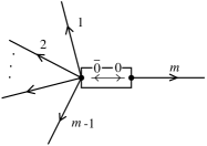
Figure 4: The box on the arc $0$ represents a potential characterized by the scattering matrix (53). The arc $m$ can be decoupled from the other external arcs by tuning the transmission through the bond $(0)$.

In the basis of arcs $\{0,\bar{0},1,2,\cdots,m\}$, the matrix $Q$ (15,16,17) is :

$$Q=\left(\begin{array}[]{cc|ccccc}\frac{2}{m}-1&0&\frac{2}{m}&\frac{2}{m}&\cdots&\frac{2}{m}&0\\ 0&0&0&0&\cdots&0&1\\ \hline\cr\frac{2}{m}&0&\frac{2}{m}-1&\frac{2}{m}&\cdots&\frac{2}{m}&0\\[2.84544pt] \frac{2}{m}&0&\frac{2}{m}&\frac{2}{m}-1&\cdots&\frac{2}{m}&0\\ \vdots&\vdots&\vdots&\vdots&\ddots&\vdots&\vdots\\ \frac{2}{m}&0&\frac{2}{m}&\frac{2}{m}&\cdots&\frac{2}{m}-1&0\\ 0&1&0&0&\cdots&0&0\end{array}\right)\>.$$ (54)

The matrix has been written with the parameter $\lambda=0$ to lighten the expressions. This parameter is straightforwardly re-introduced by performing the following substitution :

$$m\to m+{\rm i}\frac{\lambda}{k}\>.$$ (55)

We now use the equation (24) to express the $m\times m$ scattering matrix of the graph :

$$\Sigma=\left(\begin{array}[]{c|c}\rho&\tau^{\rm T}\\ \hline\cr\tau&\rho^{\prime}\end{array}\right)\>,$$ (56)

where $\rho$ is a $(m-1)\times(m-1)$ matrix, $\tau$ a line vector of dimension $m-1$ and $\rho^{\prime}$ a number :

$$\rho_{ij} = \frac{2}{m}\,\frac{1+\cos\xi}{1+\left(1-\frac{2}{m}\right)\cos\xi}-\delta_{i,j}\>,$$ (57)

$$\tau_{i} = \frac{2}{m}\,\frac{\sin\xi}{1+\left(1-\frac{2}{m}\right)\cos\xi}\>,$$ (58)

$$\rho^{\prime} = -\frac{1-\frac{2}{m}+\cos\xi}{1+\left(1-\frac{2}{m}\right)\cos\xi}\>;$$ (59)

the indices $i,j$ run over the first $m-1$ equivalent arcs.

A more convenient parametrization is obtained by relating $\xi\in]-\pi,\pi]$ to a parameter $w\in{\ensmathonze R}$ :

$$w=\tan(\xi/2)\>.$$ (60)

We emphasize that the parameter $w$ characterizes only the scattering through the bond $(0)$ (figure 4). With this new parameter the scattering matrix takes the simpler form :

$$\rho_{ij} = \frac{2}{m^{\star}}-\delta_{i,j}\>,$$ (61)

$$\tau_{i} = \frac{2\,w}{m^{\star}}\>,$$ (62)

$$\rho^{\prime} = \frac{2\,w^{2}}{m^{\star}}-1\>,$$ (63)

where we have re-introduced the parameter $\lambda$ in

$$m^{\star}=m-1+w^{2}+{\rm i}\frac{\lambda}{k}\>.$$ (64)

$m^{\star}$ plays the role of an effective coordination number. The expressions (61,62,63) generalize the vertex scattering matrix introduced in [5] to the case of tunable couplings to the leads. These transmission coefficients were used to calculate the weigths of the periodic orbits involved in the trace formula [5, 6] and later in [17, 18, 21].

Let us examine several limiting cases to have a better understanding of the role of the parameter $w$ :

$\bullet$ If $w=1$, the matrix $\Sigma$ is the symmetric $m\times m$ scattering matrix for a vertex of coordinence $m$ given by (15,16,17,18). In this case the transmission of the bond $(0)$ is $T=1$.

$\bullet$ If $w=0$, the last arc is decoupled from the others and no current is transmitted to this arc. The scattering between the $m-1$ other arcs, described by the $(m-1)\times(m-1)$ matrix $\rho$, is given by the usual scattering matrix (15,16,17,18) for a coordinence $m-1$.

$\bullet$ If $w=\sqrt{m-1}$ and $\lambda=0$, the scattering matrix coincides with the one introduced by Shapiro [23] up to an inessential change of the sign of $\rho$ (this case corresponds to $\cos\xi=-1+\frac{2}{m}$, i.e. a transmission $T=\frac{4(m-1)}{m^{2}}$).

$\bullet$ If $w=\pm\infty$, all the arcs are decoupled : $\rho_{ij}=-\delta_{i,j}$, $\tau_{i}=0$ and $\rho^{\prime}=1$. From the point of view of the $m-1$ first arcs, this limit is equivalent to $\lambda=\pm\infty$.

Here we have given a generalization of the scattering matrix proposed in [25] for the case of coordination $m=3$ and $\lambda=0$. A generalization to any $m$ of the parametrization of Büttiker et al. is :

$$\Sigma=\left(\begin{array}[]{ccc|c}b&b&\cdots&\sqrt{\epsilon}\\ b&b&\cdots&\sqrt{\epsilon}\\ \vdots&\vdots&\ddots&\vdots\\ \hline\cr\sqrt{\epsilon}&\sqrt{\epsilon}&\cdots&c\end{array}\right)-1\>,$$ (65)

where $b=\frac{1}{m-1}\left(1+\sqrt{1-(m-1)\epsilon}\right)$ and $c=2-(m-1)b=1-\sqrt{1-(m-1)\epsilon}$. The relation with our parametrization with $w$ is given by : $\sqrt{\epsilon}=\frac{2w}{m^{\star}}$ (then $b=\frac{2}{m^{\star}}$), valid for $\lambda=0$. Note however that the parametrization with $\epsilon\in[0,1/(m-1)]$ does not allow to cover the full range of the parameter $w\in{\ensmathonze R}$, but only the interval $w\in[0,\sqrt{m-1}]$.

Scattering matrix of the graph with arbitrary coupling to the leads

We now consider the graph ${\cal G}$ of figure 5. Each external lead is connected to vertices $\alpha\in\{1,2,\cdots,L\}$ of the graph through a barrier which is described by a parameter $w_{\alpha}\in{\ensmathonze R}$ ; we call those vertices “external vertices”. The scattering matrix of the full graph can be constructed with (24). Let us discuss the structure of the vertex scattering matrix. $Q$ couples arcs issuing from the same vertex ; to help the discussion, let us imagine for a moment that the basis of arcs is organized so that the arcs issuing from the same vertex are grouped. The matrix $Q$ is a block diagonal matrix in such a basis. As above we call $Q_{\alpha}$ the $m_{\alpha}\times m_{\alpha}$ block coupling the arcs issuing from the vertex $\alpha$. The blocks related to internal vertices $\alpha\in\{L+1,\cdots,V\}$ are unchanged, still given by (15,16,17), whereas the blocks coupling arcs issuing from external vertices $\alpha\in\{1,\cdots,L\}$ are now given by (56,61,62,63) :

$$Q_{\alpha}=\frac{2}{m_{\alpha}^{\star}}\left(\begin{array}[]{cccc|c}1&1&\cdots&1&w_{\alpha}\\ 1&1&\cdots&1&w_{\alpha}\\ \vdots&\vdots&\ddots&\vdots&\vdots\\ 1&1&\cdots&1&w_{\alpha}\\ \hline\cr w_{\alpha}&w_{\alpha}&\cdots&w_{\alpha}&w_{\alpha}^{2}\end{array}\right)-1\>,$$ (66)

where $m_{\alpha}^{\star}\equiv m_{\alpha}-1+w_{\alpha}^{2}+{\rm i}\lambda_{\alpha}/k$. The introduction of the couplings in this way does not increase the size of the matrices we have to deal with by using (24).

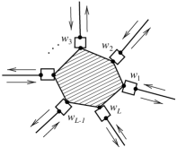
Figure 5: Graph with arbitrary coupling to leads. The couplings $w_{\alpha}$’s are represented by boxes ; we recall that they are defined by $w_{\alpha}=\tan(\xi_{\alpha}/2)$ where the transmission through the box is $T_{\alpha}=\sin^{2}\xi_{\alpha}$. The dashed area schematizes the internal structure of the graph.

We would like now to generalize formula (43) without increasing the difficulty of the calculation of $\Sigma$. The construction of the scattering matrix $\Sigma$ using vertex matrices has used as a basic ingredient the continuity of the wave function at the vertices. If we now describe the scattering at the external vertices with (66), this means that the wave function is not anymore continous at those vertices due to their internal structure (but still continuous at vertices inside the graph). For a moment we focus on the vertex $\alpha$ with $m_{\alpha}$ arcs among which $m_{\alpha}-1$ are internal arcs of the graph, the remaining arc being a lead. We call $A_{1},A_{2},\cdots,A_{m_{\alpha}-1}$ the $m_{\alpha}-1$ incoming amplitudes from the graph and $A_{m_{\alpha}}$ the incoming amplitude from the lead. Let us examine the value of the wave function on the arcs $i$ : $\psi_{i}(x)=A_{i}{\mbox{\large e}}^{-{\rm i}kx}+B_{i}{\mbox{\large e}}^{{\rm i}kx}$. We have $B_{i}=\sum_{j=1}^{m_{\alpha}}(Q_{\alpha})_{ij}A_{j}$ ; on the arc $i$, if $x\to 0$ the wave function goes to $\psi_{i}(0)=A_{i}+B_{i}$. It follows from the expression (66) that we still have the continuity for the wave function on the arcs inside the graph

$$\psi_{1}(0)=\cdots=\psi_{m_{\alpha}-1}(0)=\frac{2}{m_{\alpha}^{\star}}\>{\cal A}+\frac{2\,w_{\alpha}}{m_{\alpha}^{\star}}\>{\cal A^{\prime}}$$ (67)

and the wave function at the extremity of the lead is

$$\psi_{m_{\alpha}}(0)=\frac{2\,w_{\alpha}}{m_{\alpha}^{\star}}\>{\cal A}+\frac{2\,w_{\alpha}^{2}}{m_{\alpha}^{\star}}\>{\cal A^{\prime}}\>,$$ (68)

where ${\cal A}=A_{1}+\cdots+A_{m_{\alpha}-1}$ and ${\cal A^{\prime}}=A_{m_{\alpha}}$. It is straightforward to see that the matrix involved in the two equations has an eigenvalue zero associated with the eigenvector $(w_{\alpha},-1)$. It follows that :

$$\psi_{1}(0)=\cdots=\psi_{m_{\alpha}-1}(0)=\frac{1}{w_{\alpha}}\,\psi_{m_{\alpha}}(0)\>.$$ (69)

This equation replaces the continuity condition for the vertices coupled to the leads.

We now consider the full graph and follow the same lines as in the previous section to construct the scattering matrix, by constructing the stationary scattering state $\psi^{(\alpha)}(x)$ of energy $E=k^{2}$ corresponding to a plane wave injected from the lead $\alpha$. The wave function on the lead connected to the vertex $\mu$ is (32), and (36) on the internal bonds. By virtue of (69) the continuity condition (37) is now replaced by

$$\delta_{\mu\alpha}+\Sigma_{\mu\alpha}=w_{\mu}\>\psi^{(\alpha)}_{\mu}\hskip 14.22636pt\mbox{ for }\mu=1,\cdots,L\>.$$ (70)

The current conservation reads :

$${\psi_{\mu}^{(\alpha)}}^{*}\sum_{\beta}a_{\mu\beta}\,{\rm d}_{x}\psi^{(\alpha)}_{({\mu\beta})}(\mu)+{\psi^{(\alpha)*}_{{\rm lead}\>\mu}}(\mu)\,{\rm d}_{x}\psi^{(\alpha)}_{{\rm lead}\>\mu}(\mu) = \lambda_{\mu}\big{|}\psi_{\mu}^{(\alpha)}\big{|}^{2}\hskip 14.22636pt\mbox{ for }\mu=1,\cdots,L$$ (71)

$$\sum_{\beta}a_{\mu\beta}\,{\rm d}_{x}\psi^{(\alpha)}_{({\mu\beta})}(\mu) = \lambda_{\mu}\psi_{\mu}^{(\alpha)}\hskip 14.22636pt\mbox{ for }\mu=L+1,\cdots,V$$ (72)

that is now rewritten

$$w_{\mu}\,\left(\delta_{\mu\alpha}-\Sigma_{\mu\alpha}\right) = \sum_{\beta}M_{{\mu\beta}}\psi^{(\alpha)}_{\beta}\hskip 14.22636pt\mbox{ for }\mu=1,\cdots,L$$ (73)

$$0 = \sum_{\beta}M_{{\mu\beta}}\psi^{(\alpha)}_{\beta}\hskip 14.22636pt\mbox{ for }\mu=L+1,\cdots,V\>.$$ (74)

Equations (70,73,74) have the same form as (41,42) provided the $L\times V$ matrix $W$ is now defined as :

$$W_{\alpha\beta}=w_{\alpha}\>\delta_{\alpha\beta}\>,$$ (75)

with $w_{\alpha}\in{\ensmathonze R}$. The introduction of tunable couplings between the graph and the leads in (43,48) is thus a simple modification of the matrix $W$ with (75).

Resonances

It is easy to see from the above formalism how the spectrum of resonances of the graph connected to external leads is related to the eigenvalues spectrum of the same isolated graph. The spectrum of resonances is given by the poles of the scattering matrix, the real part of the pole being the energy of the resonance and the imaginary part its width.

(i) In the vertex matrix formulation, the poles of $\Sigma$ are the complex zeros of $\det(M+W^{\rm T}W)$. The matrix $M$ encodes all the information on the isolated graph (topology of the graph and potential on the bonds) whereas the information on the way the graph is coupled to the external leads is contained in $W$. If we turn off the couplings $w_{\alpha}\to 0$, it is clear that we recover the energies of the isolated graph, solutions of $\det M(-k^{2})=0$ (see [31] and remark of section 4).

(ii) In the arc matrix formulation, the poles are the zeros of $\det(1-RQ^{\rm int})$. Now the informations on the topology of the graph and the couplings are mixed in $Q^{\rm int}$ whereas $R$ encodes the information on the potential. Again, if the couplings are switched off, the matrix $Q^{\rm int}$ is equal to the matrix $Q$ of the isolated graph whose spectrum is given by $\det(1-RQ)=0$.

Example 1

We compute the scattering matrix of a ring connected to one lead (figure 6). This is the situation considered in [26]. The result is obtained by replacing (27) by (66) in the calculation we have already done. A more direct way is to use (43,75), $\Sigma=-1+2\frac{w^{2}}{M+w^{2}}$, the matrix $M$ being given by (50).

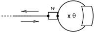
Figure 6: Ring with arbitrary coupling $w$ to the lead.

If we consider the case of a ring with a potential on the bond like in figure 6, $M$ is given by $M=2{\rm i}\frac{\cos\Phi-\sqrt{T}\cos\theta}{\sin\Phi-\sqrt{1-T}\cos\varphi}$, as explained in appendix B. We obtain $\Sigma={\mbox{\large e}}^{{\rm i}\delta}$ with :

$$\mathop{\mathrm{cotg}}\nolimits\frac{\delta}{2}=w^{2}\,\frac{\sin\Phi-\sqrt{1-T}\cos\varphi}{2(\sqrt{T}\cos\theta-\cos\Phi)}\>.$$ (76)

For $w=0$ the ring is disconnected from the arm and the phase shift is constant ($\delta=\pi$). We now consider the case without a potential on the ring : $T=1$, $\Phi=kl$.

$$\mathop{\mathrm{cotg}}\nolimits\frac{\delta}{2}=w^{2}\,\frac{\sin kl}{2(\cos\theta-\cos kl)}\>.$$ (77)

If $w=1$ we recover the result (29). The effect of the parameter $w$ can be seen clearly if we compute $\frac{{\rm d}\delta}{{\rm d}k}$ (see figure 7) :

$$\frac{{\rm d}\delta}{{\rm d}k}=l\,w^{2}\frac{1-\cos\theta\cos kl}{(\cos\theta-\cos kl)^{2}+\frac{1}{4}w^{4}\sin^{2}kl}\>.$$ (78)

We now discuss the two ways to decouple the lead from the ring.

$\bullet$ In the limit $w\to 0$, the width of the resonance peaks is $\Delta k=\frac{w^{2}}{2\,l}$, the peaks being centered on the eigen-energies of the isolated ring of perimeter $l$ : $k_{n}^{\pm}l=\pm\theta+2n\pi$, with $n\in{\ensmathonze N}$ for the sign $+$ and $n\in{\ensmathonze N}^{*}$ for the sign $-$. We have : $\frac{{\rm d}\delta}{{\rm d}k}\simeq 2\pi\frac{\Delta k/\pi}{(k-k_{n}^{\pm})^{2}+\Delta k^{2}}$ if $k\sim k_{n}^{\pm}$.

$\bullet$ In the limit $w\to\infty$ the three arcs decouple, the ring is open, and $\frac{{\rm d}\delta}{{\rm d}k}$ presents peaks of width $\Delta\kappa=\frac{2}{w^{2}l}(1-(-1)^{m}\cos\theta)$ centered on the eigen-energies of the isolated line of length $l$ : $\kappa_{m}l=m\pi$, for $m\in{\ensmathonze N}$.

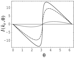
Figure 7: Left : $\frac{{\rm d}\delta}{{\rm d}k}$ for the ring of figure 6 for different values of the coupling $w$. Dotted lines : $w=1$, dashed lines : $w=0.5$ and full lines : $w=0.05$. The flux is $\theta=5\pi/7$ and the length $l=1$. Right : Persistent current $I(k_{F},\theta)=\int_{0}^{k_{F}}{\rm d}k\,2k\,j(k^{2},\theta)$ for $w=0.5$ (full line), $w=1$ (dashed lines) and $w=5$ (dotted lines). We have chosen $k_{F}l=3\pi$.

The physical difference of the two limits may also be seen on the persistent current [35] (see also [36]) : $j(k^{2},\theta)=\frac{1}{2\pi}\frac{\partial}{\partial\theta}\delta(k^{2},\theta)$ is the current density, i.e. $j(E,\theta)\,{\rm d}E$ is the current of the states in the energy range $[E,E+{\rm d}E[$. We get

$$j(k^{2},\theta)=-\frac{1}{2\pi l}\,\frac{\sin\theta\sin kl}{1-\cos\theta\cos kl}\,\frac{{\rm d}\delta}{{\rm d}k}\>.$$ (79)

$\bullet$ If $w\to 0$, the current density presents sharp peaks of alternate signs at the position of the resonances : $j(k^{2},\theta)\simeq\mp\frac{1}{2\pi l}\frac{{\rm d}\delta}{{\rm d}k}$ for $k\sim k^{\pm}_{n}$. We define the contribution of the peak at $k^{\pm}_{n}$ as $I_{n}^{\pm}=\int_{k^{\pm}_{n}-\delta K}^{k^{\pm}_{n}+\delta K}{\rm d}k\,2k\,j(k^{2},\theta)$ with $\delta K$ being a quantity large compare to the resonance width but small compare the distance between peaks : $w^{2}\ll\delta K\,l\ll\mathop{\mathrm{min}}\nolimits\left(\theta,\pi-\theta\right)$. We immediatly see that $I_{n}^{\pm}\simeq\frac{4\pi}{l^{2}}\left(\mp n-\frac{\theta}{2\pi}\right)$ ; we have recovered the persistent current of the isolated ring ${\cal I}_{n}^{\pm}=-\frac{\partial}{\partial\theta}(k_{n}^{\pm})^{2}$.

$\bullet$ In the limit $w\to\infty$, the current density behaves like : $j(k^{2},\theta)\propto(k-\kappa_{m})\frac{{\rm d}\delta}{{\rm d}k}$ in the neighbourhood of the resonance $k\sim\kappa_{m}$. It follows that the contributions of the resonance peaks vanish (due to the opening of the ring) : $I_{m}=\int_{\kappa_{m}-\delta K}^{\kappa_{m}+\delta K}{\rm d}k\,2k\,j(k^{2},\theta)\simeq 0$ (the right part of figure 7 indeed shows that the persistent current decreases as $w$ is increased).

Example 2

We consider a ring pierced by a flux $\theta$ and connected to two leads (see figure 8). This arrangement has been considered in several works to study the Aharonov-Bohm oscillations of the conductance of a normal metal ring : the authors of [24] considered a particular coupling of the leads whereas [25] examined more general couplings.

The ring is made of two arcs $a$ and $b$. We use the parameters of appendix A to write the matrix $M$. Using (89) the matrix $M$ is given by :

$$M_{11} = {\rm i}\frac{\lambda_{1}}{k}+{\rm i}\,\frac{\cos\Phi_{a}+\sqrt{1-T_{a}}\sin\varphi_{a}}{\sin\Phi_{a}-\sqrt{1-T_{a}}\cos\varphi_{a}}+{\rm i}\,\frac{\cos\Phi_{b}+\sqrt{1-T_{b}}\sin\varphi_{b}}{\sin\Phi_{b}-\sqrt{1-T_{b}}\cos\varphi_{b}}$$ (80)

$$M_{21}(\theta) = -\frac{{\rm i}\,\sqrt{T_{a}}\,{\mbox{\large e}}^{{\rm i}\theta/2}}{\sin\Phi_{a}-\sqrt{1-T_{a}}\cos\varphi_{a}}-\frac{{\rm i}\,\sqrt{T_{b}}\,{\mbox{\large e}}^{-{\rm i}\theta/2}}{\sin\Phi_{b}-\sqrt{1-T_{b}}\cos\varphi_{b}}$$ (81)

$$M_{12}(\theta) = M_{21}(-\theta)$$ (82)

$$M_{22} = {\rm i}\frac{\lambda_{2}}{k}+{\rm i}\,\frac{\cos\Phi_{a}-\sqrt{1-T_{a}}\sin\varphi_{a}}{\sin\Phi_{a}-\sqrt{1-T_{a}}\cos\varphi_{a}}+{\rm i}\,\frac{\cos\Phi_{b}-\sqrt{1-T_{b}}\sin\varphi_{b}}{\sin\Phi_{b}-\sqrt{1-T_{b}}\cos\varphi_{b}}\>.$$ (83)

When several bonds link two vertices $\alpha$ and $\beta$, we have to sum the contributions of each bond in $M_{\alpha\alpha}$ and $M_{\alpha\beta}$ (see [15] and appendix C of [16]). Since the two vertices are connected to leads, the matrix $W$ is the $2\times 2$ diagonal matrix : $W={\rm diag}(w_{1},w_{2})$. We can get the scattering matrix from (43) :

$$\Sigma=-1+\frac{2}{\det(M+W^{2})}\left(\begin{array}[]{cc}w_{1}^{2}M_{22}+w_{1}^{2}w_{2}^{2}&-w_{1}w_{2}M_{12}\\ -w_{1}w_{2}M_{21}&w_{2}^{2}M_{11}+w_{1}^{2}w_{2}^{2}\end{array}\right)\>.$$ (84)

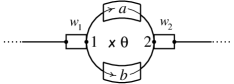
Figure 8: Ring pierced by a magnetic flux $\theta$ with potentials on the bonds.

Now we concentrate ourselves on the case of perfect transmissions through the bonds : $T_{a,b}=1$ and $\Phi_{a,b}=kl_{a,b}$, with $\lambda_{1,2}=0$. We have

$$\det(M+W^{2})=-\frac{2(\cos kl-\cos\theta)}{\sin kl_{a}\sin kl_{b}}+{\rm i}(w_{1}^{2}+w_{2}^{2})\frac{\sin kl}{\sin kl_{a}\sin kl_{b}}+w_{1}^{2}w_{2}^{2}$$ (85)

where $l=l_{a}+l_{b}$ is the perimeter of the ring. If we consider the limit of weak coupling $w_{1,2}\to 0$ we can expand the scattering matrix in the neighbourhood of the eigen-energies of the ring. We obtain the well-known Breit-Wigner form :

$$\Sigma_{{\alpha\beta}}{{\raisebox{-8.5359pt}{$\textstyle\simeq$}}\atop{\scriptstyle{k\sim k_{n}^{\pm}}}}-\delta_{\alpha\beta}+\frac{{\rm i}\sqrt{\Delta k_{\alpha}\Delta k_{\beta}}\,{\mbox{\large e}}^{{\rm i}\chi_{\alpha\beta}}}{k-k_{n}^{\pm}+\frac{{\rm i}}{2}(\Delta k_{1}+\Delta k_{2})}\>,$$ (86)

where $\Delta k_{1,2}=\frac{w_{1,2}^{2}}{l}$, $\chi_{11}=\chi_{22}=0$ and $\chi_{12}=-\chi_{21}=n\pi\pm\frac{1}{2}k_{n}^{\pm}(l_{a}-l_{b})$. Note that a detailed analysis of the resonance structure of the transmission probability through the ring has already been done in [25].

6 Summary

We have given systematic procedures to construct the scattering matrix of graphs made of one-dimensional wires on which lives a potential, and connected to external leads.

In a first approach we used as basic ingredients a scattering matrix (10) describing scattering by the potentials on the bonds and a scattering matrix (15,16,17) providing information on the scattering by vertices and coupling to the external leads. This approach is quite natural in the sense that we combine the scattering matrices of parts of the system to construct the whole scattering matrix (24), however it can become cumbersome since we have to deal with rather big matrices.

A way to reduce the problem is to reformulate it in terms of vertex matrices, which is possible if the scattering at vertices describes wave functions continuous at the vertices, which allows to deal with vertex variables instead of arc variables.

We have described an efficient way to introduce some tunable couplings between the leads and the graph (75), which permits to go continuously from a connected graph to an isolate graph.

We have generalized the results known in the absence of potential [10, 18, 21] by adding scattering on bonds and allowing to tune the couplings to the external leads.

Appendix A Reformulating the matrix $M$

We would like here to use some relations between reflection and transmission coefficients on a bond to rewrite the result (48) in terms of parameters whose physical meanings are more clear. In the core of the paper we have considered that the reflection and transmission coefficients describe the effect of the scalar potential $V(x)$ only. In this appendix we adopt another point of view and consider that these coefficients describe the effect of both the scalar potential $V(x)$ and the vector potential $A(x)$.

Due to the unitarity of the scattering matrix for a given bond $({\alpha\beta})$, it follows that the 4 complex parameters describing the left ($r_{\alpha\beta}$ and $t_{\alpha\beta}$) and right ($r_{\beta\alpha}$ and $t_{\beta\alpha}$) scattering can be parametrized in terms of 4 real parameters :

$$\left(\begin{array}[]{cc}r_{\alpha\beta}&t_{\beta\alpha}\\ t_{\alpha\beta}&r_{\beta\alpha}\end{array}\right)={\mbox{\large e}}^{{\rm i}\Phi_{\alpha\beta}}\left(\begin{array}[]{cc}{\rm i}{\mbox{\large e}}^{{\rm i}\varphi_{\alpha\beta}}\sqrt{1-T_{\alpha\beta}}&{\mbox{\large e}}^{-{\rm i}\chi_{\alpha\beta}}\sqrt{T_{\alpha\beta}}\\[2.84544pt] {\mbox{\large e}}^{{\rm i}\chi_{\alpha\beta}}\sqrt{T_{\alpha\beta}}&{\rm i}{\mbox{\large e}}^{-{\rm i}\varphi_{\alpha\beta}}\sqrt{1-T_{\alpha\beta}}\end{array}\right)\>.$$ (87)

$\Phi_{\alpha\beta}$ is a global phase. $T_{\alpha\beta}\in[0,1]$ is the transmission probability through the barrier. In the absence of a magnetic field, we know that the scattering matrix is symmetric (it is well known that the symmetry of the scattering matrix in the presence of a magnetic field ${\cal B}$ is $\Sigma(-{\cal B})=\Sigma({\cal B})^{\rm T}$) ; it follows that we can identify the asymmetric part of the phase of the transmission coefficients with the magnetic flux

$$\chi_{\alpha\beta}=\theta_{\alpha\beta}\>.$$ (88)

The last phase $\varphi_{\alpha\beta}$ is related to the asymmetry of the potential (for $V_{({\alpha\beta})}(x)=V_{({\alpha\beta})}(l_{\alpha\beta}-x)$ we have $r_{\alpha\beta}=r_{\beta\alpha}$ i.e. $\varphi_{\alpha\beta}=0$ or $\pi$).

Due to these definitions we have the following obvious relations : $T_{\alpha\beta}=T_{\beta\alpha}$, $\Phi_{\alpha\beta}=\Phi_{\beta\alpha}$, $\varphi_{\alpha\beta}=-\varphi_{\beta\alpha}$ and we recall that $\theta_{\alpha\beta}=-\theta_{\beta\alpha}$.

We can now rewrite (48) in terms of these parameters :

$\displaystyle M_{\alpha\beta}$ $\displaystyle=$ $\displaystyle{\rm i}\,\delta_{\alpha\beta}\left(\frac{\lambda_{\alpha}}{k}+\sum_{\mu}a_{\alpha\mu}\frac{\cos\Phi_{\alpha\mu}+\sqrt{1-T_{\alpha\mu}}\sin\varphi_{\alpha\mu}}{\sin\Phi_{\alpha\mu}-\sqrt{1-T_{\alpha\mu}}\cos\varphi_{\alpha\mu}}\right)$ (89) $\displaystyle\hskip 28.45274pt-{\rm i}\,a_{\alpha\beta}\frac{\sqrt{T_{\alpha\beta}}\,{\mbox{\large e}}^{{\rm i}\theta_{\alpha\beta}}}{\sin\Phi_{\alpha\beta}-\sqrt{1-T_{\alpha\beta}}\cos\varphi_{\alpha\beta}}\>.$

As a by-product, it shows that the matrix $M$ is anti-Hermitian : $M^{\dagger}=-M$. To end this appendix, we note that if the potential on the bond vanishes $V_{({\alpha\beta})}(x)=0$, then $T_{\alpha\beta}=1$ and $\Phi_{\alpha\beta}=kl_{\alpha\beta}$.

Appendix B Matrix $M$ for a graph with loops

We explain in this appendix how the matrix $M$ is modified when we want to describe with the minimum number of vertices a graph possessing loops. We consider a graph with a loop threatened by a flux $\theta_{a}$ at the vertex $\alpha$ (see figure 9). The potential on the arc $a$ of the loop is described by four reflection and transmission coefficients : $r_{a}$, $t_{a}$ for the arc $a$ and $r_{\bar{a}}$, $t_{\bar{a}}$ for the reversed arc $\bar{a}$.

Figure 9: A loop at the vertex $\alpha$.

If we follow the lines of section 4 we can see that only the diagonal part of the matrix $M$ (48) is affected by the loops :

$$M_{\alpha\beta}\to M_{\alpha\beta}+\delta_{\alpha\beta}\,M^{\rm loop}_{\alpha\alpha}\>,$$ (90)

where the contribution of the loop is :

$$M^{\rm loop}_{\alpha\alpha} = \frac{(1-r_{a})(1+r_{\bar{a}})+t_{a}t_{\bar{a}}}{(1+r_{a})(1+r_{\bar{a}})-t_{a}t_{\bar{a}}}-\frac{2\,t_{a}}{(1+r_{a})(1+r_{\bar{a}})-t_{a}t_{\bar{a}}}$$ (91)

$$+ \frac{(1+r_{a})(1-r_{\bar{a}})+t_{a}t_{\bar{a}}}{(1+r_{a})(1+r_{\bar{a}})-t_{a}t_{\bar{a}}}-\frac{2\,t_{\bar{a}}}{(1+r_{a})(1+r_{\bar{a}})-t_{a}t_{\bar{a}}}\>.$$

This result is rather natural : $M_{\alpha\alpha}$ receives two contributions from each arc $a$ and $\bar{a}$ of the kind present in the diagonal elements of (48) and since the arc comes back to the same vertex we get also two contributions of the kind present in the off-diagonal elements of (48). After simplification we obtain :

$$M^{\rm loop}_{\alpha\alpha}=2\frac{1-r_{a}r_{\bar{a}}+t_{a}t_{\bar{a}}-t_{a}-t_{\bar{a}}}{(1+r_{a})(1+r_{\bar{a}})-t_{a}t_{\bar{a}}}\>.$$ (92)

We can also express this contribution with the real parameters introduced in the appendix A to describe the scattering by the arc $a$ : $\Phi_{a}=\Phi_{\bar{a}}$, $T_{a}=T_{\bar{a}}$, $\varphi_{a}=-\varphi_{\bar{a}}$ and $\theta_{a}=-\theta_{\bar{a}}$. We obtain :

$$M^{\rm loop}_{\alpha\alpha}=2{\rm i}\frac{\cos\Phi_{a}-\sqrt{T_{a}}\cos\theta_{a}}{\sin\Phi_{a}-\sqrt{1-T_{a}}\cos\varphi_{a}}\>.$$ (93)

Appendix C Inversion of block matrices

We recall in this appendix a result that can be found in standard textbooks. Consider the square matrix

$${\cal M}=\left(\begin{array}[]{c|c}A&B\\ \hline\cr C&D\end{array}\right)$$ (94)

where $A$ and $D$ are square matrices of arbitrary dimensions. Then :

$${\cal M}^{-1} = \left(\begin{array}[]{c|c}(A-BD^{-1}C)^{-1}&-(A-BD^{-1}C)^{-1}BD^{-1}\\ \hline\cr-D^{-1}C(A-BD^{-1}C)^{-1}&D^{-1}+D^{-1}C(A-BD^{-1}C)^{-1}BD^{-1}\end{array}\right)$$ (97)

$$= \left(\begin{array}[]{c|c}A^{-1}+A^{-1}B(D-CA^{-1}B)^{-1}CA^{-1}&-A^{-1}B(D-CA^{-1}B)^{-1}\\ \hline\cr-(D-CA^{-1}B)^{-1}CA^{-1}&(D-CA^{-1}B)^{-1}\end{array}\right)\>.$$ (100)

References

- [1] N. Biggs, Algebraic Graph Theory, Cambridge University Press, 1976.
- [2] F. Chung, Spectral Graph Theory, American Mathematical Society, 1997.
- [3] Y. Colin de Verdière, Spectres de Graphes, Société Mathématique de France, 1998.
- [4] D. M. Cvetkovic, M. Doob, and H. Sachs, Spectra of graphs, Theory and Application, Academic Press, 1980.
- [5] J.-P. Roth, Spectre du Laplacien sur un graphe, C. R. Acad. Sc. Paris 296, 793 (1983).
- [6] J.-P. Roth, Le spectre du Laplacien sur un graphe, in Colloque de Théorie du potentiel - Jacques Deny, page 521, Orsay, 1983.
- [7] K. Rudenberg and C. Scherr, J. Chem. Phys. 21, 1565 (1953).
- [8] S. Alexander, Superconductivity of networks. A percolation approach to the effects of disorder, Phys. Rev. B 27(3), 1541 (1983).
- [9] J. E. Avron, A. Raveh, and B. Zur, Adiabatic quantum transport in multiply connected systems, Rev. Mod. Phys. 60, 873 (1988).
- [10] J. E. Avron and L. Sadun, Adiabatic quantum transport in networks with macroscopic components, Ann. Phys. (N.Y.) 206, 440 (1991).
- [11] B. Douçot and R. Rammal, Quantum oscillations in normal-metal networks, Phys. Rev. Lett. 55(10), 1148 (1985).
- [12] B. Douçot and R. Rammal, Interference effects and magnetoresistance oscillations in normal-metal networks: 1. weak localization approach, J. Physique 47, 973–999 (1986).
- [13] B. Douçot and R. Rammal, Interference effects and magnetoresistance oscillations in normal-metal networks: 2. Periodicity of the probability distribution, J. Physique 48, 941–956 (1987).
- [14] M. Pascaud and G. Montambaux, Persistent currents on networks, Phys. Rev. Lett. 82, 4512 (1999).
- [15] M. Pascaud, Magnétisme orbital de conducteurs mésoscopiques désordonnés et propriétés spectrales de fermions en interaction, PhD thesis, Université Paris XI, 1998.
- [16] E. Akkermans, A. Comtet, J. Desbois, G. Montambaux, and C. Texier, On the spectral determinant of quantum graphs, Ann. Phys. (N.Y.) 284, 10–51 (2000).
- [17] T. Kottos and U. Smilansky, Quantum Chaos on Graphs, Phys. Rev. Lett. 79(24), 4794 (1997).
- [18] T. Kottos and U. Smilansky, Periodic Orbit Theory and Spectral Statistics for Quantum Graphs, Ann. Phys. (N.Y.) 274(1), 76 (1999).
- [19] G. Berkolaiko and J. P. Keating, Two-point spectral correlations for star graphs, J. Phys. A: Math. Gen. 32, 7827 (1999).
- [20] G. Berkolaiko, E. B. Bogomolny, and J. P. Keating, Star graphs and Šeba billiards, J. Phys. A: Math. Gen. 34, 335 (2001).
- [21] T. Kottos and U. Smilansky, Chaotic Scattering on Graphs, Phys. Rev. Lett. 85(5), 968 (2000).
- [22] V. Kostrykin and R. Schrader, Kirchhoff’s rule for quantum wires, J. Phys. A: Math. Gen. 32, 595 (1999).
- [23] B. Shapiro, Quantum conduction on a Cayley tree, Phys. Rev. Lett. 50(10), 747 (1983).
- [24] Y. Gefen, Y. Imry, and M. Y. Azbel, Quantum oscillations and the Aharonov-Bohm effect for parallel resistors, Phys. Rev. Lett. 52(2), 129 (1984).
- [25] M. Büttiker, Y. Imry, and M. Y. Azbel, Quantum oscillations in one-dimensional normal-metal rings, Phys. Rev. A 30(4), 1982 (1984).
- [26] M. Büttiker, Small normal-metal loop coupled to an electron reservoir, Phys. Rev. B 32(3), 1846 (1985).
- [27] J. Vidal, G. Montambaux, and B. Douçot, Transmission through quantum networks, Phys. Rev. B 62, R16294 (2000).
- [28] B. Pannetier, C. Abilio, E. Serret, T. Fournier, P. Butaud, and J. Vidal, Magnetic field induced localization in a two-dimensional superconducting wire network, cond-mat/0005254 (2000).
- [29] C. Naud, G. Faini, D. Mailly, and B. Etienne, Aharonov-Bohm cages in 2D normal metal networks, Phys. Rev. Lett. 86(22), 5104 (2001).
- [30] R. Carlson, Hill’s equation for a homogeneous tree, Electronic Journal of Differential Equations 1997(23), 1 (1997).
- [31] J. Desbois, Spectral determinant of Schrödinger operators on graphs, J. Phys. A: Math. Gen. 33, L63 (2000).
- [32] J. Desbois, Time-dependent harmonic oscillator and spectral determinant on graphs, Eur. Phys. J. B 15, 201 (2000).
- [33] P. Exner, Weakly coupled states on branching graphs, Lett. Math. Phys. 38, 313 (1996).
- [34] J. E. Avron, Adiabatic quantum transport, in Quantum Fluctuations, edited by E. Akkermans, G. Montambaux, J.-L. Pichard, and J. Zinn-Justin, page 741, Proceedings of the Les Houches Summer School, Session LXI, 1995, Elsevier, Amsterdam.
- [35] E. Akkermans, A. Auerbach, J. E. Avron, and B. Shapiro, Relation between persistent currents and the scattering matrix, Phys. Rev. Lett. 66(1), 76–79 (1991).
- [36] A. Comtet, A. Moroz, and S. Ouvry, Persistent current of free electrons in the plane, Phys. Rev. Lett. 74, 828 (1995), Comment on “Relation between persistent currents and the scattering matrix”, Akkermans et al., Phys. Rev. Lett. 66, 76 (1991).